Zero assignment of matrix pencils by additive structured transformations

      

City, University of London Institutional Repository

Citation

:

Leventides, J. and Karcanias, N. (2009). Zero assignment of matrix pencils by

additive structured transformations. LINEAR ALGEBRA AND ITS APPLICATIONS, 431(8),

pp. 1380-1396. doi: 10.1016/j.laa.2009.05.033

This is the accepted version of the paper.

This version of the publication may differ from the final published

version.

Permanent repository link:

http://openaccess.city.ac.uk/14043/

Link to published version

:

http://dx.doi.org/10.1016/j.laa.2009.05.033

Copyright and reuse:

City Research Online aims to make research

outputs of City, University of London available to a wider audience.

Copyright and Moral Rights remain with the author(s) and/or copyright

holders. URLs from City Research Online may be freely distributed and

linked to.

Zero assignment of matrix pencils by additive structured

transformations

John Leventides

a

, Nicos Karcanias

b,∗

a_{University of Athens, Department of Economics, Section of Mathematics and Informatics, Pezmazoglou 8, Athens, Greece} b_{City University London, Systems and Control Centre, Northampton Square, London EC1V OHB, United Kingdom}

A B S T R A C T

Keywords:

Linear systems Matrix pencils Frequency assignment Network redesign Algebro-geometric methods Global linearization

Matrix pencil models are natural descriptions of linear networks and systems. Changing the values of elements of networks, that is redesigning them, implies changes in the zero structure of the associated pencil and this is achieved by structured additive trans-formations. The paper examines the problem of zero assignment of regular matrix pencils by a special type of structured additive trans-formations. For a certain family of network redesign problems the additive perturbations may be described as diagonal perturbations and such modifications are considered here. This problem has cer-tain common features with the pole assignment of linear systems by structured static compensators and thus the new powerful method-ology of global linearization [J. Leventides, N. Karcanias, Sufficient conditions for arbitrary Pole assignment by constant decentralised output feedback, Mathematics of Control for Signals and Systems 8 (1995) 222–240; J. Leventides, N. Karcanias, Global asymptotic linearisation of the pole placement map: A closed form solution for the constant output feedback problem, Automatica 31 (1995) 1303– 1309] can be used. For regular pencils with infinite zeros, families of structured degenerate additive transformations are defined and parameterized and this lead to the derivation of conditions for zero structure assignment, as well as methodology for computing such solutions. The case of regular pencils with no infinite zeros is also considered and conditions of zero assignment are developed. The results here provide the means for studying problems of linear network redesign by modification of the non-dynamic elements.

∗Corresponding author. Fax: +44 20 7040 8568.

1. Introduction

The problem of redesigning passive electric networks [16] involves the selection of alternative values for dynamic (inductances, capacitances) and non-dynamic (resistances) elements within a fixed interconnection topology and/or alteration of the interconnection topology and possible evolution of the network (increase of elements, branches). The general redesign problem is much more complex than the subclass of problems considered here, which may be described as transformations on network based matrix pencil models [17]. The problem considered here is within the general class of redesign problems and it is reduced to the zero assignment of regular matrix pencils. In fact, the problem consid-ered is the assignment of zeros ofsF

+

G

+

H, wheresF

+

Gexpresses the internal dynamics matrix of a system andH

=

UΛVrepresents a static structural change; the matricesU,Vare known graph incidence matrices (they express a topology modification) andΛis a diagonal matrix of continuous design parameters. In reality, the three matricesU,V,Λare design parameters. We shall assume that the incidence matricesU,Vare fixed and thus only the diagonal matrixΛis free for the assignment of zerossF

+

G

+

UΛV. A large family of such problems can be reduced to the case of diagonal additive perturbations and this is the problem considered here in some detail. The paper is within the area of matrix pencils and linear systems [23] and deals with both the study of solvability conditions, as well as the derivation of solutions, whenever such solutions exist. The work deals with properties of matrix pencils [4], it is within the general area dealing with problems for assigning invariants [5–12,26]; the methodology also relates to the intersection theory of varieties [3].

The general properties of the frequency assignment map are considered first and the notion of degenerate transformation, i.e. those making the pencilsF

+

G

+

Hsingular is defined. For the case of pencils with infinite zeros, a parameterization of the set of degenerate transformationsHis given based on the nature of the resulting singularity of the pencil. The significance of degenerate solutions is emphasized by establishing the property that if the differential of the frequency assignment map at a degenerate pointH0is onto, then this implies assignability of the zero structure of the pencil by some

appropriateH. The explicit form of the differential at a degenerate point is computed and it is shown that for a generic pencil there exist degenerate pointsH0such that the corresponding differential is

onto. Using as the starting point such degenerate solutions, it is shown that transformationsH, which are non-degenerate, may be constructed to assign the zeros ofsF

+

G

+

Hin the neighbourhood of any arbitrary symmetric set of complex numbers. The results are developed for pencilssA

+

B

∈

Rn×n

[

s

]

for which rank

(

A

)

=

n

−

1, whereas the more general case rank

(

A

) <

n

−

1 is not considered here. The proposed methodology for zero assignment uses a Quasi-Newton type numerical approach to define perturbations that assign the zeros and which are at a distance from the degenerate perturbation that is the starting point of the algorithm; the convergence properties of the scheme are also exam-ined. The methodology for computing solutions in this case is similar to that developed for the static decentralised output feedback [13,1] case, based on the degenerate compensator methodology [2,29]. Finally, the case of pencils with no infinite zeros, that is rank

(

A

)

=

n, is considered and conditions for the complex zero assignment are derived in terms of invariants associated with the pencil; the latter case is considered separately since it requires a different methodology, given that no degenerate perturbations exist for this case. Here, if we allow complex solutions, then the Dominant Morphism Theorem for complex varieties [27,28] can be applied simplifying the problem to that of finding one point such that the differential of the Frequency Assignment Map, is onto.

The results in this paper provide a methodology for solving an important passive design problem in circuit theory when the topology and the nature of the elements are given, some elements have specified values and the values of the remaining elements are to be determined.

2. Problem formulations and background results

the topology of the network without deploying feedback compensation. Such problems are referred to asnetwork redesign[16] and aim at improving the dynamics of the network, as these are expressed by the natural frequencies defined by the roots of the finite elementary divisors of an associated pencil. The natural frequencies of an electrical network depend on two factors:

(a) The topology of the network.

(b) The nature and the values of the elements of the network.

For the designer, it is important to be able to assign these frequencies at specific locations so that the network has certain desirable characteristics. The designer can exploit the available degrees of freedom and in this area we may distinguish the following clusters of problems:

Case 1.Both the topology of the network and the elements are design parameters.

This is the general synthesis problem of the network theory that can be formulated as: Given a rational matrix determine the conditions under which it can be realized as an RLC network. This problem is the classical problem of network synthesis [17] and it is not considered here. When the topology is fixed and the nature of the elements is given, but not their values, then we have a general problem of assignment of impedance and admittance matrices, which is not a standard network theory problem, since the topology, and location of elements are not any more free parameters for design and corresponds to:

Case 2.The topology of the network and the nature of the elements are given, but their values are free parameters to be determined.

A more restricted version of the above case corresponds to:

Case 3.The topology and the nature of the elements are given, some elements have specified values and the values of the remaining elements are to be determined.

The last case represents typical problems of network redesign, where given the system we have to change the least number of elements to improve the zero structure and thus improve the resulting system performance. Two special cases of this version that can be readily handled within the Deter-minantal Assignment Problem (DAP) framework developed for control [18] are considered next. These are:

(i)Determination of resistors in an RL network: Assume that the branch impedance matrix [17] is given by

Z

(

s

)

=

sL

+

R 0

0 D

,

wheresL

+

Ris a known diagonal matrix,Dis diagonal static matrix to be determined (character-ising variable resistances) andBis the network matrix which can be partitioned asB

= [

B1,B2

]

.

Then the loop impedance matrix is given by [17]

BZ

(

s

)

Bt

=

B1

(

sL

+

R

)

Bt1

+

B2DBt2

.

IfB2is non-singular, then the zeros ofBZBtare defined as the zeros of the pencil

(

B2

)

−1B1

(

sL

+

R

)

Bt1

Bt₂−1

+

D

.

The problem in this case is reduced to constructing a diagonal perturbationDsuch that the above matrix has predefined zeros.

(ii)Determination of resistors in an RC network: This problem is dual to that of determining the values of the resistors required for tuning the zeros of the admittance matrixAYAtin an RC network. In this case, the previous expression becomes

(

A2

)

−1A1

(

sC

+

G

)

At1

The common mathematical formulation of the above problems is expressed as follows:

Problem formulation.Given a square pencilsA

+

Bsuch thatA,B

∈

Rn×n, rankA

=

n1nthe

prob-lem to be examined refers to the investigation of the solvability of the equation:

det

(

sA

+

B

+

Λ

)

=

φ(

s

)

(2.1)

with respect toΛ

=

diag

{

λ

1,

λ

2,

. . .

,

λ

n

}

when

φ(

s

)

is a given polynomial ofn1degree where

λ

iis

either real, or complex.

Notation.Ifm,nare two integersmn, thenQm,nis the set of lexicographically ordered sequences

(see [24]) ofmintegers from the set

{

1, 2,

. . .

,n

}

andDnis any sequence ofnintegers from

{

1, 2,

. . .

,n

}

with possible repetition and any order [24]. IfXis anm

×

nmatrix andrmin

(

m,n

)

then we shall denote byCr

(

X

)

therth compound matrix ofX, which is a matrix made up of allr

×

rminors ofX

lexicographically ordered [24]. NoteCr

(

X

)

is a matrix with

_m r

rows and

_n r

columns. Each row of

Cr

(

X

)

ia associated with a sequence

θ

=

(

i1,i2,

. . .

,ir

)

∈

Qr,mand each column ofCr

(

X

)

is associated

with a sequence

ρ

=

(

i1,i2,

. . .

,ir

)

∈

Qr,n. The elements ofCr

(

X

)

are minors parameterized by the

pair of sequences

(θ

,

ρ)

. Ifr

=

min

(

m,n

)

thenCr

(

X

)

is a vector (row or column respectively) referred

to as the exterior product of rows (columns). In this case ifr

=

m

<

n,Cr

(

X

)

is a row vector and its

elements are simply parameterized by the sequences

θ

only.

Definition 2.1.For the matrix

[

In,Λ

] ∈

Rn×2n, thenth compoundCn

(

[

In,Λ

]

)

∈

R

1×

2n

n

is a row vector and its elements are defined by the sequences

ω

=

(

i1,i2,

. . .

,in

)

∈

Qn,2n. The minors of the

compound matrix (row vector) are simply denoted by

α

_ω. For such sequences

ω

, we define the following:

(a) The operation

π

on

ω

∈

Qn,2nas:

π(ω)

(π(

i1

)

,

π(

i2

)

,

. . .

,

π(

in

)

=

(

j1,

. . .

,jn

)

,

where

π(

ik

)

=

ik ifikn,

ˆ

ik

=

ik

−

n ifik

>

n

.

(b) A sequence

ω

=

(

i1,i2,

. . .

,in

)

∈

Qn,2nis calleddegenerate, if

π(ω)

=

(

j1,j2

. . .

,jn

)

has at least

two equal elements (iejl

=

jk) and it isnon-degenerate, if

π(ω)

=

(

j1,j2

. . .

,jn

)

has distinct

elements. In the latter case

π(ω)

=

(

j1,j2

. . .

,jn

)

is a permutation of n distinct elements from

{

1, 2,

. . .

,n

}

and thus its sign, sign

(

j1,j2

. . .

,jn

)

, as a permutation is defined.

(c) For a sequence

ω

∈

Qn,2n, which is non-degenerate we define as thesignof

ω

as:

sgn

(ω)

σ(ω)

=

sign

(

j1,j2

. . .

,jn

)

and as thetraceof

ω

, the subset of the elements of

π(ω)

=

(

j1,j2

. . .

,jn

)

which correspond to ik

>

nand thus it is the set

ω

= {

jk1,jk2,

. . .

, jkμ

}

,

μ

n.

Proposition 2.1.Let

[

In,Λ

] ∈

Rn×2nand define Cn

(

[

In,Λ

]

)

=[

. . .

,aω,

. . .

]∈

R1×∂,

∂

=

_2n n

,

ω

∈

Qn,2n

.

Then the coordinates a_ωare defined as

:

a_ω

=

0,if

ω

is degenerate and a_ω

=

/

0,if

ω

is non-degenerate

.

Furthermore,if

ω

is non-degenerate,

σ(ω)

is the sign of

ω

and

ω

= {

jk1,jk2,

. . .

,jkμ

}

is the trace of

ω

, then a_ω

=

σ(ω)λ

jk₁

λ

jk₂

· · ·

λ

jk_μ

.

The set ofQn,2nsequences may thus be divided into two disjoint sets, the setQnD,2nof degenerate

sequences and the setQ_nnD_,2nof non-degenerate sequences. Both subsets of sequences are assumed to be lexicographically ordered. Consider now the characteristic polynomial of the redesigned system

By the Binet–Cauchy theorem [24] we have that: det

[

sA

+

B

+

Λ

] =

det

[

In,Λn

] ·

sAt

+

Bt,In

t

=

Cn

(

[

In,Λn

]

)

Cn sAt

+

Bt,In

t

=

φ(

s

).

(2.2)

Definition 2.2.LetQ_nD_,2n,Q_nnD_,2nbe the ordered subsets of degenerate and nondegenerate sequences of

Qn,2nassociated with the

[

In,In

]

structure. We shall denote byCn

(

[

In,Λ

]

)

the sub-vector ofCn

(

[

In,Λ

]

)

obtained by omitting all zero coordinates corresponding toQ_nD_,2ndegenerate sequences (indices) and retaining the order of the rest. Similarly we shall denote byCn

sAt

+

Bt,In

the reduced dimension sub-vector ofCn

sAt

+

Bt,In

derived by deleting theQ_nD_,2nset of coordinates retaining the order of the rest. Note that the remaining set has 2nelements. The sub-vectorsCn

(

[

In,Λ

]

)

,Cn

sAt

+

Bt,In

will be referred to as

[

In,In

]

-structured projections.

Note that

Cn

[

In,Λ

]

Cn

sA

+

B

In

=

Cn

(

[

In,Λ

]

)

Cn

sA

+

B

In

=

φ(

s

)

(2.3)

and given thatCn

(

[

In,Λ

]

)

= [

. . .

,aω,

. . .

]

where

ω

∈

QnnD,2n, then

Cn

(

[

In,Λ

]

)

=

. . .

,

σ (ω)

·

λ

jk1

·

λ

jk2

· · ·

λ

jk_μ−1

·

λ

jk_μ,

. . .

=

. . .

,

λ

jk1

·

λ

jk2

· · ·

λ

jk_μ−1

·

λ

jk_μ,

. . .

diag

{

. . .

,

σ(ω)

,

. . .

}

=

Cn

(

[

In,Λ

]

)

D

(σ (ω))

(2.4)

then

φ(

s

)

=

Cn

(

[

In,Λ

]

)

D

{

σ(ω)

}

Cn

sA

+

B

In

=

Cn

(

[

In,Λ

]

)

Cn

sA

+

B

In

(2.5)

The vectors

Cn

(

[

In,Λ

]

)

Cn

[

In,Λ

]

D

{

σ(ω)

} ∈

R

1×

∂_,

_∂

₌

₂n

, (2.6)

Cn

sA

+

B

In

D

{

σ(ω)

}

Cn

sA

+

B

In

= ˆ

p

(

s

)

∈

R

∂

_[

_s

_]

will be referred to asnormalized

[

In,In

]

-structured projectionsofCn

(

[

In,Λ

]

)

,Cn

sAt

+

Bt,In

t

respec-tively. In particular,Cn

sAt

+

Bt,In

t

_{= ˆ}

p

(

s

)

, will be called the

[

In,In

]

-Grassmann representativeof

the system.

Proposition 2.2. The normalized

[

In,In

]

-structured projection ofCn

(

[

In,Λ

]

)

may be expressed using ten-sor products

⊗

as

:

Cn

(

[

In,Λ

]

)

=

(

1,

λ

1

)

⊗

(

1,

λ

2

)

⊗ · · · ⊗

(

1,

λ

n

).

(2.7)

The above result follows by inspection of the expression ofCn

(

[

In,Λ

]

)

. The characteristic polynomial

is expressed as in (2.5) and it is generated by the

[

In,In

]

-Grassmann representative of the system ie

ˆ

p

(

s

)

=

Cn

sA

+

B

In

Remark 2.1. For anysA

+

B,Cn

sAt

+

Bt,In

is a polynomial vectorp

(

s

)

, the components of which are not necessarily coprime.

Definition 2.3.The greatest common divisor of the entries ofp

ˆ

(

s

)

will be denoted by

φ

A,B

(

s

)

and this

will be referred to as the

[

In,In

]

-fixed polynomialof the system. A system for which

φ

A,B

(

s

)

=

1 will be

called

[

In,In

]

-irreducible; otherwise, it will be called

[

In,In

]

-reducible.

The following result can be readily established (see also [22]):

Theorem 2.1.The fixed zeros of the redesigned polynomial

φ(

A,B,Λ

)

for all possibleΛare defined by the roots of the polynomial

φ

A,B

(

s

).

If

φ

A,B

(

s

)

is nontrivial, we can factorizep

ˆ

(

s

)

asp

ˆ

(

s

)

= ˜

p

(

s

)φ

A,B

(

s

)

and then use the vectorp

˜

(

s

)

as

the generator of the assignable zeros. In the following we assume that

φ

A,B

(

s

)

=

1 and thusp

ˆ

(

s

)

is the

generator of the assignable zeros. We can now easily establish that

det

(

sA

+

B

+

Λ

)

=

Cn

(

[

In,Λ

]

)

D

{

σ(ω)

}

Cn

sA

+

B

In

=

(

1,

λ

1

)

⊗

(

1,

λ

2

)

⊗ · · · ⊗

(

1,

λ

n

)

·

p

(

s

).

(2.9)

The polynomial vectorp

(

s

)

has dimension

∂

=

2nand degreen1

=

rank

(

A

)

. The coefficient matrix

ofp

(

s

)

is a matrix of dimension

∂

×

(

n1

+

1

)

and it is called the reduced Plucker matrix [18,30],P, for

the pencilsAt

+

Bt,In

t

with reference to the diagonal problem. By equating the coefficients of equal powers ofsin (2.9) we get

(

1,

λ

1

)

⊗

(

1,

λ

2

)

· · · ⊗

(

1,

λ

n

)

·

P

=

φ

, (2.10)

where

φ

is the coefficient vector of

φ(

s

)

.

Example 2.1.Let a system matrix of an RL circuit be:

sA

+

B

=

⎡

⎣s

+

2s5 s

−

s 1 s

+

s 3

1 2

−

1

⎤ ⎦

_.

In this case theC3

(

[

I3,Λ3

]

)

matrix is

C3

[

I3,Λ3

] ·

C3

⎡

⎣10 01 00

λ

01

λ

02 00

0 0 1 0 0

λ

3

⎤ ⎦

=

(

1, 0, 0,

λ

3, 0,

−

λ

2, 0, 0, 0,

λ

2

λ

3,

λ

1, 0, 0, 0,

−

λ

1

λ

3, 0,

λ

1

λ

2, 0, 0,

λ

1

λ

2

λ

3

)

The

[

sA

+

B,In

]

tmatrix is then expressed as:

sA

+

B

I3

≡

⎡ ⎢ ⎢ ⎢ ⎢ ⎢ ⎢ ⎣

s

+

5 s

−

1 s

2s s s

+

3

1 2

−

1

1 0 0

0 1 0

0 0 1

⎤ ⎥ ⎥ ⎥ ⎥ ⎥ ⎥ ⎦

The nonzero elements ofC3

(

[

I3,Λ3

]

)

are

(

1,

λ

3,

−

λ

2,

λ

2

λ

3,

λ

1,

−

λ

1

λ

3,

λ

1

λ

2,

λ

1

λ

2

λ

3

)

and the

corre-sponding ofC3

(

[

sA

+

B,I3

]

t

)

are

(

3s2

−

21s

−

33,

−

s2

+

7s, 2s

+

5,s

+

5,

−

3s

−

6,

−

s,

−

1, 1

)

.

det

(

sA

+

B

+

Λ

)

=

1

λ

3

λ

2

λ

2

λ

3

λ

1

λ

1

λ

3

λ

1

λ

3

λ

1

λ

2

λ

3

× [

3s2

−

21s

−

33,

−

s2

+

7s, 2s

+

5,s

+

5,

−

3s

−

6,

−

s,

−

1, 1

]

t

.

The problem described above involves the solution of a set of nonlinear algebraic equations. When the number of solutions is finite, this number is combinatorially large (one can prove that the degree is

n

!

) and this makes the problem difficult to be investigated via the standard Groebner basis tools [25], especially whennis large. To define solutions to the problem we will follow the methodology in [2] by studying the local properties of degenerate solutions.

3. Frequency assignment map and degeneracy

Consider the matrix pencilsA

+

Bwhere rank

(

A

)

=

n1. TheFrequency Assignment Map

associ-ated with the problem is the map assigning to the n free elements of the diagonal matrix Λ

=

diag

{

λ

1,

. . .

,

λ

n

}

, the coefficient vector

φ

, i.e.

F

:

R

n

→

R

n1

:

_F

(

Λ

)

=

φ

_(3.1a)

such that

det

(

sA

+

B

+

Λ

)

=

φ(

s

).

(3.1b)

The problem of arbitrary frequency assignment can be formulated in terms of the mapF. This is equivalent to proving that the mapFis onto. The study of the properties of this map contains two distinct cases. The first corresponds to case where rankA

=

nand the second is when rankA

<

n. The full rank case is considered in Section 6, whereas the rank deficient case is considered below. In fact when rankA

<

nthere exist a special class of matrices which play a crucial role for the problem of assignment, and this is the set of degenerate matrices. A diagonal matrixΛ0isdegenerateiff:

F

(

Λ0

)

=

0

⇔

det

(

sA

+

B

+

Λ0

)

=

0

.

(3.2)

In other words,Λ0is degenerate if the pencilsA

+

B

+

Λ0becomes singular. In the following, for the

sake of simplicity of the presentation, we concentrate to the case of rankA

=

n

−

1 which is represen-tative of the more general case of rankA

<

n. The following theorem demonstrates the significance of degenerate matrices.

Theorem 3.1.If there exists a degenerate matrixΛ0such that the differential DFΛ0is onto,then any set

of n

−

1frequencies can be assigned via some diagonal perturbation

.

Proof.Since the differentialDF_Λ0 is onto andF

(

Λ0

)

=

0 there is a ball,B

(

0,

ε)

, such thatF

(

Rn

)

⊃

B

(

0,

ε)

. For any set of frequencies s1,s2,

. . .

,sn−1, there exists a polynomial

φ(

s

)

=

r

(

s

−

s1

)(

s

−

s2

)

· · ·

(

s

−

sn−1

)

whose coefficient vector

φ

is in the ballB

(

0,

ε)

. If we now considerΛ

∈

F−1

(

B

(

0,

ε))

such thatF

(

Λ

)

=

φ

, the result is established.

For a genericn

×

npencil whennis small the set of all degenerate matrices may be constructed via the Groebner Basis methodology as this is demonstrated below.

Example 3.1.Consider the pencil

sA

+

B

=

⎡

⎣

₋

3

−

+

3s4s 25

+

+

4ss

−

−

11

−

−

2ss

−

4

+

s 6

+

5s

−

1

−

3s ⎤ ⎦

then the set of equations defining all the degenerate matrices diag

{

x,y,z

}

is given by:

The above set of equations defining the degenerate compensator is an algebraic set in three un-knowns and may be solved by methods such as Groebner Basis techniques. Simple calculations using MATHEMATICA reduces the system to the following equivalent system:

480

+

5312x

+

16433x2

+

21474x3

+

15452x4

+

5726x5

+

147x6

=

0, 1579680

−

10392988x

−

18923271x2

−

12885549x3

−

3302425x4

−

81879x5

+

2714400y

=

0, 2122560

−

12293068x

−

18923271x2

−

12885549x3

−

3302425x4

−

81879x5

+

5157360z

=

0

.

In this example, the number of solutions is defined by the degree of the first equation 6 (=3!) and these are four real and two complex.

One can calculate the number of degenerate matrices for a generic pencil as shown by the following result.

Theorem 3.2.For a generic n

×

n pencil sA

+

B such thatrank

(

A

)

=

n

−

1the number of degenerate diagonal matrices is finite and equal to n

!

.

Proof.Consider the pencil

sA

+

B

=

⎡ ⎢ ⎢ ⎢ ⎢ ⎢ ⎣

s r1

−

s 0 0

0 s . .. 0

0 . .. . .. rn−1

−

s

rn

−

s 0 0 s

⎤ ⎥ ⎥ ⎥ ⎥ ⎥ ⎦

, (3.3)

wherer1,r2,

. . .

,rnare distinct numbers. Then it can be readily verified that

det

(

sA

+

B

−

Λ

)

=

(

s

−

λ

1

)(

s

−

λ

2

)

· · ·

(

s

−

λ

n

)

−

(

s

−

r1

)(

s

−

r2

)

· · ·

(

s

−

rn

).

(3.4)

Therefore the number of degenerate compensatorsΛfor this pencil is equal to the number of permutations of

(

r1,r2,

. . .

,rn

)

, i.e.n

!

. The differential ofFat a degenerate pointΛ0(see Lemma 5.1

later on for its computation) is given by the coefficient matrix of the polynomial vector formed by the diagonal elements of adj

(

sA

+

B

−

Λ0

)

. These elements can be calculated as follows: By omitting the

first row and column ofsA

+

B

−

Λ0we calculate the determinant to be

(

s

−

λ

2

)(

s

−

λ

3

)

· · ·

(

s

−

λ

n

)

. Similarly, by omitting the second row and column and then calculate the determinant we get

(

s

−

λ

1

)(

s

−

λ

3

)

· · ·

(

s

−

λ

n

)

. The process continues until thenth determinant is computed which is

equal to

(

s

−

λ

1

)(

s

−

λ

2

)

· · ·

(

s

−

λ

n−1

)

. Therefore, the differential ofFat that degenerate point is

equal to the coefficient matrix of

(

s

−

r1

)(

s

−

r2

)

· · ·

(

s

−

rn

)

s−1λ1

1

s−λ2

· · ·

1

s−λn

.

To calculate the rank of the coefficient matrixGof the above polynomial vector we consider a vector

v

= [

v1,

. . .

,vn

]

in its left Kernel. This vector must satisfy v1

s

−

λ

1

+

v2

s

−

λ

2

+ · · · +

vn

s

−

λ

n

=

0

∀

s,

which leads clearly to thatv

=

0; this implies thatGand thereforeDF_Λ0 has full rank. The above

proves that the differential has rank full and it is equal ton. Therefore the degenerate compensators of the above pencil are all permutations of

(

r1,r2,

. . .

,rn

)

and each one of them has multiplicity one.

Counting them we can prove that the number of degenerate solutions for this pencil isn

!

, and this is as many as the permutations ofnobjects.

To establish the result for real pencils we extend the set and consider now the setΣof all complex pencilssA

+

Bwith rank

(

A

)

=

n

−

1 and the subset:

The above is a Zarisky open subset ofΣ; furthermore, for everysA

+

BinΣ1, the set of its degenerate

compensators is finite (since the differential ofFhas full rank, the setF−1

(

0

)

is zero dimensional). Consider now the map that assigns to every pencil the number of its degenerate perturbations, that is

g

:

Σ1

→

N

:

g

(

sA

+

B

)

=

#

{

Λ

:

det

(

sA

+

B

+

Λ

)

=

0

}

.

(3.6)

Clearly, the above map as being from a connected set to a discrete set and being continuous, cannot be multivalued, that isg is the constant map. Furthermore, since the value ofg on the pencil we constructed (Eq. (3.3)) isn

!

, theng

(

sA

+

B

)

=

n

!

for everysA

+

BinΣ1. This also holds true for the

restriction ofΣ1on the real pencils. This proves that the number of degenerate compensators for a

generic pencilsA

+

Bsuch that rankA

=

n

−

1 isn

!

.

4. Classification of degenerate compensators

We may classify the degenerate matricesΛfor a pencilsA

+

Baccording to the values of row or column minimal indices ofsA

+

B

−

Λ[20].

Definition 4.1.Adegenerate matrixΛfor a pencilsA

+

Bis of degreek, if the polynomial module that spans the right Kernel ofsA

+

B

−

Λhas Forney dynamical orderk[19].

Remark 4.1.For the pencilsA

+

B

(

rankA

=

n

−

1

)

, a degenerate matrixΛof degreekcan be con-structed by searching for a polynomial vectoru

(

s

)

=

u_ksk

+

u_k−1sk−1

+ · · · +

u₀in the right null space ofsA

+

B

−

Λ, that is

(

sA

+

B

−

Λ

)

uksk

+

uk−1sk−1

+ · · · +

u0

=

0 (4.1)

or equivalently ⎡ ⎢ ⎢ ⎢ ⎢ ⎣ A 0

B

−

Λ A

B

−

Λ O

O A

0 B

−

Λ

⎤ ⎥ ⎥ ⎥ ⎥ ⎦ ⎡ ⎢ ⎢ ⎢ ⎢ ⎢ ⎢ ⎣ u_k u_k−1

...

u1 u₀ ⎤ ⎥ ⎥ ⎥ ⎥ ⎥ ⎥ ⎦

=

⎡ ⎢ ⎢ ⎢ ⎢ ⎢ ⎢ ⎣ 0 0

...

0 0 ⎤ ⎥ ⎥ ⎥ ⎥ ⎥ ⎥ ⎦

.

(4.2)

Examination of small dimension cases leads to a conjecture on the number of degenerate perturba-tions of degreed, which is stated as a conjecture below. However although this conjecture is of general theoretical interest it does not play a role in the subsequent developments.

Conjecture 4.1.For a generic n

×

n pencil sA

+

B such thatrank

(

A

)

=

n

−

1, the number of degenerate diagonal matrices of degree d, Bd,

(

0dn

−

1

)

is finite and it is equal to:

Bd

=

⎧ ⎨ ⎩

n d

+

1

Ad+1 ifd

>

0,

1 ifd

=

0,

(4.3)

where Ad+1is the number of permutations of d

+

1objects with no fixed points.

Although the construction of degenerate matrices looks as though it has the same complexity to the problem we have started, there are certain degenerate matrices that can be easily constructed via linear equations. These are the degenerate diagonal matrices of degree 0 andn

−

1.

Proposition 4.1.Consider the n

×

n pencil sA

+

B such that rank

(

A

)

=

n

−

1and let vt,w be vectors such that

:

vtA

=

0, Aw

=

0 (4.4)

Λ0

= −

diag

vtb₁

v1

,

. . .

,v

t_b n vn

,

. . .

,Λn−1

= −

diag

bt₁w

w1

,

. . .

,b

t nw wn

, (4.5)

where b_i,bt_iare the columns

(

rows

)

of B and vi

(

wi

)

are the coordinates of v

(

w

)

,are degenerate matrices of degree 0

.

Proof.By Remark 4.1 we have that for a degree one degenerate matrix we have that

A B

−

Λ

w

=

0 0

(4.6)

or equivalently

Aw

=

0 and Bw

=

Λw

.

(4.7)

By solving with respect toΛthe result follows.

Another classification of the degenerate matrices may be given in terms of infinite and finite gain properties, as shown below:

Definition 4.2.A degenerate solution matrix is referred to asinfinite, if they are defined as limits of sequences of matrices

{

Λn

}

where at least one element tends to infinity.

In order to include infinity in the set of diagonal matrices we have to compactify the set of diagonal matrices and this is done by representing this set as a product of one-dimensional projective spaces.

Remark 4.2.Any finite matrixΛcan be embedded inP1

(

R

)

×

P1

(

R

)

× · · · ×

P1

(

R

)

by using the representation

[

In,Λ

]

, that is by introducing the functionf

:

Rn

→

(

P1

(

R

))

nsuch that

f

(λ

1,

λ

2,

. . .

,

λ

n

)

= [

(

1,

λ

1

)

,

(

1,

λ

2

)

,

. . .

,

(

1,

λ

n

)

]

.

(4.8)

In this setting, if some entry

λ

jis a sequence

λ

j

(ε)

=

a

/ε

tending to infinity as

ε

tends to 0, then

it is represented by the pair

(

1,a

/ε)

inP1

(

R

)

, which is equal to the pair

(ε

,a

)

which tends to

(

0,a

)

.

We may state the result:

Corollary 4.1.The product of projective spaces

(

P1

(

R

))

n

=

P1

(

R

)

×

P1

(

R

)

× · · · ×

P1

(

R

)

is the pa-rameter space of all diagonal matrices that includes finite and infinite elements

.

The finite matrices are represented by elements of the type

[

In,Λ

]

,whereas the infinite matrices by

[

A,Λ

]

,A

=

diag

{

a1,a2,

. . .

,an

}

(4.9)

with at least one of aientries zero

.

Taking into account the above formulation, the degenerate matrices constructed in Proposition 4.1 are finite iffvi

=

/

0,

∀

j. In the case where rank

(

A

)

=

n

−

k

<

n

−

1, then ifVis the basis matrix of

the left kernel ofA, the following result characterizes the existence of at least one finite degenerate matrix.

Proposition 4.2. If V

=

[v₁ · · · v_k]is a basis matrix of the left kernel of A,then there exists a v

∈

V such that the corresponding degenerate matrix produced by v is finite,iff

∀

j

:

1jk,

∃

i such that vji

=

/

0

.

Proof.If there is an indexjsuch that for all basis vectors the corresponding coordinate is 0, then every

5. Genericity results and construction of solutions

The differential of the frequency assignment mapF associated with our problem, plays a very important role in the determination of the onto properties of the map and it has thus a crucial role in the solvability of the problem. This differential can be calculated in many ways and for a general square and rank deficient polynomial matrixA

(

s

)

the following result can be proved:

Lemma 5.1.Ifdet

(

A

(

s

))

=

0then

det

(

A

(

s

)

+

xB

(

s

))

=

x

×

trace

(

adj

(

A

(

s

))

B

(

s

))

+

O

(

x2

).

(5.1)

Proof.If we expand det

(

A

(

s

)

+

xB

(

s

))

, then the coefficient ofxwill be the sum of all determinants of matrices havingn

−

1 columns fromA

(

s

)

and 1 column fromB

(

s

)

. By expanding these determinants with respect to the columns coming fromB

(

s

)

and rewriting their sum, the result is established.

Corollary 5.1.Ifadj

(

sA

+

B

−

Λ0

)

=

v

(

s

)

·

gt

(

s

)

and gi

(

s

)

,vi

(

s

)

are the coordinates of these vectors,then DF_Λ0can be represented by the coefficient matrix of the polynomial vector

(

g1

(

s

)

v1

(

s

)

,

. . .

,gn

(

s

)

vn

(

s

)).

Proof.By Lemma 5.1 the differential of F at Λ0 is given by the coefficient of x which is the

trace

(

adj

(

A

(

s

))

B

(

s

))

. Setting nowA

(

s

)

=

sA

+

B

−

Λ0andB

(

s

)

=

Λwe get

DF_Λ0

(

Λ

)

=

coefVec

[

trace

(

v

(

s

)

·

gt

(

s

)

Λ

)

]

=

coefVec

[

g1

(

s

)

v1

(

s

)λ

1

+ · · · +

gn

(

s

)

vn

(

s

)λ

n

]

(5.2)

and this readily proves the result.

Using the above we may now establish the following result:

Theorem 5.1.For a generic pencil sA

+

B, rankA

=

n

−

1,the degenerate diagonal matrixΛ0in the map

of the zero assignment problem,satisfies the condition:rankDF_Λ0

=

n

.

Proof.Let us consider the matrix

K

(

s

)

=

⎡ ⎢ ⎢ ⎢ ⎢ ⎢ ⎣

1 0

· · ·

0

−

s . ..

...

. ._{. 1}

−

s 0

⎤ ⎥ ⎥ ⎥ ⎥ ⎥ ⎦

(5.3)

and a pencil defined byK

(

s

)

as:sA

+

B

=

K

(

s

)

U

+

I, whereUis a full rank square matrix such that the rightmost columnvofU−1has all its entries nonzero. Then it can be easily proved that the following properties hold true:

•

Av

=

0.

•

The identity matrixIis a degenerate diagonal compensator.

Since the vectorgt

(

s

)

= [

sn−1,sn−2,

. . .

, 1

]

is the basis for the left Kernel ofK

(

s

)

U, its adjoint (which is a representation of the differential ofFat the degenerate compensator) can be written asvgt

(

s

)

. By Corollary 5.1,DF_Λ0can then be represented by the diagonal matrix

⎡ ⎢ ⎢ ⎢ ⎢ ⎢ ⎣

v1 0

· · ·

0

0 . ..

...

. ._{. v}

n−1 0

0 0 vn

⎤ ⎥ ⎥ ⎥ ⎥ ⎥ ⎦

,

Corollary 5.2. For a generic pencil sA

+

B,withrankA

=

n

−

1,any zero polynomial of degree n

−

1can be assigned via diagonal perturbations

.

Proof.Due to Theorem 5.1 there exists a diagonal degenerate perturbationΛ0such thatDF_Λ0has full

rank. As a consequence of Theorem 3.1 any set ofn

−

1 frequencies can be assigned by an appropriate selection of some diagonal perturbation.

The above establishes the existence of perturbations that assign anyn

−

1 set of frequencies. However, the solutions which are produced this way have little practical value, since they are based on the degenerate perturbation which for the problem we examine creates very large sensitivity norms. An algorithm that assigns the required zeros, based on perturbations of reduced sensitivity norm, may be developed using a Quasi-Newton type procedure that starts from a degenerate diagonal matrix and gradually leading diagonal matrices which assign the desired frequencies and are at a distance from the degenerate solution.

5.1. Frequency assignment algorithm via diagonal perturbations

The algorithm for computingΛplacing the zeros ofsA

+

B

+

Λto the required location expressed by the polynomial

φ(

s

)

, with coefficient vector

φ

, is based on theGlobal Linearizationmethodology established in [2] and it is described below:

Step 1: Calculate a degenerate diagonal matrixΛ0as in Remark 4.1 or by using Proposition 4.1.

Step 2: Calculate the differentialDF_Λ0of the Frequency assignment map at the specific degenerate compensator. If this map is onto, then we have complete frequency assignability and we may proceed to the next step; otherwise we go back to the step (1).

Step 3: Apply the Quasi-Newton algorithm to compute perturbations that assign the zero struc-ture and which are at a distance from the degenerate point. In the following let us denote byxi

=

vec

(

Xi

)

, whereXiis a matrix perturbation of the appropriate dimensions. The

algorithm may be expressed as shown below:

x_i+1

=

x_i

−

(

JF

)

−_x1

nk−1

(

F

(

x_i

)

−

ε

k

φ)

, nk−1

<

ink,

k

=

1,

. . .

,r,n0

=

0, xn0

=

λ

0,

λ

0

=

vec

(

Λ0

)

0

< ε

1

< ε

2

<

· · ·

< ε

k

<

· · ·

,

where

φ

is the coefficient vector of the desired polynomial,Fis the frequency placement map,JFis the Jacobian matrix representing the differential of the zero assignment map andΛ0is the degenerate matrix for which the differentialDF_Λ0has full rank.

Remark 5.1. The Jacobian ofF

(

JF

)

can be easily computed asFis an algebraic polynomial map. An easier computation ofJFis indicated in the following section based on the decomposition ofFto a product of a multilinear and a linear map.

The above algorithm is based on the following philosophy: If we denote byΩ

(φ)

the family of all perturbations placing the zeros as the roots of the polynomial

φ(

s

)

, then a degenerate perturbation, with full rank differential, is a boundary point for all manifoldsΩ

(φ)

corresponding to different

φ

’s. Using as a starting point the degenerate perturbation (which can be readily computed as in Proposition 4.1) and selecting

ε

1sufficiently small the Newton–Raphson algorithm produces a solutionΛ1onΩ

(φ)

which is at a small distance from the boundary point. Repeating now the method starting this time fromΛ1and with a new step

ε

2we produceΛ2onΩ

(φ)

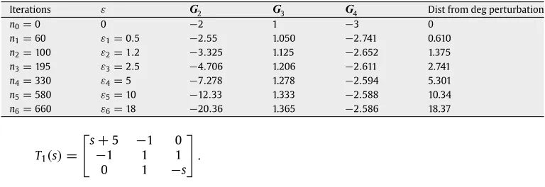
and so on.

Example 5.1.Consider a network whose system matrixT1

(

s

)

is defined by:

T1

(

s

)

=

⎡

⎣G1

+

₋

GG22

+

sC G2

−

+

G2G3 01

0 1

−

sL

−

(

1

/

G4

)

⎤ ⎦

when the values are: C

=

1,L

=

1,G1

=

4,G2

=

1,G3

=

0,G4

= ∞

, then the system matrix

[image:14.468.38.422.88.220.2]

Table 1

Summary of the Quasi-Newton computations Algorithm for Example (5.1).

Iterations ε G₂ G₃ G₄ Dist from deg perturbation

n0=0 0 −2 1 −3 0

n1=60 ε1=0.5 −2.55 1.050 −2.741 0.610 n2=100 ε2=1.2 −3.325 1.125 −2.652 1.375 n3=195 ε3=2.5 −4.706 1.206 −2.611 2.741 n4=330 ε4=5 −7.278 1.278 −2.594 5.301 n5=580 ε5=10 −12.33 1.333 −2.588 10.34 n6=660 ε6=18 −20.36 1.365 −2.586 18.37

T1

(

s

)

=

⎡

⎣s

₋

+

15

−

11 01

0 1

−

s

⎤ ⎦

_.

Assuming that we would like to change the natural frequencies of the above system by tuning the values ofG2,G3,G4, we define the following perturbation:

⎡

⎣

₋

GG22 G2

−

+

G2G3 00

0 0 G4

⎤ ⎦

₌

⎡

⎣

₋

11 01 00

0 0 1

⎤ ⎦ ⎡

⎣G02 G03 00

0 0 G4

⎤ ⎦ ⎡

⎣10

−

11 00

0 0 1

⎤

⎦

₌

UΛUt,

which is equivalent to applying a diagonal perturbationΛ

=

diag

(

G2,G3,G4

)

to the modified system

U−1T1

(

s

)(

Ut

)

−1

=

⎡

⎣ss

+

+

54 ss

+

+

44 01

0 1

−

s

⎤ ⎦

The equations defining the degenerate perturbations are:

f2

(

G2,G3,G4

)

= −

1

−

G2

−

G3

=

0

f1

(

G2,G3,G4

)

= −

5

−

4G2

−

5G3

−

G2G3

+

G4

+

G2G4

+

G3G4

=

0

f0

(

G2,G3,G4

)

= −

5

−

G2

+

4G4

+

4G2G4

+

5G3G4

+

G2G3G4

=

0

and the finite solutions of these equations are given by:

(

a

)

G2

= −

2,G3

=

1,G4

= −

3

;

(

b

)

G2

=

0,G3

= −

1,G4

= −

5

.

Note that both of the above solutions are full (regular) solutions, and thus both can be used as staring points for a numerical Quasi-Newton method to place the characteristic polynomial at any given second order one,

φ(

s

)

using the iterative procedure [21]:

x_n+1

=

x_n

−

(

JF

)

−_x1

0

(

f

−

ε

k

φ)

,

wherex

=

(

G2,G3,G4

)

t,

φ

= [

1, 8, 15

]

t,f

= [

f2,f1,f0

]

tandx0

=

(

−

2, 1,

−

3

)

t. Starting with a value

ε

1

=

0

.

5, the method converges after about 60 iterations tox60

=

(

−

2, 5507, 1, 050697,

−

2, 74137

)

t.

Taking now this as a starting point we repeat the method for

ε

2

=

1

.

2 and so on. Table 1 displays the

various solutions we obtain through this algorithm the last column being the Euclidean distance of the solution from the degenerate one. The final row refers to the solutionG2

= −

20, 36,G3

=

1, 365,G4

=

−

2, 586 which is the furthest away from the degenerate compensator. This compensator is achieved after 660 iterations, it assigns the zeros

−

2, 99915 and

−

4, 99982 (

−

3 and

−

5 were the required ones) and its distance from the degenerate compensator is 18, 37.

6. Necessary and sufficient condition for arbitrary assignment in the complex domain: the case rank

(

A

)

=

n

(

A

)

=

n, there are no degenerate compensators and the above approach cannot be deployed. In this case we will follow the approach in [15], which is based on the examination of the rank properties of the differential of the mapF. In fact, the rank of the differential of a complex algebraic map, although it is a local invariant, it may determine global properties of this map. The following lemma explains how this rank is related with the (almost) surjectivity property ofF. Note that by “almost onto” it is meant that all polynomials, but a negligible set can be assigned.

Lemma 6.1(Dominant Morphism[14,15]).If F is an algebraic map between two complex varieties X,Y for whichdimXdimY,then there exists x in X such thatrankDFX

=

dimY,iff F is

(

almost

)

onto

.

This shows that the invariant that characterizes the onto property of the mapFis thenth exterior product of its differentialDFX. In the case we examine, this invariant is the determinant of the Jacobian

ofF, i.e. det

(

J

(

F

)

X

)

. AsFcan be factored as [15]:

F

:

C

n T

→

C

σ

→

P

C

n, (6.1)

where

T

(

x

)

=

n

i=1

(

1,xi

)

, F

(

x

)

=

T

(

x

)

·

P and

σ

=

2n (6.2)

the Jacobian of the zero assignment map can be calculated in terms of the Jacobian ofTand the Plucker matrixP[18]. By the Binet Cauchy theorem det

(

J

(

F

))

can be factored as a product of two compounds as follows:

det

(

J

(

F

)

x

)

=

Cn

(

J

(

T

))

·

Cn

(

P

).

(6.3)

The compoundCn

(

P

)

is a vector containing the system parameters, whereas the vectorCn

(

J

(

T

))

con-tains the structure implied by the diagonal structure of the controller. The calculation of det

(

J

(

F

)

x

)

is

thus reduced to calculatingCn

(

J

(

T

))

. The calculation ofJ

(

T

)

can be easily performed as shown by the

following lemma:

Lemma 6.2[15].The partial derivative of T with respect to xi,is given by

:

∂

T

/∂

xi

= ⊗

(

1,x1

)

⊗ · · · ⊗

(

1,xI−1

)

⊗

(

0, 1

)

⊗

(

1,xI+1

)

⊗ · · · ⊗

(

1,xn

).

(6.4)

Selectnentries of the vectorT

(

x

)

saya

= [

al,a2,

. . .

,an

]

, and call the Jacobian of the functiona,J

(

a

)

;

then this is a squaren

×

nmatrix whose determinant is one of the coordinates of the vectorCn

(

J

(

T

))

;

conversely, all the coordinatesCn

(

J

(

T

))

are of the form det

(

J

(

a

))

for somea, i.e. Cn

(

J

(

T

))

=

(

det

(

J

(

a

))

a

.

The following result is central in providing an expression for the JacobianJ

(

a

)

needed for the description for the compoundCn

(

J

(

T

))

.

Proposition 6.1[15].The Jacobian J

(

a

)

is given by

:

J

(

a

)

=

diag

x−_l 1,x−₂1,

. . .

,x−_n1

I

(

a

)

diag

(

al,a2,

. . .

,an

)

, (6.5)

where the ij entry of I

(

a

)

is 1 if ajcontains the xiand it is 0 otherwise

.

Therefore the determinant of J

(

a

)

is expressed as

:

det

(

J

(

a

))

=

I

(

a

)

a1,a2

. . .

an

/

x1x2

· · ·

xn

.

(6.6)

From the above we have the following description ofCn

(

J

(

T

))

.