High Speed Inverse Model Implementation for Real-Time
Control of Distributed Parameter Systems Operating
in Nonlinear and Hysteretic Regimes
Thomas R. Braun and Ralph C. Smith
Abstract— Ferroelectric (e.g., PZT), ferromagnetic, and fer-roelastic (e.g., shape memory alloy) materials exhibit varying degrees of hysteresis and constitutive nonlinearities at all drive levels due to their inherent domain structure. At low drive levels, these nonlinear effects can be mitigated through feedback mechanisms or certain amplifier architectures (e.g., charge or current control for PZT) so that linear models and control designs provide sufficient accuracy. However, at the moderate to high drive levels where actuators and sensors utilizing these compounds often prove advantageous, hysteresis and constitutive nonlinearities must be incorporated into models and control designs to achieve high accuracy, high speed control specifications. In this paper, we employ a homogenized energy framework to characterize hysteresis in this combined class of ferroic compounds. We then use this framework to construct highly efficient inverse models that can be used to approximately linearize actuator dynamics for subsequent linear control design. For applications such as high speed tracking (e.g., kHz rates) or broadband vibration attenuation, the efficiency of the inverse construction proves crucial for real-time control implementation. We demonstrate aspects of the inverse model implementation in the context of rod models used to characterize PZT and magnetic actuators presently employed in applications ranging from nanopositioning to high speed milling of automotive components.
I. FERROELECTRIC ANDFERROMAGNETIC
TRANSDUCERS
Ferroelectric and ferromagnetic materials are employed in a wide variety of applications as both actuators and sen-sors, including fluid pumps, nanopositioning stages, sonar, vibration control, ultrasonic sources, and high-speed milling. They are attractive because the transducers are solid-state and often very compact. However, the coupling of nonmechanical field to mechanical deformation, which makes these materials effective transducers, also introduces hysteresis and time-dependent behavior that must be accommodated by con-trollers. Classically, this has been attained by operating the transducer in only a small portion of its theoretical operating range and/or operating it at a low frequency. This allows controllers to accommodate nonlinear dynamics but reduces
Supported by the US Department of Education GAANN Fellowship and the Air Force Office of Scientific Research under grant AFOSR-FA9550-04-1-0203.
Thomas R. Braun is with the Center for Research in Scientific Computing, Department of Mathematics, North Carolina State University, Raleigh NC, 27606 USA (email:[email protected])
Ralph C. Smith is with the Center for Research in Scientific Computing, Department of Mathematics, North Carolina State University, Raleigh NC, 27606 USA (email:[email protected])
the performance of the transducer. More sophisticated ap-proaches incorporate these dynamics through electromechan-ical or magnetomechanelectromechan-ical models. In theory, this permits high-speed, high-accuracy control, but in practice introduces significant computational overhead which limits effective-ness. If the reference trajectory is known a-priori, a nonlinear control may be utilized which allows the computation to be performed a-priori as well (see [6]). Alternatively, one can employ a model-based inverse compensator to form a composite system which is approximately linear and time-invariant. We focus on this latter approach and construct highly efficient implementation algorithms.
II. DEVICEMODEL
Several different models exist for ferroelectric and fer-romagnetic materials. These include domain wall models, Preisach models, and homogenized energy models. Infor-mation and numerous references for these models may be found in [7]. We employ the homogenized energy model due to its solid basis in the underlying physics of the material, its ability to characterize effects such as minor loops and creep in a natural manner, and its applicability to both ferroelectric and ferromagnetic materials. Since we are typically interested in controlling the displacement and not the polarization or magnetization, the dynamics of the actuator, including its interface in with various plants, must also be incorporated. This is illustrated for the case when the actuator is a rod.
A. Homogenized Energy Model Development
The homogenized energy model for ferroelectric materials is
P(E;x+) =
Z ∞
0
Z ∞
−∞
νc(Ec)νI(EI)
·P(E+EI;Ec;x+)dEIdEc
(1)
1) bothνc andνI are bounded by decaying exponentials, 2) νc is strictly positive,
3) νI is symmetric about 0, and 4) R0∞νc(Ec)dEc= 1, R∞
−∞νI(EI)dEI = 1.
The integrals are solved numerically via quadrature, i.e.,
P(E;x+) = Nc
X
i=1
NI
X
j=1
νc(Ec[i])νI(EI[j])wc[i]wI[j]
·P(E+EI[j];Ec[i];x+[i, j])
(2)
wherewc andwI give the quadrature weights. As detailed in [7], the model for magnetic materials is equivalent. There-fore, to simplify discussion, we formulate equations solely in terms of the electric field and polarization, with the un-derstanding that everything applies equally to ferromagnetic materials.
The kernel P is modeled through energy principles. The mesoscopic Helmholtz energy is taken to be
ψ(P) =
η(P+PR)2/2, P ≤ −P
I
η
2(PI−PR)
P2 PI
−PR
, |P|< PI
η(P−PR)2/2, P ≥PI
(3)
wherePI denotes the positive inflection point at which the switch occurs, PR is the local remanence polarization, and
η is the reciprocal slope ∂E∂P. The Gibb’s free energy
G=ψ−EP (4)
balances this internal Helmholtz energy with the electrostatic energy; i.e., work performed by the applied external field. This energy must be balanced with the thermal energy of the material through Boltzmann’s relation. As shown in [7], [8], [10], the resulting kernel is
P =x+hP+i+ (1−x+)hP−i (5)
wherex+∈[0,1]denotes the fraction of positively oriented dipoles and
hP+i=
R∞
PI Pexp
−G(E+EI,P)V
kT
dP
R∞
PIexp
−G(E+EI,P)V
kT
dP ,
hP−i=
R−PI
−∞ Pexp
−G(E+EI,P)V
kT
dP
R−PI
−∞ exp
−G(E+EI,P)V
kT
dP
(6)
are the average polarizations associated with positive and negative dipole orientations. Here V is the volume of the mesoscopic layer modeled by the kernel,k is Boltzmann’s constant, andT is the temperature. The evolution of dipole fractions is governed by the differential equation
˙
x+=−p+−x++p−+(1−x+), (7)
where the likelihoods p+− and p−+ of a dipole switching from positive to negative, or vice-versa, are
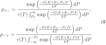
p+−=
exp
−G(E+EI,PI)V
kT
dP
τ(T)R∞
PI exp
−G(E+EI,P)V
kT
dP,
p−+=
exp
−G(E+EI,−PI)V
kT
dP
τ(T)R−PI
−∞ exp
−G(E+EI,P)V
kT
dP
(8)
and τ quantifies the material and temperature-dependent relaxation time. Note that the local coercive fieldEc, local remanence polarization PR, and inflection point PI are related by the expression
PI =PR−
Ec
η . (9)
B. Displacement Model
As detailed in [7], both nanopositioning stages employed in common atomic force microscope designs and magnetic transducers employed for high speed milling utilize ferro-electric and ferromagnetic rods that are clamped at one end and subject to damped restoring forces at the other. Hence we consider a rod of length ℓ and cross sectional area A
as depicted in Figure 1. The end mass mℓ with damping
cℓ and stiffness kℓ encompass adjacent transducer and plant dynamics.
It is shown in [7], the constitutive relation for the induced stress is given by
σ=Y ε+Cε˙−a1(P−P0)−a2(P−P0)2 (10)
where Y is the Young’s modulus of the transducer, C is the Kelvin-Voight damping coefficient, P0 is the point the material is poled around, a1 and a2 are constants of pro-portionality relating the induced polarization to mechanical force, andP =P(E;x+)is given in (2).
Due to the distributed nature of the device, partial dif-ferential equation models have been developed in [7], [9] to characterize the device dynamics. However, for a number of motivating applications, it has been shown that because forces and fields are uniform in space, strains and hence displacements are also uniform thus permitting the use of ordinary differential equation representations. In this case, the strain is given by
ε= uℓ
ℓ (11)
x=0 x=l
u
k
c
l
ml
l
Fig. 1. Rod used to construct the system model. The end massmℓ, stiffness
where uℓ(t) = u(t, ℓ) denotes the displacement of the rod tip.
By balancing forces we obtain
md 2u
ℓ
dt2 +c duℓ
dt +kuℓ=α1(P−P0) +α2(P−P0) 2 (12)
whereρis the density of the rod and
m=ρAℓ+mℓ, c=
CA
ℓ +cℓ, k= Y A
ℓ +kℓ, α1=Aa1, α2=Aa2.
Further details may be found in [7], [9].
C. Efficient Implementation Formulation
The coupled polarization and rod models can be simplified to increase their computational efficiently. For the homoge-nized energy model, it is shown in [1] that the polarization can be expressed as
P(E;x+) =E
η −PR+
Nc X i=1 NI X j=1
wc[i]wI[j] x+ pos
+neg+k1−neg
(13)
where
wc[i] =
s
2kT
πV ηνc(Ec[i])wc[i],
wI[j] =νI(EI[j])wI[j], k1=PR
r
2πV η kT .
pos= exp
− V
2kT η(−E−EI−Ec)
2
erfc
q
V
2kT η(−E−EI−Ec)
,
neg= exp
−2kT ηV (E+EI−Ec)
2
erfc
q
V
2kT η(E+EI−Ec)
.
The evolution of moment fractions can be approximated by a backward Euler discretization; thus
x+(t+ ∆t) = k2
∆tx+(t) +neg k2
∆t+neg+pos
(14)
where
k2=τ(T)
s
πkT
2V η.
Similar approaches can be taken with the rod model. In this case, we will assume P does not change between timesteps which permits us to solve (12) analytically. As-suming the step-size∆tis fixed, the rod model then becomes
u(t+ ∆t) =d1u(t) +d2u˙(t) +m
k (1−d1)v(t+ ∆t),
˙
u(t+ ∆t) =d3u(t) +d4u˙(t) +−d4m
k v(t+ ∆t).
(15) where
v=α1(P−P0) +α2(P−P0)2
and the constants d1, . . . , d4 depend on the the parameters
m,c, andk. Let ˜c=c/mand˜k=k/m. If˜c2>4˜kthen
d1= 1 2
1−˜c
z
exp
−1
2(˜c+z) ∆t
+
1 + ˜c
z
exp
−1
2(˜c−z) ∆t
,
d2= 1
z
exp
−1
2(˜c−z) ∆t
−exp
−1
2(˜c+z) ∆t
,
d3= 1 4
˜
c2
z −z exp
−1
2(˜c+z) ∆t
−exp
−1
2(˜c−z) ∆t
,
d4= 1 2
1 + ˜c
z
exp
−1
2(˜c+z) ∆t
+
1− ˜c
z
exp
−1
2(˜c−z) ∆t
,
(16)
wherez=p˜c−4˜k. Analogous expressions can be obtained for the cases˜c2= 4˜k and˜c2<4˜k, see [1].
As detailed in [1], the primary computation time required to implement the discretized rod model (15) is required for computation of P via the homogenized energy model (2). This is specifically dictated by the number of quadrature points and the computation ofposandnegat each quadrature point. Utilizing lookup table or polynomial approximations (see [1]) and 40 quadrature points for each distribution (1600 total), the rod model can be run at well over 10,000 timesteps per second on a modern desktop or laptop computer. At 10 samples per cycle, this is equivalent to an operating frequency of 1 kHz. If 20 quadrature points per distribution (400 total) are sufficient for the application in question, this increases to over 40,000 timesteps per second or 4 kHz.
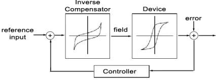
III. INVERSEFILTERCONSTRUCTION
As discussed in Section I, one method to accurately control a smart material actuator involves the use of an inverse compensator or filter. A prototypical setup for this type of control is depicted in Figure 2. The material is non-linear, hysteretic, and time-varying, but these attributes are approximately linearized by the inverse filter. The composite system to be controlled is then approximately linear and time-invariant. This allows simple control designs including PI/PID and LQR designs to be utilized.
The inverse compensator is simply the inverse of our model. Inverting the rod equation is straightforward. Assum-ing∆tis fixed, inverting (15) gives
v(t+ ∆t) = 1
d3bu(t+ ∆t)− d1 d3bu(t)−
d2
d3bu˙(t) (17)
whereu(t) is now the desired displacement value. Once v
Fig. 2. Depiction of an actuator control utilizing an inverse filter coupled with a linear control law.
determined from the quadratic formula, namely
b
P(t) =P0− α1 2α2 ±
s
α1
2α2
2
+mv(t)
a2 (18)
as long asα26= 0. Ifα2 is 0, the equation is linear and the solution is
b
P(t) =P0+ m
α1v(t). (19)
Note that forα26= 0 either polarization value is acceptable, as both give equivalent displacements. However, to minimize the effects of modeling error, a single branch should always be utilized.
Once the desired polarization P is determined, the ho-mogenized energy model can be inverted to determine the required field. Such an inversion cannot be done analytically, however. Instead at each timestep we formulate the inverse model as a root-finding problem, namely determining the value ofE such that
P(E;x+)−Pb= 0. (20)
Here,P(E;x+)is the homogenized energy model (2). The state x+ can be maintained as the model runs, and for a given timestep it is thus a known, fixed quantity.
The structure of (20) introduces both simplification and difficulties into the root-finding problem. First, sincex+is a fixed, known value for a given timestep (changing between timesteps, but not during each root-finding problem itself), (20) is monotone increasing inE. However, a consequence of the the quadrature in (2) is that (20) contains regions where the slope is very steep. It is not feasible to resolve these re-gions numerically. This yields an equation that is effectively discontinuous; the large slope regions appear numerically as a finite number of simple jumps. It can be shown that the height of these jumps depends on the relaxation amount
V /kT, with the height decreasing as V /kT → 0, and that the height is also proportional to the number of quadrature points, more specifically to νc(Ec[i])νI(EI[j])wc[i]wI[j]. However, increasing the number of quadrature points in-creases the computation required, so we must accept that the equation may contain some discontinuities and handle these discontinuities in the root-finding problem.
A. Discontinuous Root Finding
If (20) was continuously differentiable, the secant method would provide nearly optimal convergence to the solution in terms of function evaluations[4]. However, for a discon-tinuous function it may not converge. The bisection method will converge, but often this convergence is slow. Methods exist which combine bisection with interpolation to attempt to improve this rate; see [2] for example. However, we saw better performance by exploiting the monotone nature of the function to directly improve the convergence of the bisection method.
The bisection method, or any other method which utilizes it, requires both that the root be bounded and that the function change signs within the bounds. For a monotone function, these requirements are the same. Theoretical bounds on E
may be computed by considering the case when all dipoles have switched. In these cases (all dipoles positive or all negative), E can be determined analytically. The required value of E is by necessity between these extreme cases, namely
η(Pb−PR)≤E ≤η(Pb+PR). (21) However, directly applying bisection with these bounds yields slow convergence, because the bounds are large.
Instead, we turn to the secant method as a way to calculate tighter bounds. The secant method does not require bounds, but instead uses approximate derivatives to converge to the root. Since the function is not smooth, this may not converge. However, the monotone nature of the function dictates secant will always step in the correct direction. Thus, on each iteration either the secant method does not step far enough, in which case the function value is reduced in magnitude, or the method steps too far. In this latter case the function value may be reduced or increased in magnitude, but either way the iterations have crossed over the root value. Thus, each iteration of the secant method will either provide a better approximate for E or provide a bound on the root. We therefore apply the secant method to (20) first. If there is sufficient relaxation or the valuePb does not lie near any discontinuities, we obtain rapid convergence. If the secant method fails to converge, the secant iterations themselves are utilized to determine the bound on the root, which can then be given to bisection to find the actual root. These bounds are typically much tighter than (21), which improves the convergence of the bisection method. For the purposes of our algorithm, failure to converge in the secant method is defined as
|P(Ei;x+)−Pb| ≥ |P(Ei−2;x+)−Pb|, for alli≥3 (22)
whereEiis the value ofEdetermined by the ith iteration of the secant method. Such a definition is a heuristic to detect failure quickly without penalizing a single poor step.
using the previous two time steps of the model, in a manner analogous to how the secant method itself approximates derivatives. This approximation is simply ∆P/∆E, where ∆P is the difference inP(E;x+)for the previous two time steps, and ∆E is the corresponding differences in E. The latter approximation is deemed more accurate, and is utilized when the previous two time steps are known. When this is not the case, 1/η is utilized as the initial derivative. The computed derivative value should also be checked against this lower limit on each iteration of the secant method, to trap some errors that may arise with the subtraction of nearly equal numbers.
B. Inverse Model Validation
The accuracy and performance of the inverse rod and homogenized energy models can be observed by computing the electric or magnetic field needed to achieve a specified reference displacement, and then inputting this field to the homogenized energy model to determine the predicted dis-placement. The absolute difference between reference and predicted displacements gives the error, which is a combina-tion of error in the numerical root-finding and the error in inherent in the homogenized energy model due to quadrature induced “discontinuities”. Such a comparison is computed in Figure 3 for parameters obtained for a Terfenol-D rod. Note that whereas the displacement is specified in microns, the error is in picometers. A very tight tolerance was utilized in the figure, so that the observed error is primarily modeling error introduced by quadrature. The number of calculation of the forward model needed for various tolerances in the numerical root-finding (for the example input in Figure 3) is given in Table I. We see for this input and parameter set that about 6.5 evaluations are needed on average, and 19 in the worst-case, to achieve a positioning accuracy of 10 nm, which is over three order of magnitude below the size of the stroke. These results are typical, although different inputs and material parameters would give slightly different results.
IV. PI CONTROL
Figure 3 and Table I illustrate that the inverse compensator approach effectively provides an accurate open-loop control as long as the model accurately describes the transducer. In cases where modeling error must be considered, a feedback controller may be utilized as depicted in Figure 2. To
Error Average Maximum
tolerance model evaluations model evaluations
1 micron 2.1240 8
100 nm 2.2880 9
10 nm 6.5170 19
1 nm 11.6500 22
100 pm 14.7040 25
10 pm 17.6930 29
TABLE I
EFFORT TO COMPUTE THE INVERSE MODEL IN TERMS OF AVERAGE AND
MAXIMUM NUMBER OF FUNCTION EVALUATIONS.
0 0.02 0.04 0.06 0.08 0.1 −20
−10 0 10 20 30 40 50
Time (s)
Displacement (microns)
(a)
0 0.02 0.04 0.06 0.08 0.1 −2
−1 0 1 2 3 4 5
Time (s)
Magnetic Field (kA/m)
(b)
0 0.02 0.04 0.06 0.08 0.1 0
2 4 6 8 10 12 14 16 18
Time (s)
Displacement Error (pm)
(c)
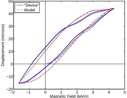
illustrate this, we take two different sets of parameters to the homogenized energy and rod models, one to give the model while the other simulates a physical device. The parameters are chosen to include some modeling error, as shown in Figure 4. The positioning error of an open-loop control using this model for the device is shown in Figure 5. As can be seen, the peak error is about 7.5 microns and the RMS error is roughly 3.8 microns. No noise was added to this example. This is fairly accurate for an open loop control, and the accuracy level is driven by the difference between the device and the model. However, better results can be obtained. If a PI feedback is introduced to the composite system depicted in Figure 3, the result is twice as good in terms of peak error, over 7 times better in RMS error. This is illustrated in Figure 5 as well forkp= 0.35andkI = 11,000. Peak and RMS errors for various noise levels with the PI control are given in Table II.
More sophisticated controls are certainly possible, and better model fits are often obtainable as well. The simple
−2 −1 0 1 2 3 4 5
−20 −10 0 10 20 30 40 50
Magnetic Field (kA/m)
Displacement (microns)
"Device" Model
Fig. 4. Model and “Device” behavior for the control examples given in Section IV.
0 0.02 0.04 0.06 0.08 0.1 −4
−2 0 2 4 6 8
Error (microns)
Time(s)
Open loop PI control
Fig. 5. Comparison of open-loop and PI controls utilizing the inverse compensator for the model and “device” given in Figure 4.
Noise standard deviation Peak error RMS error
0 3.14 0.517
0.1 3.10 0.527
0.5 5.07 0.863
1.0 6.06 1.45
TABLE II
ERROR FOR VARIOUS LEVELS OFGAUSSIAN NOISE FOR THEPI
CONTROL WITH THE INVERSE COMPENSATOR,UTILIZING THE DEVICE
AND MODEL DEPICTED INFIGURE4. ALL UNITS ARE IN MICRONS.
control and mediocre model fit are chosen intentionally to illustrate the accuracy of the inverse compensator even when dealing with noise and modeling error.
V. CONCLUDINGREMARKS
We have shown that the inverse compensator provides an efficient and accurate method to determine the field value needed to control an actuator to a desired displacement. This allows a linear, time-invariant control to be employed to a nonlinear, hysteretic, and time-varying transducer, even in cases where the modeling error is moderate. Since the only significant source of computational effort is the inverse ho-mogenized energy model, this control is capable of running in about 15 to 101 of the speed of the forward homogenized energy model on average, or about 201 of the speed in the worst-case scenario. Designing to the worst case, we obtain a system capable of roughly 500 - 2000 timesteps per second on conventional desktop or laptop computers (or assuming 10 timesteps per cycle, at speeds up to 200 Hz). This provides the full dynamic range of the actuator and does not require
a-priori knowledge of the system.
REFERENCES
[1] T.R. Braun and R.C. Smith, “Efficient inverse compensation for hysteresis via homogenized energy models,” preprint.
[2] R.P. Brent, Algorithms for Minimization without Derivatives, Prentice-Hall, Englewood Cliffs, N.J., 1973.
[3] A.G. Hatch, R.C. Smith, T. De, and M.V. Salapaka, “Construction and experimental implementation of a model-based inverse filter to attenuate hysteresis in ferroelectric transducers,” IEEE Transactions
on Control Systems Technology, 14(6), pp. 1058-1069, 2006.
[4] C.T. Kelley, Iterative Methods for Linear and Nonlinear Equations, SIAM, Philadelphia, 1995.
[5] W.H. Press, S.A. Teukolsky, W.T. Vetterline, B.P. Flanner, Numerical
Recipes in C, Second Edition, Cambridge University Press, New York,
1992.
[6] W.S. Oates, P. Evans, R.C. Smith, and M.J. Dapino, “Experimental implementation of a nonlinear control method for magnetostrictive transducers,” Proceedings of the 46th IEEE conference on Decision and Control, 2006.
[7] R.C. Smith, Smart Material Systems: Model Development, SIAM, Philadelphia, 2005.
[8] R.C. Smith, M.J. Dapino, T.R. Braun and A.P. Mortensen, “A ho-mogenized energy framework for ferromagnetic hysteresis” IEEE
Transactions on Magnetics, 42(7), pp. 1474-1769, 2006.
[9] R.C. Smith, A.G. Hatch, T. De, M.V. Salapaka, R.C.H. del Rosario, and J.K. Raye,“Model development for atomic force microscope stage mechanisms,” SIAM Journal on Applied Mathematics, 66(6), pp. 1998-2026, 2006.
[10] R.C. Smith, S. Seelecke, Z. Ounaies and J. Smith, “A free energy model for hysteresis in ferroelectric materials,” Journal of Intelligent