A continuous stochastic disaggregation model of rainfall for peak flow simulation in urban hydrologic systems

A Continuous Stochastic Disaggregation Model of Rainfall for Peak

Flow Simulation in Urban Hydrologic Systems

Paul S.P. Cowpertwait

I.I.M.S., Massey University Albany Campus, Auckland, New Zealand

[email protected]

Abstract

In the paper by Durrans et al. (1999), an algorithm proposed by Ormsbee (1989) is recommended for the stochastic disaggregation of hourly rainfall in continuous flow simulation studies of urban hydrologic systems. However, Durrans et al. found that the method produced a “severe negative bias” in the maximum rainfall intensity of the disaggregated series, so that peak flows in urban systems are likely to be under-estimated by the model. Here we develop a method for disaggregating hourly data to 5min series, which addresses the problem of negative bias. A regression equation is derived for the ratio of the maximum 5min depth to the total depth in the hour. Thus, for any given hourly depth this ratio can be simulated and multiplied by the hourly depth to obtain a 5min maximum. The temporal location of the maximum within the hour can be randomly placed using an appropriate distribution function, e.g. based on a geometrical construction as developed by Ormsbee (1989). The model is developed and tested using 5min rainfall data taken from Lund (1923-39) and Torsgatan (1984-93), Sweden. The results support the use of the model in urban drainage applications.

Introduction

As part of a UK Urban Pollution Management Programme, initiated by the Water Research Centre (e.g. see Tyson and Clifforde 1989, or Crabtree 1988), Cowpertwait et al. (1996a,b) developed a regionalised stochastic rainfall generator. This generator incorporates a Neyman-Scott point process model for the simulation of hourly rainfall (e.g. see Cowpertwait, 1998), and an algorithm proposed by Ormsbee (1989) for stochastically disaggregating the generated hourly data into 5min values. The generator has been further developed for use in Sweden as part of a European Union Technology Validation Project (Threlfall et al., 1998, 1999). In this paper, we present results from that project which help address the problem of negative bias in the maximum intensities of the disaggregated rainfall, recently reported by Durrans et al. (1999).

The proposed method uses a regression model to predict the ratio of the maximum 5min depth to the hourly depth, thus enabling a 5min maximum to be simulated for any given hourly depth. The distribution function proposed by Ormsbee (1989) can be used to assign the maximum to a 5min interval within the hour. The model is appropriate for problems in urban wastewater management, as it is likely to give representative peak flows in hydrologic models of sewer networks (Threlfall et al., 1998, 1999). The same methodology could be applied to disaggregate hourly data to intervals smaller or larger than 5 minutes (e.g. one-minute series or 15-minute series).

Data

Formulation of regression model

An appropriate regression model for the ratio Y should contain information known about Y (e.g. 0 ≤ Y ≤ 1) and include possible explanatory variables (e.g. seasonal indicator variables). We thus proposed the following model:

1 11 1 0

exp

1

ïþ

ï

ý

ü

ïî

ï

í

ì

÷÷

ø

ö

çç

è

æ

₊

₊

+

=

å

j ij j

i

c

c

I

Z

Y

where Yi is the ith ratio (i = 1, …, 2269), cj are regression coefficients (j = 0, 1, …, 11), and Zi is the ith

residual error. The Iij are indicator variables taking the values: Iij = 1, when the ith ratio is in the jth

season, or Iij = 0, otherwise. Note that the model has 12 seasons corresponding to each calendar month

(with ‘1’ corresponding to January, ‘2’ to February, etc); with only eleven indicator variables being needed because of the constant term c0.

In order to estimate the coefficients cj, the ratio Y was transformed using a logit transformation to

give the predictor variable Y ′ given by:

(

)

j ij j i

i

Y

c

c

I

Z

Y

′

=

−

=

+

å

+

= − 11 1 0 1

₁

ln

The estimation of the coefficients cj therefore reduces to fitting a linear regression model which is

achieved by least squares estimation. Note that E(Zi) = 0, so that predicted values of Y ′ will be unbiased.

Conversely, the predicted values of Y will be biased because of the transformation

_Y

=

(

1

+

_e

)

However, this is of no concern here because we will simulate values of Y, which will be unbiased under the transformation.

The least squares estimates of the coefficients cj are shown in Table 1, where it can be seen that

there is a slight difference in the predicted ratios for summer and winter, with summer months tending to have higher predicted ratios and, therefore, more high-intensity 5min rainfalls. This reflects the well-known meteorological observation that more frequent high-intensity convective storms occur during summer months, with more low-intensity frontal storms occurring in winter.

Table 1

Fitted regression coefficients and statistical tests*

Coefficient Estimate SD T P

C0 1.96 0.520 3.77 0.000

C4 -0.995 0.735 -1.35 0.178

C5 -1.16 0.559 -2.07 0.039

C6 -1.20 0.539 -2.23 0.026

C7 -1.04 0.526 -1.97 0.050

C8 -0.945 0.528 -1.79 0.075

C9 -0.784 0.532 -1.47 0.142

σz = 0.735

* Coefficients not listed are estimated as zero

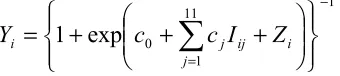
From Table 1, the equation for simulating a ratio of the maximum 5min depth to the hourly depth is given by:

Y = {1 + exp(2.0 – 1.0 I4 - 1.2 I5 - 1.2 I6 - 1.0 I7 - 0.95 I8 - 0.78 I9 - 0.62 I10 + Z)}-1

(3) where Z is a simulated Normal random variable with mean zero and standard deviation 0.735 (the subscript i has been omitted without loss of generality). The fitted regression model (3) only explained about 6% of the variation in the data, so that a reasonable approximation can be obtained by neglecting the seasonal indicator variables, i.e. using the model:

Y = {1 + eZ_}-1 ₍₄₎

where Z is approximately Normally distributed with mean 1.3 and standard deviation 0.77.

An analysis of the residual errors in the fitted model (2) revealed a slight departure from the Normal distribution in the far tail of the probability plot (Figure 1). This may result in some under-estimation of the very extreme 5min intensities when using the Normal distribution. A possible alternative would be to use the empirical distribution of the residuals in simulation, but this would clearly restrict the simulation to past historic values only.

3 2

1 0

-1 -2

-3 1

0

-1

-2

-3

Normal Score i

Normal Probability Plot of the Residuals

Resi

du

al

Figure 1: Probability plot for the residual errors in the fitted regression model

Inclusion of site indicator variables, to allow for different ratios at the two sites, had the effect of increasing the residual standard deviation (from 0.735 to 0.736), suggesting that the model can be applied without site indicator variables. This supports the argument that most of the variance in rainfall over a geographical region is explained by data sampled at time intervals greater than 5 minutes. Hence, it is reasonable to hypothesize the use of the same fitted disaggregation model at other urban sites not used in the fitting procedure.

Stochastic Disaggregation

Hourly rainfall can be disaggregated into 5min values using the fitted regression model with an appropriate probability distribution for assigning rain within the sub-hourly intervals. The steps below use the fitted model with the probability distribution function proposed by Ormsbee (1989).

(2) The simulated ratio is multiplying by the hourly rainfall depth x (mm) to obtain a simulated maximum 5min depth (xy). The remainder (1 – y)x will be distributed over the hour using pulses of depth 0.01mm, i.e. 100(1 - y)x pulses (see step 8 below).

(3) The probabilities mass function (p1, p2, …, p12) is found using an appropriate method, e.g. the

geometrical construction proposed by Ormsbee (1989), where pi is the probability that a depth (or

‘pulse’) of rain falls in the ith interval (i = 1, …, 12; p1 + p2 +…+ p12 = 1).

(4) The cumulative distribution function F(i) = p1 + p2 + … + pi is found for each 5min interval in the

hour (i = 1, …, 12, F(0) = 0, F(12) = 1).

(5) A uniform U(0,1) random number is generated to determine which interval to assign the maximum 5min depth. For example, if F(i-1) < U < F(i), the depth is assigned to the ith interval (i = 1, …, 12). (6) The probability mass function in step (3) is modified to ensure no pulses of rain fall in the same

interval as the maximum 5min depth. For example, if the maximum depth falls in the ith interval, the following re-assignments are made: pi+1→ pi+1 + ½ pi , pi-1→ pi-1 + ½ pi , after which pi→ 0 (i = 2,

3, …, 11). For i = 1, pi+1→ pi+1 + pi and pi→ 0. For i = 12, pi-1→ pi-1 + pi and pi→ 0.

(7) The cumulative distribution function F is modified using the modified probability mass function in (6) above.

(8) A uniform U(0,1) random number is generated and used with the distribution function F to determine which interval to assign a 0.01mm pulse of rain. This is repeated for each of the 100(1 - y)x pulses (from 3 above). Note that if 100(1 - y)x is a non-integer, then the decimal part d (mm) can be added to the first pulse to give a depth of 0.01+d (mm). In the unlikely event of an interval reaching the same level as the maximum, the probability for that interval can be assigned to zero and adjustments made to the probabilities for the adjacent intervals (as in 6 above).

(9) Steps (1) to (8) are repeated for each hour in the series to be disaggregated.

The above procedure ensures that the total hourly depth remains unchanged. In addition, Step 6 allows for some increase in intensity near the maximum in an attempt to preserve the autocorrelation expected in a 5min rainfall time series.

Tests on the model

To test the model, we selected two historical events from the Lund data: (i) the event having the largest total volume of rain (the ‘heaviest event’), and (ii) the event having the highest hourly intensity. Each of these events were aggregated to hourly time series and then disaggregated using the steps above.

For each event, time-series plots of the historical and disaggregated series were found and are given in Figures 2 and 3, where it can be seen that the disaggregation algorithm generates storm profiles which have a realistic appearance, representative of the historical events.

0.00 0.20 0.40 0.60 0.80 1.00 1.20 1.40

5 10 15

Time / hours

de

pt

h /

m

m

0 0.2 0.4 0.6 0.8 1 1.2 1.4

5 10 15

Time / hours

depth /

mm

Figure 2b: Time-series plot of the heaviest event when disaggregated

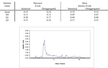
To provide more quantitative tests, sample statistics were evaluated for the historical and disaggregated series. These included the mean, standard deviation (SD), lower quartile (Q1), and upper quartile (Q3). In addition, the sample autocorrelation for a range of lags (the ‘correlogram’) was also found for each event.

Table 2 gives the sample statistics, where it can be seen that a reasonable fit is obtained to the historical values. In particular, the historical standard deviations are well matched by the simulated data even though they have not been used in the fitting procedure. A very slight under-estimation (of 0.05mm) in the distribution tail (Q3) is evident for the most intense event, but this is not likely to be of practical importance.

Table 2: Sample Statistics taken from Historical and Disaggregated Series

Heaviest Event

Most Intense Event Statistic

(mm)

historical Disaggregated historical Disaggregated

mean 0.25 0.24 0.32 0.32

SD 0.11 0.13 0.49 0.47

Q1 0.20 0.17 0.04 0.06

Q3 0.33 0.34 0.37 0.32

0.00 0.50 1.00 1.50 2.00 2.50 3.00 3.50 4.00 4.50 5.00

5 10

time / hours

de

pt

h /

mm

0 0.5 1 1.5 2 2.5 3 3.5 4 4.5 5

5 10

time / hours

de

pt

h /

mm

Figure 3b: Time-series plot of the most intense event when disaggregated

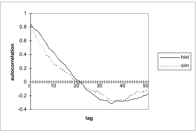
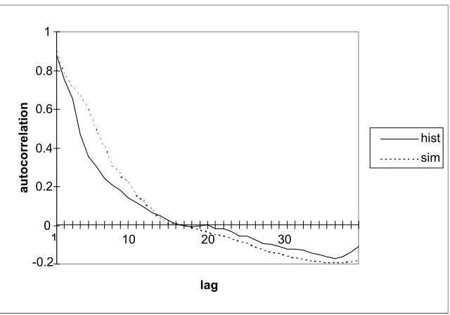
The correlograms (Figures 4 and 5) show a satisfactory representation of the correlation structure found in the historical events. For both events, the simulated and historical autocorrelations are approximately equal at lags 1 and reach zero at about the same lag. This is a very good result, particularly given that the disaggregation model does not use correlation in the fitting procedure, as in the case of traditional time-series models (e.g. ARIMA models).

-0.4 -0.2 0 0.2 0.4 0.6 0.8 1

1 10 20 30 40 50

lag

au

to

co

rr

el

at

io

n

hist sim

-0.2 0 0.2 0.4 0.6 0.8 1

1 10 20 30

lag

aut

o

correl

at

io

n

hist sim

Conclusions

The maximum rainfall intensity in a 5min interval can be simulated for a given hourly depth using the regression model described herein. The fitted regression model can be combined with the probability distribution function proposed by Ormsbee (1989) to disaggregate hourly rainfall into 5min values. This procedure corrects most of the negative bias in the maximum sub-hourly intensities, found when applying Ormsbee’s method.

Overall, the results support the use of the model for applications in urban hydrology and in the design and upgrading of sewer systems.

Acknowledgements

This research was produced as part of a Technology Validation Project IN101871 “Integrated Wastewater Project”, sponsored by the European Union Innovation Programme and coordinated by the UK Water Research Centre (WRc). Useful discussions with John Threlfall (WRc), Elliot Gill (WRc), and Håken Strandner (Danish Hydraulics Institute), are gratefully acknowledged.

References

Cowpertwait P.S.P., O’Connell P.E., Metcalfe A.V., J.A. Mawdsley, 1996a. Stochastic Point Process Modelling of Rainfall: I. Single-Site Fitting and Validation, J. Hydrology, 175, 17-46.

Cowpertwait P.S.P., O’Connell P.E., Metcalfe A.V. and J.A. Mawdsley, 1996b. Stochastic Point Process Modelling of Rainfall: II. Regionalisation and Disaggregation, J. Hydrology, 175, 47-65.

Cowpertwait P.S.P., 1998. A Poisson-cluster model of rainfall: high-order moments and extreme values, Proc. Royal Society, A, 454, 885-898.

Crabtree R., 1988. Urban River Pollution in the UK: the WRc River Basin Management Programme. In “Geomorphology in Environmental Planning”, edited by J.M. Hooke, John Wiley & Sons. Durrans S.R., Burian S.J., Nix S.J., Hajji A., Pitt R.E., Fan C., and R. Field, 1999. Polynomial-Based

Disaggregation of Hourly Rainfall for Continuous Hydrologic Simulation, J. American Water Resources Association, 35(5), 1213-1221.

Ormsbee L.E., 1989. Rainfall Disaggregation Model for Continuous Hydrologic Modelling, J. Hydr. Engr. ASCE 115(4), 507-525.

Threllfall J.L., Cowpertwait P.S.P., Strandner H., O’Connell P.E., Kilsby C.G., and D. Mellor, 1998. Integrated Planning and management of Urban Drainage, Wastewater Treatment and Receiving Water Systems, Final Report for Workpackage 5B “Adaptation of Rainfall Generation Model”, Water Research Centre report number UC3254, WRc, Swindon, UK.

Threllfall J.L., Cowpertwait P.S.P., Strandner H., and I. Clifforde, 1999. Temporal and Spatial Rainfall Model Simulations for Integrated Urban Wastewater System Modelling, Danish Hydraulic Institute Software Conference (June, 1999), DHI, Goteburg, Sweden.