(will be inserted by the editor)
A Graphical Formalism for Mixed Multi-Unit
Combinatorial Auctions
Andrea Giovannucci · Jes´us Cerquides · Ulle Endriss · Juan A. Rodr´ıguez-Aguilar
Received: date / Accepted: date
Abstract Mixed Multi-Unit Combinatorial Auctions are auctions that allow partici-pants to bid for bundles of goods to buy, for bundles of goods to sell, and for trans-formations of goods. The intuitive meaning of a bid for a transformation is that the bidder is offering to produce a set of output goods after having received a set of input goods. To solve such an auction the auctioneer has to choose a set of bids to accept and decide on a sequence in which to implement the associated transformations. Mixed auctions can potentially be employed for the automated assembly of supply chains of agents. However, mixed auctions can be effectively applied only if we can also ensure their computational feasibility without jeopardising optimality. To this end, we propose a graphical formalism, based on Petri nets, that facilitates the compact represention of both the search space and the solutions associated with the winner determination prob-lem for mixed auctions. This approach allows us to dramatically reduce the number of decision variables required for solving a broad class of mixed auction winner de-termination problems. An additional major benefit of our graphical formalism is that
Andrea Giovannucci SPECS, IUA
Universitat Pompeu Fabra E-mail: [email protected]
Jesus Cerquides
WAI, Volume Visualization and Artificial Intelligence Research Group Departament de Matem`atica Aplicada i An`alisi
Universitat de Barcelona Dept. de Deporte e Informtica Universidad Pablo de Olavide E-mail: [email protected]
Juan A. Rodr´ıguez-Aguilar
IIIA, Artificial Intelligence Research Institute CSIC, Spanish National Research Council E-mail: [email protected]
Ulle Endriss
ILLC, Institute for Logic Language and Computation University of Amsterdam
it provides new ways to formally analyse the structural and behavioural properties of mixed auctions.
1 Introduction
A combinatorial auction (CA) is an auction where bidders can buy (or sell) entire bundles of goods in a single transaction [1]. Selling goods in bundles has the great advantage of eliminating the risk for a bidder of not being able to obtain complementary goods at a reasonable price in a follow-up auction. For example, think of a CA for a pair of shoes, as opposed to two consecutive single-item auctions for each of the individual shoes. The study of the mathematical, game-theoretic and algorithmic properties of CAs has recently become a popular research topic in artificial intelligence and multi-agent systems. This is due not only to their relevance to important application areas such as electronic commerce or supply chain management, but also to the range of deep research questions raised by this auction model.
In particular, supply chain formation (SCF) appears as a very promising applica-tion area where strong complementarities arise. Indeed, Walsh et al. [2] observe that production technologies often have to deal with strong complementarities: the inputs and outputs of a production process are strongly connected since a producer may risk to produce unsold goods, as well as fail to produce already sold goods when it is unable to obtain the inputs, thus losing credibility on the market. Hence, a supply chain can be regarded as an intricate network of producers (entities transforming input goods into output goods at a certain cost), and consumers interacting in a complex way. Nevertheless, the complementarities arising in SCF are different from the ones we do find in CAs. The complementarities in SCF arise because of the preconditions and post-conditions of production processes: precedences and dependencies along the sup-ply chain must be taken into account. Hence, whilst in CAs the complementarities can be simply represented as relationships among goods, in SCF the complementarities involve not only goods, but also interrelatedtransformation(production) relationships along several levels of the supply chain.
The first attempt to deal with the SCF problem by means of CAs was under-taken by Walsh et al. in [3]. In order to automate SCF, they introduce the notion of task dependency network as a way of capturing complementarities among production processes (operations). Although very significant, this work does not allow bidders to express their preferences over bundles of transformations; it does not define a bid-ding language; and the structure of the supply chain has to fulfil strict criteria (e.g. acyclicity, operations can only produce one output good, etc).
Thus, a solution to the WDP is a sequence of operations. For instance, if bidderJoe offers to make dough if provided with butter and eggs, and bidderLou offers to bake a cake if provided with enough dough, the auctioneer can accept both bids whenever he uses Joe’s operation before Lou’s to obtain baked cakes from butter and eggs.
Just as the WDP for CAs, the WDP for mixed auctions can also be solved by means of an Integer Linear Program (ILP), as shown in [4]. While this provides a first algorithmic solution to the WDP, in the one proposed in [4] the number of variables grows quadratically with the overall number of operations mentioned in the bids. Hence, such an ILP limits the application of mixed auctions to small and medium scenarios, as empirically shown in [5]. Hence, in order for mixed auctions to be effectively applied to SCF, we must ensure computational feasibility in practice while preserving optimality. In this paper we make headway along this direction by extending our own work in [6].
We provide a graphical formalism that allows to compactly represent the search space of the WDP for mixed auctions, leading to dramatic computational savings. In order to obtain such a formalism we proceed in two steps. Firstly, we define a new type of Petri Nets [7], the so-called Weighted Transition Petri Nets (henceforth weighted nets for short), to express the notion of transformation (production) cost. Petri nets are a well known graphical tool to analyse discrete dynamical systems. We resort to Petri Nets because: (i) they can naturally help capture the notions of transformation; (ii) they have a well-defined semantics that can naturally accommodate the notion of sequence of transformations; (iii) they have an integrated description of both states and actions to characterise the search space where transformations occur; (iv) they have a large number of formal analysis methods that allow the investigation of their structural and dynamic properties; and (v) they have a graphical representation that is intuitively very appealing to study problems related to the topology of the supply chain. Secondly, we introduce and solve a new type of reachability problem over weighted nets to which we map the mixed auction WDP. Two major benefits, and therefore contributions, stem from this process. First of all, as a main benefit, we do manage to provide a formalism with which mixed auctions, and therefore all auction types subsumed by mixed auctions, in particular CAs for SCF, can be formally analysed. For instance, topological problems of a supply chain can be readily analysed by means of adapting Petri Nets tools. As a second benefit, direct consequence of the provided mapping to weighted nets, we manage to dramatically reduce the number of decision variables in the optimisation problem posed by mixed auctions from quadratic to linear for a wide class of WDPs. Hence, we make headway in the practical application of mixed auctions, and in particular to SCF as intended.
2 Background and Related work
Acombinatorial auction (CA) [1] is an auction where bidders can buy (or sell) entire bundles of goods in a single transaction. A CA issingle-unitwhen there is a single copy of each item at auction (each item has multiplicity one). We say that a CA ismulti-unit when there are multiple copies of some item(s). Although CAs are computationally very complex [8], the fact that bidders can express their preferences over bundles of goods may help both bidders and auctioneer to obtain better deals. In fact, buying items in bundles has the great advantage of eliminating the risk for a bidder of not being able to sell complementary items at a reasonable price in a follow-up auction. Indeed, CAs may lead to more efficient allocations whenever complementarities among the goods at auction hold.
CAs can potentially be employed as an allocation mechanism in a wide variety of real-world domains. Thus, they have been proposed to be employed for allocating loads to trucks in the transportation market [9], routes to buses [10], goods/services to buyers/providers in industrial procurement scenarios [11], airport arrival and depar-ture slots [12], radio-frequency spectrum for wireless communications services [13], and supply chain formation [2].
Auction theory studies the formal properties of auctions [14, 15]. CAs have recently attracted the attention of economists and game theorists. Associated to auction theory is also the design of auction mechanisms, devoted to study how to run an auction in order to guarantee some economic properties such as, for instance, efficiency, incentive compatibility, individual rationality, etc. Regarding mechanism design issues of CAs, the reader can refer to [1].
Bidding is the process of transmitting —truthfully or otherwise— one’s valuation function over the sets of goods on auction to the auctioneer. A bidding language is a formal language for representing valuations. Ideally, it should allow for a compact representation of the information to be transmitted, and it should allow the auctioneer to reason about this information efficiently. The most widely used bidding language is the so-called OR-language. In this setting, each bidder can submit any number of atomic bids (bundles of goods labelled with a price), and the auctioneer may accept any set of atomic bids, provided the associated bundles do not overlap, and charge each bidder the sum of prices of their accepted bids. In the XOR-language, on the other hand, the auctioneer may accept at most one atomic bid from each bidder. Different langauges can differ in expressive power, compactness of representation, and complexity of the associated reasoning problems. Nisan [16] surveys the formal properties of this family of bidding languages in detail. In [4] we have shown how to adapt these languages to mixed auctions, and in the next section we will recall the definition of the XOR-language in detail.
The winner determination problem (WDP) is the problem of choosing which goods to award to which bidder so as to maximise the auctioneer’s revenue. WDP for CAs is a complex computational problem. In fact, one of the fundamental issues limiting the applicability of CAs to real-world scenarios is the computational complexity associated to the WDP. In particular, it has been proved that the WDP for CAs isN P-complete [17]. General ILP solvers [18] and special purpose algorithms (e.g. [19], [20], and [21]) have been employed to solve WDP. For an extended review on WDP and related issues the reader can refer to [22], [23], and [24].
and the terms of the exchanges”. CAs are a negotiation mechanism well suited to deal with complementarities among the goods at trade. Since production technologies often have to deal with strong complementarities, the automation of SCF appears as a very promising application area for CAs. However, whilst in CAs the complementarities can be simply represented as relationships among goods, in SCF the complementarities involve not only goods, but also operations (production relationships) along several levels of the supply chain. The first attempt to deal with the SCF problem by means of CAs was undertaken by Walsh et al. in [3]. In order to automate SCF, they introduce the notion of task dependency network as a way of capturing complementarities among production processes. Although very significant, this work does not allow bidders to express their preferences over bundles of production processes; it does not define a bidding language; and the structure of the supply chain has to fulfil strict criteria (e.g. acyclicity, processes can only produce one output good, etc). Thus, we observe that further requirements (namelyexpressiveness,computability, andformal analysis) must be addressed to fully support automated SCF. As toexpressiveness requirements, we need: to represent complementarities among production processes (e.g. if iron and cop-per are melt together in the same oven, the transformation can be offered at a lower cost than the service of transforming iron and copper separately); to represent produc-tion relaproduc-tionships with multiple output goods (e.g. the quartering of a cow to sell its parts); to offer some bidding language to express combinations of bids; to consider the notion of free disposal (buy goods or transformations that remain unused); to support the specification of the configuration to end up with (a supply chain manager may be interested in finishing the SCF process with a given surplus of goods); to support a wide range of supply chain topologies beyond acyclic nets. As tocomputational requirements, we must ensure computational feasibility of SCF while preserving optimality. Finally, as toformal requirements, we advocate for counting on a formalism that supports the formal study of structural and behavioural properties of a supply chain. We argue that our contributions in [4] along with the contributions detailed in this paper allow us to satisfactorily address the requirements above, and therefore address the automation of supply chains of agents.
3 Mixed Multi-unit Combinatorial Auctions
In order to successfully tackle the automation of SCF, we introduced in [4] mixed multi-unit combinatorial auctions (mixed auctions), a generalization of the standard model of CAs. Rather than negotiating over goods, in mixed auctions the auctioneer and the bidders can negotiate over supply chain operations, each one characterized by a set of input goods and a set of output goods.
3.1 Bidding Language
Since we deal with supply chain formation, in our case the bidding language must be able to refer to operations across the supply chain. In order to cope with this requirement, we distinguish three kinds ofsupply chain operations:(i) thesupply of a manufacturing operation; (ii) thesupply of a bundle of goods; and (iii) therequest of a bundle of goods. In what follows we useoperationas an abbreviation ofsupply chain operation.
Definition 1 LetGbe the finite set of all the types of goods under consideration. An
operationis a pair (I,O) of multisets overG. ⊓⊔
We recall that given a set G, a multiset overGis a function fromGto N. It can be seen as a subset ofGwhere the number of appearances of each element is counted. WheneverGis a finite set, finite multisets overGcan be identified with non-negative integer vectors of dimension |G|. Let a, b ∈ G, by 3′a+ 5′bwe represent a multiset containing three copies ofaand five copies ofb. IfX = 6′a+ 2′b, thenX(a) = 6 and X(b) = 2 and X(g) = 0 for allgsuch that b6=g6=a. In general, givenk ∈N∪ {0} andg∈G, we write the multiset containingkcopies ofgask′g. Also, givenX andY multisets overG,X+Y is their union, defined as (X+Y)(g) =X(g) +Y(g) for each goodg∈G.
An agent offering operation (I,O) declares that it can deliver O after having receivedI. For instance, ({ },1′a) means that the agent in question is able to delivera (no input required), and (1′b,1′c) means that it is able to delivercif provided withb. Our goal is to have agents negotiate over bundles of operations. That is, in our setting bidders can offer any number of such operations, including several copies of the same operation. Then, we have to introduce a formalism that allows an agent to express preferences over bundles of operations. That is, agents will be negotiating over multisets of operations. Notice that such a formalism will allow the bidder to express:
– offers for bundles of goods, expressed as operations with no inputs. That means that nothing is taken as input (I={ }), andOis provided as output.
– requests of bundles of goods, expressed as operations with no output. That means thatI is taken as input, and nothing (O={ }) is provided as output.
– offers for bundles of operations, expressed as:
{α′1(I1,O1) +α′2(I2,O2) +. . .+α′m(Im,Om)}
whereαi∈Nis the multiplicity of operation (Ii,Oi).
A bidder can express such preferences by a valuation function. In what follows we provide a definition of valuation.
Definition 2 Avaluation vis a (typically partial) function from multisets of
opera-tions to the real numbers. ⊓⊔
In order to run the auction, the bidders need to communicate their valuation func-tions to the auctioneer and to do that they need to use a bidding language. A suitable bidding languageshould allow a bidder to encode choices between alternative bids and the like [16]. Informally, an OR-combination of several bids means that the bidder would be happy to accept any number of the sub-bids specified, if paid the sum of the associated prices. An XOR-combination of bids expresses that the bidder is prepared to accept at most one of them. For the formal definition of the WDP below, we restrict ourselves to bids in the XOR-language, which is known to befully expressive for mixed auctions [4]. In the XOR-language each bidder submits a single bid that is an XOR combination of a set of atomic bids. In order to properly define the XOR-language we need to introduce the concept of atomic bid and what it means to XOR-combine a set of atomic bids.
Anatomic bid is the smallest piece of information a bidder can submit. It is com-posed of a finite multiset of operations and a price. An atomic bid Bid=bid(D, p) communicates to the auctioneer that the bidder is willing to paypfor being allocated all the operations inD (or some other operation requiring him to produce at most the same output goods from at least the same input). Hence, it defines the following valuation:
v(D′) =
p ifDprovides equal or better operations thanD′ −∞ otherwise
where we say that Dprovides equal or better operations thanD′ if we can establish a one to one mapping f fromDto D′ and for every operation op∈ D, we have that f(op)∈ D′takes at least the same inputs and provides at most the same outputs1.
LetBid=Bid1xor · · · xorBidn be an XOR-combination ofnatomic bidsBidi, withi∈ {1, . . . , n}. When a bidder submits it, it is communicating to the auctioneer the following valuation:
v(D) = max{vi(D)|i∈ {1, . . . , n}}
That is, the XOR-combination offers the auctioneer the possibility to select the atomic bid maximizing its revenue.
3.2 Winner Determination Problem. Informal Definition
Theinputto the WDP consists of a complex bid expression for each bidder, a multiset Uin of goods the auctioneer holds to begin with, and a multiset Uout of goods the auctioneer expects to end up with.
In standard CAs, a solution to the WDP is a set of atomic bids to accept. In our setting, however, theorderin which the auctioneer “uses” the accepted operations mat-ters. For instance, if the auctioneer holdsato begin with, then checking whether ac-cepting the two bids Bid1 = bid(1′(1′a,1′b),10) andBid2 = bid(1′(1′b,1′c),20) is feasible involves realising that we have to useBid1 beforeBid2. Thus, a solution for WDP will be asequence of operations. Avalid solution has to meet two conditions:
1. Bidder constraints. The multiset of operations in the sequence has to respect the bids submitted by the bidders, namely:
1
(a) If a bidder submits an offer over a bundle of operations, all of them must be employed in the operation sequence.
(b) If a bidder submits an XOR-combination of atomic bids, at most one of them may be accepted.
2. Auctioneer constraints.The sequence of operations has to beimplementable, namely: (a) the set of goods held by the auctioneer prior each operation must be a superset
of the inputs of the operation; and
(b) the set of goods held by the auctioneer at the end of the sequence must be a superset ofUout.
Anoptimalsolution is a valid solution that maximises the sum of prices associated with the atomic bids selected.
3.3 Solving the WDP by Integer Linear Programming
We now show how to map the WDP defined in Section 3.2 into a more formal definition, by encoding it in ILP. Here and in what follows:
– letnbe the total number of bidders;
– iacts as a bidder index and when quantified it ranges over all bidders;
– for each bidderi, we usejas an atomic bid index ranging from 1 tomi, the number of atomic bids submitted by bidderi;
– Bidij = bid(Dij, pij) is the j-th atomic bid within the XOR-bid submitted by bidderi,Dij being a multiset of operations andpij the price of the bid;
– B={Bidij: 1≤i≤n,1≤j≤mi}is the set that contains all the atomic bids; – for each atomic bidjof bidderi,kacts as an operation index and when quantified
ranges from 1 to the number of operations in that atomic bid; – tijk is thek-th operation appearing in thej-th atomic bid of bidderi;
– Iijk andOijkare respectively the input and output multisets of operationtijk;
– Dij(tijk) is the multiplicity oftijkinDij;
– D =U
ijDij stands for the multiset of the overall operations received with their multiplicity;2
– T ={tijk:∀ijk}is the set of the overall operations in the bids disregarding their multiplicity;
– δ is the overall number of operations mentioned anywhere in the bids (taking ac-count of their multiplicity); i.e. δ =P
ij|Dij|=PijkDij(tijk), and therefore it also stands for the maximum length of the solution sequence (provided all opera-tions are used);
– Gis the set types of negotiated goods; – granges over all goods; and
– malways ranges from 1 toδ.
First, as in standard combinatorial auctions, we need to encode which bids are selected. Thus, we define a set of binary decision variablesxij ∈ {0,1}, wherexijtakes on value 1 iff thej-th atomic bid of bidder iis selected. Furthermore, for each operation in a selected bid we need to choose its position in the solution sequence. Thus, we define a set of binary decision variables xmijk ∈ {0,1}, where xmijk takes on value 1 if the operationtijkis selected at them-th position of the solution sequence, and 0 otherwise.
2
The operatorU
In what follows, we define the set of constraints that the solution sequence must fulfil:
1. For simplicity, we impose that at most one operation is selected at each position of the sequence:
X
ijk
xmijk≤1 (∀m) (1)
2. We enforce the constraints expressed by condition (1.a) in Section 3.2. Thus, if bid Bidij is selected, all the operationstijk in that bid must be selected exactly
Dij(tijk) times. In other words, if bidBidijis selected, all the operations in it must be selected with the required multiplicity. Formally,
xij· Dij(tijk) = X
m
xmijk (∀ijk) (2)
3. We enforce that the atomic bids submitted by each bidder are exclusive (XOR). This amounts to satisfying the following constraints (cf. condition (1.b) in Section 3.2):
X
j
xij ≤1 (∀i) (3)
Observe that in the case of the OR bidding language we simply have to remove this constraint.
4. Next, we capture condition (2.a) in Section 3.2 requiring that enough goods are available at stepmto perform the next operation, namely:
Uin(g) + m−1
X
l=0
X
ijk
xlijk·[Oijk(g)− Iijk(g)]≥ X
ijk
xmijk· Iijk(g) (∀g,∀m) (4)
5. And finally, after having performed all the selected operations, the set of goods held by the auctioneer must be a superset of the final goods Uout (cf. condition (2.b) in Section 3.2):
Uin(g) + δ X
m=0
X
ijk
xmijk·[Oijk(g)− Iijk(g)]≥ Uout(g) (∀g) (5)
Now solving the WDP for MMUCAs with XOR-bids amounts to solving the fol-lowing binary linear program, which we name Direct Integer Program (DIP):
maxX
ij
xij·pij subject to constraints (2)– (5) (6)
Now it is time to assess the number of decision variables used by DIP.
Proposition 1 The number of decision variables used by DIP is quadratic in the num-ber of operations involved in the auction.
Proof DIP hasδ· |T|+|B|binary decision variables:
– δ· |T|variables (xmijk), whereδis the maximum length of the solution sequence and |T|is the size of the set of different operations.
– |B|variables (xij), where|B|is the number of atomic bids submitted by the bidders. Hence, the number of decision variables isO(δ· |T|). ⊓⊔
p2 p3 •
••
p1
t1
2
1
2
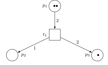
Fig. 1 Example of a Place Transition Net.
4 Extending Place Transition Nets
Our endeavour hereafter will focus on reducing the number of decision variables re-quired by an ILP to solve a mixed auction WDP. Along this path we start in this section by introducing a new optimisation problem on an extension of Place Transi-tion Nets. In SecTransi-tion 5 we show how instances of the WDP for mixed aucTransi-tions can be transformed into instances of the optimisation problem described in this section. As a result of such transformation we manage to reduce the number of decision variables from quadratic to linear in the number of operations.
In this section, we first introduce Place Transition Nets to subsequently extend them to incorporate a value function. We call the resulting model Weighted Place Transition Nets. Afterwards, we define a new optimization problem on Weighted Place Transition Nets, the Constrained Maximum Weighted Occurrence Sequence Problem. Finally, we explain how to solve such an optimization problem (in some special cases) by means of Integer Linear Programming.
4.1 Petri Nets and Place Transition Nets
Petri Nets are a powerful mathematical and graphical tool for the description of discrete distributed systems. They were first introduced in 1962 by Karl Adam Petri in his seminal dissertation [26]. In particular they are suitable for describing systems in which parallelism, concurrency, and synchronization play an important role. We refer the reader to [7] for a very good review.
We will focus on a particular type of Petri net called Place Transition Net. In the following we refer to Place Transition Net asnetfor short. Formally, following [7]:
Definition 3 (Place Transition Net Structure)APlace Transition Net Structure is a tupleN = (P, T, A, E) whereP is a set ofplaces,T is a finite set of transitions such thatP∩T =∅,A⊆(P×T)∪(T×P) is a set ofarcs, andE:A→N+ is anarc expression function (E(t, p) stands for the number of tokens introduced by transition tinto placepandE(p, t) stands for the number of tokens substracted from placepby
transitiont). ⊓⊔
In the following, we use the term structure to refer to a Place Transition Net Structure for short.
[image:10.612.150.337.36.152.2]Definition 4 (Marking)Amarking M:P→Nof a structure is a multiset overP. M(p) =kmeans that placep∈P containsktokens for markingM. ⊓⊔
A net is a structureS together with a given initial markingM0. An example of net is shown in Figure 1. The graphical representation of a net is composed of the following graphical elements: places (drawn as circles), transitions (drawn as rectangles), arcs (connecting places to transitions or transitions to places) labelled with values of an arc expression functionE. Tokens are drawn as bullet points inside the circles representing places.
Given a markingM, we say that a transition isenabledif all its input places contain at least as many tokens as required by the the transition’s input arcs. Intuitively, a transition is enabled if enough tokens are present in its input places. In other words, a transitiont∈T is said to beenabled if each input placepoftis marked with at least E(p, t) tokens, whereE(p, t) represents the weight of the arc connectingpto t. More formally,
Definition 5 (Enabled Transition) Given a marking M, a transition t ∈ T is
enabled iffM(p)≥E(p, t) ∀(p, t)∈A. ⊓⊔
If a transition is enabled it can fire consuming the tokens specified by E of the input places and producing the tokens specified byEin the output places. An enabled transition may or may not fire. If it fires, it changes the current marking to a new marking by removing tokens from the input places and putting tokens into the output places. More formally:
Definition 6 (Firing of an enabled transition)Thefiringof an enabled transition t removesE(pi, t) tokens from each input placepi and addsE(t, po) tokens to each output placepo. The firing of a transitiontchanges markingMk−1to a markingMk. The new marking can be computed employing the following equation:
Mk(p) =Mk−1(p) +E(t, p)−E(p, t) ∀p∈P (7)
Note that in this equation and henceforth, for simplicity, we assume thatE(p, t) = 0
if (p, t)6∈AandE(t, p) = 0 if (t, p)6∈A. ⊓⊔
4.1.1 Reachability
Recall that any WDP for a mixed auction defines an initial multiset of goodsUinand a final multiset of goodsUout. Hence, we can think of the problem as reaching Uout starting from Uin. There is a similar problem in nets: the problem ofreachability. It studies whether we can reach a particular state of a net departing from a given initial state only by using a sequence of net transitions.
Definition 7 (Firing Sequence) Given a structureS and a markingM0, a firing sequence is a sequence of transitionsht1, t2, . . . , tdifromS such thatt1is enabled in
M0and for alli∈[2, d],ti is enabled after firingti−1. ⊓⊔
By the repeated application of equation (7) a firing sequence J =ht1, t2, . . . , tdi brings markingM0 toMd:
Md(p) =M0(p) + X
t∈J
Definition 8 (Reachability)A markingMd isreachablefrom a marking M0 in a structureS if there exists a firing sequence that transformsM0intoMd. ⊓⊔
All the markings reachable from M0 in a structureS are writtenR(S,M0), and are called thereachable set of a net.
4.1.2 Reachability and the state equation
In the general case Lipton [27] proved that the reachability problem is EXPSPACE-hard. And yet, it is reasonable to wonder whether there are special classes of nets on which reachability is computationally simpler. In this section we show that indeed computation is simpler for a particular topology of nets by relying on results proved in [7].
Given a net with r transitions and nplaces, its incidence matrix A = [aij] is an r×nmatrix of integers. Each entry is given byaij =E(ti, pj)−E(pj, ti). Hence,aij is the difference in the number of tokens in placejwhen transitionifires once.
We can represent a markingMk as ann×1 column vectorMk such that thej-th entry ofMkrepresents the number of tokens present in placepj. We can identify each transitionti with afiring vector uti, anr
×1 column vector having a 1 at positioni and zeros elsewhere. We can now express equation (7) in matrix form as:
Mk=Mk−1+ATut (9)
whereAT stands for the transpose of incidence matrixA.
Given a firing sequenceJ=ht1, . . . , tdi, itsfiring count vectorKJis anr×1 column vector containing at thei-th position the number of times that thei-th transition in T is repeated in sequenceJ. Formally,KJ =Pd
k=1ut k.
Say that Md is reachable from M0, then there exists a firing sequence J =
ht1, t2, ..., tdibringing from markingM0to Md. Therefore, anecessary condition on reachability can be expressed in terms of a matrix equation:
Theorem 1 (Murata,1989) IfMd is reachable fromM0, then the following equa-tion has a non-negative integer soluequa-tionx:
Md=M0+ATx (10)
The proof consists in showing thatx=KJ is a solution. Notice that thei-th entry of vectorxencodes the number of times a transitionti must be fired to transformM0 intoMd.
Equation (10) is called the state equation, since it describes the states that a net would reach if the transitions encoded in x were fired. However, notice that the condition is not sufficient because the existence of a solution does not always imply thatMd is reachable fromM0. However, we can show that sometimes all the states reachable by a net are described by the state equation. In particular, this happens when the net is acyclic.
Definition 9 (Acyclicity) Adirected cycle in a structure (P, T, A, E) is a sequence of places and transitions hp1, t1, p2, t2, . . . , tn−1, pni such that p1 = pn and for all i∈[1, n] we have that (pi, ti)∈Aand (ti, pi+1)∈A.
In [7], it is shown that in anacyclicnet, the condition expressed by Theorem 1 is not only necessary, but also sufficient to guarantee reachability.
Theorem 2 (Murata,1989) In an acyclic structure (P, T, A, E), Md is reachable fromM0 iff the following equation has a non-negative integer solution inx:
Md=M0+ATx (11) That is, for any acyclic net, if there exists a solution to equation (11), a firing sequence reaching Md from M0 is guaranteed to exist, and x represents its firing count vector.
Moreover, Murata further extends the class of nets for which the condition is still sufficient. These particular nets (trap-circuit and syphon-circuit nets) have special topologies with particular types of circuits. For such nets, the state equation represents all the reachable states if the initial marking M0 satisfies some constraints. Further efforts have been made for extending the validity of the state equation to more classes of nets [28].
4.2 Weighted Place Transition Nets
There is a feature of some discrete systems (in particular the ones we consider) that, to the best of our knowledge, has never been considered so far in the Petri net literature, and that we deem as fundamental. A change in the state of a system may have an associated value. For instance, in our case, an operation has an associated value every time it is performed. Thus, in order to model operations, we need to extend nets to incorporate the notion of transition value. Such extension will allow us not only to represent the fact that a value is associated with each transition firing, but also to easily compute the value of afiring sequence.
We extend the notion of net (see Section 4.1) by attaching avalueto each transition. This leads us to the definition ofWeighted Place Transition Net StructureandWeighted Place Transition Net (henceforth referre to as weighted structure and weighted net respectively for short).
Definition 10 (Weighted Structure)A weighted structure is a a tuple (P, T, A, E, V) where:
– (P, T, A, E) is a structure.
– V :T →Ris a function that assigns a value to each transition.
⊓ ⊔
We define a weighted net by associating to a weighted structure an initial marking M0.
The initial marking in a net represents the initial state of the system, the very same semantics is inherited by weighted nets.
Weighted structures and weighted nets preserve all the properties of structures and nets respectively, but allow the quantitative representation of the value of a transition. Therefore, we can naturally apply to them all the concepts employed for nets. Those include the concepts of enabling of a transition, firing of a transition, marking, firing sequence, and so on.
Definition 11 (Value of a firing sequence)The valueV of a firing sequenceJ= ht1, t2, ..., tdiis the sum of the values of each transition contained in the sequence:
V(J) = d X
i=1
V(ti) (12)
⊓ ⊔ If a transition fires more than once, say k times, then its value will be added k times.
4.2.1 Constrained Maximum Weight Occurrence Sequence Problem
Since each transition has a value, it is reasonable to wonder about the optimal firing sequence leading from an initial marking to some final marking. Moreover, and more generally, we may require to compute the optimal firing sequence leading from an initial markingM0to a final markingMdthat fulfils some constraints. For instance, a given problem may require that each place in the final marking contains at least one token (Md(p)>1,∀p∈P). In order to model this more general optimisation problem, we define theConstrained Maximum Weight Occurrence Sequence Problem (MAXSEQ).
Definition 12 (MAXSEQ) Given – a weighted netN = (P, T, A, E,M0, V),
– a set of inequality constraints over a subset (P≥) of the places of a markingMd, expressed as:
∀p∈P≥ Md(p)≥gp, (13)
– and a set of equality constraints over a subset (P=) of the places of a marking Md, expressed as:
∀p∈P= Md(p) =hp (14)
find a firing sequenceJopt=ht1, t2, ..., tdithat maximizes the sequence valueV among the ones that bring from some initial markingM0to a final markingMd that fulfills
the constraints in equations (13) and (14). ⊓⊔
4.2.2 Reducing MAXSEQ to ILP
result also shows that the final markingMd in term of which the constraints are ex-pressed, is a linear function ofx(sinceMd=M0+ATx). This result can be extended to weighted nets without changes and is the basis for our ILP program.
Notice also that the function to maximize, (that is, the value of each firing sequence) does not depend on the order of the sequence (see equation (12)). Furthermore, since a value is associated to each transition in the net, the value depends linearly on the number of times each transition fires. We define a vectorv∈R|T|whosej-th position represents the value associated with transition tj (v[j] = V(tj)). Hence, the value associated with the firing sequence represented byx, is:
V(x) =vTx (15)
Now that we have shown the connection between MAXSEQ and ILP, we can for-mally state it.
Theorem 3 Given a MAXSEQ instance formed by a weighted net(P, T, A, E,M0, V) with incidence matrixAand the constraints appearing in equations (13)and (14):
If the state equation describes all the reachable states of the weighted net, then all the non-negative integer solutionsx of the following ILP:
max vTx (16)
subject to ∀p∈P≥ Md(p)≥gp (17)
∀p∈P= Md(p) =hp (18)
where Md=M0+ATx (19)
represent the firing count vectors of all the optimal solutions to the MAXSEQ instance.
Proof Notice that equation (19) computes the final marking as a linear function ofx. Since the state equation describes all the reachable states,Md will range over every possible final marking. Then equations (17) and (18) directly translate the constraints in equations (13) and (14) in MAXSEQ. Finally, equation (16) computes the value of the firing sequence as given by (15). As a result, a solutionx∗ to the ILP defined by equations (16)-(19) optimizes the sum of the values associated with fired transitions while ensuring that the final marking is reachable and fulfils the constraints defined by
the MAXSEQ instance. ⊓⊔
Note that the number of integer variables required to solve MAXSEQ via ILP is exactly|T|, that is, the number of transitions of the net.
According to the results stated in Theorem 2, it is possible to express the reacha-bility set with the state equation when the net is acyclic. Then, we apply this result to MAXSEQ via the following corollary:
Corollary 1 Provided that a net is acyclic, every MAXSEQ defined on it can be re-duced to ILP.
Hence, every MAXSEQ instance over the net can be solved in two steps. First, we determine the optimal firing count vectorxopt by solving the ILP in equations (16)-(19). Then, since the net is acyclic, we can establish a partial order among transitions so thatt1≺t2ifft2uses as input some output oft1. We can construct an occurrence sequence Jopt by ordering the transitions in xopt non-decreasingly according to our partial ordering. In that way, every step inJoptis guaranteed to be enabled and
con-sequentlyJoptis a solution to the MAXSEQ instance. ⊓⊔
5 Mapping mixed auctions to weighted nets
In this section we demonstrate that an instance of the mixed auction WDP can be transformed into an instance of the MAXSEQ problem introduced in Section 4.2.1. Notice that this mapping allows us to benefit from analysis methods to study behavioral properties of Petri nets. Hence, we exploit such analysis methods to provide an ILP formulation for some classes of weighted nets, and therefore some types of supply chain networks.
5.1 Intuitions behind the mapping
The idea behind the mapping is that an atomic operation can be regarded as a tran-sition in a weighted net. Consider the following offer, expressed by a bidder in the bidding language introduced in Section 3.1:
Bid1=bid(1′(2′H2O,1′O2+ 2′H2),−8) (20)
This represents an offer to perform an hydrolysis process: 2 moles of water are transformed into 1 mole of oxygen and two moles of hydrogen at a price ofe8. Now consider the transition depicted in Figure 2, and say that each place represents a good. Let the place labelled withH2Obe water, H2 be hydrogen, and O2 be oxygen. The transition in Figure 2 perfectly captures the semantics of a supply chain operation: the input places of the transitions are the input goods of the operation, its output places are the output goods of the operation, and the transition value is the value associ-ated with the operation. Analogously, an operation offering goods can be represented as a transition with only output places, whereas an operation requesting goods as a transition with only input places.
Example 1 Say that the following bids are submitted to a mixed auction:
bid1=bid(1′({ },2′H2O),−10) (21)
bid2=bid(1′({ },2′H2O),−14) (22)
bid3=bid(1′(2′H2O,1′O2+ 2′H2),−8) (23)
bid4=bid(1′(2′H2+ 1′O2,{ }),23) (24)
bid5=bid(1′(2′H2+ 1′O2,{ }),25) (25)
O2 H2
H2O
Bid1
e8 2
1
2
Fig. 2 Example of an operation represented as a transition in a weighted net.
bid1 e−10 bid2 e−14
bid4
e23 e25 bid5
O2 H2
H2O
bid3
e−8 2
1
2 2
2
1 2
1
2
Fig. 3 Example of bids in a mixed auction represented as a weighted net.
Finding the revenue-maximizing solution in example 1 is straightforward. Firstly, buy two moles of water frombid1, then process the water through the operation inbid3, and then sell the products of the reaction tobid5. The total revenue of the supply chain is 25−8−10 =e7. Notice that this is also the solution to the MAXSEQ problem3 defined on the weighted net in Figure 3 with an empty initial marking and with a destination markingMd satisfying the following constraints:
Md(H2O)≥0 (26)
Md(O2)≥0 (27)
Md(H2)≥0 (28)
Given the example above, we argue that if we construct a MAXSEQ instance by:
1. building a weighted net joining all the atomic operations received within bids;
3
[image:17.612.128.360.40.157.2] [image:17.612.98.394.182.390.2]2. setting the initial marking to the goods initially available to the auctioneer (Uin); and
3. setting some constraints on the final marking (Uout),
then the solution to the MAXSEQ instance corresponds to the solution to the mixed auction WDP.
Nonetheless, we must take some more details into account. Firstly, in the previous example, given the weighted net representation, each operation can be used an arbi-trary number of times. Instead, the semantics of the bidding language imposes that operations must be used a limited number of times. Secondly, we must provide bidders with the capability of encoding on the weighted net both offers or requests over bundles of operations. Moreover, they also require the capability of encoding on the weighted net sets of mutually exclusive (XOR) atomic bids. Addressing these three issues is the purpose of the following section.
5.2 Representing Bids
In Example 1, we restricted ourselves to the case in which agents can only submit one atomic bid. Moreover, we only consider bidding over a single atomic operation, i.e. |Dij| = 1. Next, we progressively relax all these constraints. First of all, we explain how to represent a weighted net a bid on a bundle (multiset) of operations.
5.2.1 Expressing bids on bundles of operations
Given an atomic bidBidij, combinatorial on operations, we have to ensure that:
– if an atomic operationtijk in bidBidij is included in the solution sequence,
– it must be included in the solution as many times as required by the multiplicity oftijkin the bid (Dij(tijk));
– all the other atomic operationstijk′ within the same atomic bid (all the opera-tions inDij) must be included as many times as required by their multiplicities (Dij(tijk′)) as well;
– the money that the bidder must pay (receive) is the price of the whole bid (pij). Recall that bidder constraint 1.a) in Section 3.2 imposed that if a bidder submits an offer over a bundle of operations, all of them must be employed in the operation sequence. This is precisely what the first condition above captures.
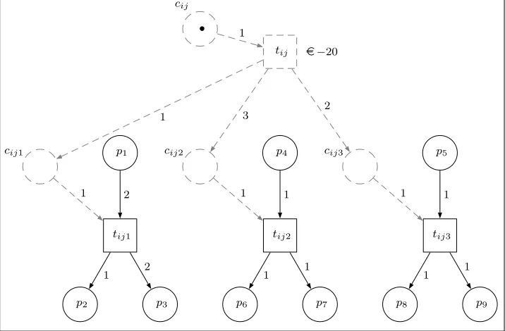
We achieve this by introducing some auxiliary places and transitions. The example in Figure 4 represents the following bid:
Bidij=bid(1′tij1+ 3′tij2+ 2′tij3,−20)
wheretij1= (2′p1,1′p2+ 2′p3),tij2= (1′p4,1′p6+ 1′p7) andtij3= (1′p5,1′p8+ 1′p9).
In general, in order to incorporate a bid over multiple operations we proceed as follows:
– for each bidBidij we introduce an auxiliary transitiontij (bid transition) and an auxiliary placecij (bid place).
tij3
tij2
p2 p3
p1 p4 p5
p6 p7 p8 p9
tij1
2
1 2
1 1
1 1 1 1
cij1 cij2 cij3
•
cij
tij e−20
1 1 1
1
1 3 2
Fig. 4 Bids on bundles of operations.
– we attach the valuation pij of bid Bidij to the corresponding bid transition tij. In the example, we associate the bid value pij=−e20 to transition tij. Hence, whenevertij fires, the cost/valuepij is added to the value of the firing sequence.
It is easy to check that the weighted net in Figure 4 allows to fire any subset of {tij1, tij2, tij3} (depending on the tokens) with the corresponding multiplicities (1,3,2). Notice also that firing at least one of the three transitions requires to pre-viously fire transition tij, because this guarantees having the required tokens in the input places cijk. In this way, we guarantee that firing at least one of the transitions implies firing also tij, and therefore that the corresponding money is added to the overall cost/value.
Any legal firing sequence on the weighted net in Figure 4 guarantees that selecting at least one of thetijk implies also selectingtij. However, we need a further require-ment: either none of thetijk fires, or all of them fire. If they all fire, they have to fire as many times as expressed by their multiplicities in the bids. In the figure, we have to enforce that if tij fires, then tij1 fires once (Dij(tij1) = 1),tij2 fires three times (Dij(tij2) = 3), andtij3fires twice (Dij(tij3) = 2).
The weighted net in Figure 4 cannot guarantee such property by itself. For instance, a firing sequence in which only transitions tij1 and tij2 fire (not tij3) is legal but does not comply with our all-or-nothing assumption. In order to enforce it, we simply impose some constraints on the final configuration of the net. Say that we impose that in the final configurationcij1, cij2, andcij3contain no tokens. More formally, the final marking should fulfil the constraints:
Md(cij1) = 0 (29)
Md(cij2) = 0 (30)
[image:19.612.69.427.32.267.2]This implies that all the legal firing sequences leading to the final configurationMd contain either none or the three transitionstij1, tij2, tij3 with multiplicities 1, 2, and 3 respectively.
Therefore, the semantics regarding the multiplicity of the operations offered in bid Bidij is completely captured by the weighted net provided. Furthermore, the weights of the arcs connecting each bid transitionstij with its operation placescijk, along with the constraints on the final marking, enforce that either none of the operations inDij is used, or all of them are used as many times as indicated by their multiplicities in Dij.
The following proposition formalises how a weighted net structure as constructed above can capture the semantics of an atomic bid.
Proposition 2 LetBidijbe an atomic bid with valuepijand its corresponding weighted structure (P, T, A, E, V)with initial markingM0(cij) = 1, andM0(cijk) = 0for all operation places. If any final marking Md is required to fulfil thatMd(cijk) = 0 for all operation places, then any legal firing sequence fires either all or none of the atomic operations in the bid, being pij the value of the firing sequence in the first case and 0 otherwise.
Proof Since M0(cij) = 1, bid transition tij is enabled and thus can be fired. We distinguish two cases at this point. On the one hand, iftij does not fire, none of the atomic operations can fire, the constraints on the final marking hold and the value of not firingtij is 0. On the other hand, iftijfires, then each operation placecijkreceives Dij(tijk) tokens from transitiontij. Since each transitiontijk requires a single token to be enabled, all atomic transitions are enabled. Since we have imposed that the final markingMd leaves no tokens at the operation places, namelyMd(cijk) = 0 ∀cijk, all atomic transitions must fire. Therefore, both the bid transitiontij along with all atomic transitionstijkcompose the firing sequence. Since firing atomic transitions has no cost, the value of the firing sequence is V(tij) = pij, which is the value of bid
Bidij. ⊓⊔
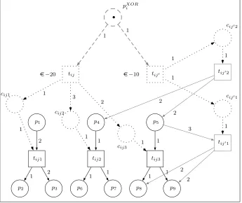
5.2.2 Expressing XOR of atomic bids
We have learnt how to represent an atomic bid on a weighted net. However, we still have to encode the XOR relationships among the atomic bids that come from each bidder to fully represent our bidding language. Consider the following bid:
bid(1′tij1+ 3′tij2+ 2′tij3,−20) XOR
bid(1′tij′1+ 1′tij′2,−10)
where tij1= (2′p1,1′p2+ 2′p3), tij2 = (1′p4,1′p6+ 1′p7), tij3 = (1′p5,1′p8+ 1′p9), tij′1= (3′p5,2′p8+ 2′p9), andtij′2= ({ },2′p4+ 2′p5).
Hereafter we refer to the two bids above submitted by some bidderiin XOR as to Bidij andBidij′. Figure 5 depicts bidsBidij andBidij′.
p2 p3
p1 p4 p5
p6 p7 p8 p9
tij1 tij2 tij3
2
1 2
1 1
1 1 1 1
tij′1
3
2
2
tij′2
2 2
cij1
cij2
cij3
cij′1
cij′2
tij
e−20 e−10 tij′
1
1
1 1
3
2
1
1 1
1 •
pXOR
i
1 1
Fig. 5 XOR of atomic bids.
enforced to contain a single token by the initial marking. Hence, the resulting weighted net topology enforces that at most one of the atomic bids in XOR is selected. In figure 5 eithertij or tij′ can fire, but not both. When either of them fires, it consumes the unique token in pXORi , thus preventing the firing of the other one. This corresponds to selecting at most one bid out of bidsBidij and Bidij′. This reasoning naturally applies to the general case of m bids in XOR. Moreover, say that, for instance, we choose to fire tij. Then all atomic operations in the bid (namely tij1, tij2, tij3) must fire as stated by proposition 2. In other words, anXOR place acts as an exclusive bid place for all the atomic bids involved in an XOR bid.
5.3 Connecting the mixed auction WDP and MAXSEQ: the Mixed Auction Net
In this section we formalize what was explained informally in the previous section: how to build a weighted net that encodes all the bids received by an auctioneer. We shall call such weighted net theMixed Auction Net.
[image:21.612.72.417.44.334.2]Algorithm 1 details how to build a mixed auction net from some setBof XOR bids. Line 1 creates a place for each good at auction and initialises the remaining variables to empty sets. We callPGthe set that contains the places that represent goods. Lines 2-4 establish that the initial marking for places that represent goods is set according to the number of units thatUinspecifies for each good. Line 7 adds a new place (pXORi ) for each XOR bid and adds a single token (unit) to the initial marking (so that each XOR bid can be only selected once). ThePXORset contains all XOR places. Line 10 adds a new transition (tij) for each atomic bid and sets its value topij (the value specified by the bid), whereas line 11 links each newly created transition with the place representing its XOR bid. Line 13 adds acontrol placecijk to control each operation and line 14 links it as an output to the transition representing its combinatorial bid (tij), setting the number of tokens to output to the cardinality of operationtijkin the combinatorial bid (namely toDij(tijk)). ThePC set contains all the control places. Line 16 adds a new transition tijk (with value zero) for each atomic bid, which line 17 links to its control placecijk so that each timetijk fires, it consumes a token fromcijk. We call the set of all transitions representing operations TOP. Finally, lines 18-20 and 21-23 link each transition tijk representing an operation with its input and output goods respectively.
The introduction of the mixed auction net allows us to define the mixed auction WDP as a MAXSEQ problem.
Theorem 4 Given a mixed auction with a multiset of available goodsUin, a multiset of required goods Uout, and a set of bids B in the XOR language over the goods in G, solving the WDP amounts to solving the MAXSEQ problem defined on the Mixed
Algorithm 1ConstructMixedAuctionNet(B,Uin)
1: P← {pg| g∈G};T ← ∅;A← ∅;M0← ∅;
2: forginGdo
3: M0← M0+{Uin(pg) copies ofpg}; /* Establish initial marking for goods */
4: end for
5: forBidiinBdo
6: /* Add a place for each XOR bid and set its initial marking to contain one token */ 7: P ←P∪ {pXOR
i };M0← M0+{pXORi };
8: forBidijinBidido
9: /* Add a new transition for each atomic bid, set its value to the bid’s value */ 10: T ←T∪ {tij};V(tij) =pij;
11: A←A∪ {(pXOR
i , tij)};E(pXORi , tij) = 1; /* and link it to its XOR bid */
12: forBidijk inBidijdo
13: P←P∪ {cijk}; /* Add a new place for each operation */
14: A←A∪ {(tij, cijk)};E(tij, cijk) =Dij(tijk); /* and link it to its combin. bid */
15: /* Add a new transition for each operation, set its value to zero */ 16: T ←T∪ {tijk};V(tij) = 0;
17: A←A∪ {(cijk, tijk)};E(cijk, tijk) = 1; /* link it to its control place, */
18: forginIijkdo
19: A←A∪ {(pg, tijk)};E(pg, tijk) =Iijk(pg); /* link it to its inputs */
20: end for 21: forginOijkdo
22: A←A∪ {(tijk, pg)};E(tijk, pg) =Oijk(pg); /* and link it to its outputs */
23: end for 24: end for 25: end for 26: end for
Auction Net S = (P, T, A, E,M0, V) with destination marking Md that fulfils the following constraints
Md(p)≥ Uout(g) p∈PG (32)
Md(p) = 0 p∈PC (33)
Md(p)≥0 p∈PXOR (34)
Proof The proof is long and needs a bit more notation than introduced in this paper. We only report about the way the two solutions can be mapped to each other. For the complete proof the reader can consult [25].
⇒) First, we prove that a solution to MAXSEQ can be transformed into a solution to the WDP. Note that each solution to MAXSEQ is a sequence of transitions, some of them representing atomic bids and some others representing operations. A solution to the mixed auction WDP is composed by two sets of binary variablesxmijk (that takes on 1 iftijk is at positionm in the solution sequence) andxij (that takes on 1 if bid Bidij is accepted). We construct the mixed auction WDP solution by removing from the MAXSEQ solution all the transitions that represent atomic bids. In the resulting sequence, transitions only represent operations. Hence, we can set to 1 those variables xmijk such that operationtijk appears at positionm. Regarding the transitions in the MAXSEQ solution that represent atomic bids, we can setxij to 1 iftij appears in the MAXSEQ solution. It is then straightforward (although tedious and beyond the scope of this paper) to show that this assignment of values toxmijk andxij fulfils the conditions in equations (1)-(6) corresponding to the Direct Integer Program that solves the MMUCA WDP.
⇐) We prove the converse as well. Given a solution {xmijk,xij}to the mixed auction WDP, it can be transformed into a solution to the MAXSEQ problem posed in the theorem. In this case we construct a sequence of transitions by placing a transitiontij (representing an atomic bid) in the sequence for each bidBidij such thatxij is 1. We can place these transitions at any order at the beginning of the sequence. We complete the remainder of the sequence with transitions that represent operations following the order specified by xmijk. More precisely, ifk atomic bids are selected for the solution (k variablesxij taking on 1), then for every variablexmijk with value 1 we can place the transition representing operationtijkat positionk+mof the transition sequence. It is also tedious but simple to show that such sequence fulfils the conditions to be a
solution to the MAXSEQ problem. ⊓⊔
Notice that it is straightforward to generalise the previous result for the OR lan-guage by incorporating appropriate changes to the weighted net. Thus, we should only represent all the bids as in Figure 4, omitting the XOR places.
Now we can start benefitting from Theorem 4 by providing (under acyclicity) a better mapping of the mixed auction WDP to ILP than the one provided in Section 3.3.
Corollary 2 Whenever a mixed auction net is acyclic, the mixed auction WDP can be reduced to ILP using|B|+|T|variables, where |B|stands for the number of atomic bids received and |T| stands for the number of different operations appearing in the bids.
Proof Follows directly from the fact that the mixed auction WDP can be reduced to MAXSEQ and that whenever the weighted net is acyclic MAXSEQ can be reduced to
Recall that the number of variables needed for the mapping in Section 3.3 isO(δ· |T|), i.e. it is quadratic in|T|, and possibly even significantly larger than that, namely when transformations appear with high multiplicity. The acyclicity constraint excludes some interesting cases such as those where a good is borrowed and returned after the execution of the operation. However, it covers some common topologies such as the assembly of a good from its components or its dissasembly into its parts (though not both simultaneously).
Our aim in this section is showing that, from the firing sequence associated with a particular MAXSEQ problem on theMixed Auction Net, we can derive an optimal solution sequence to the corresponding mixed auction WDP.
5.4 Advantages of the mapping to MAXSEQ
It is time to highlight the advantages brought about by mapping the mixed auction WDP to the MAXSEQ problem over weighted nets. In particular, the mapping allows to import all the Petri net tools and properties presented in the literature to analyze structural and behavioral properties of the supply chain resulting from a mixed auction. Some examples of application are listed below:
1. One can very efficiently solve the underlying ILP when the supply chain is acyclic. This benefit comes from exploiting an important nets analysis tool, the state equa-tion.
2. One may be interested in maintaining under a certain threshold the level of re-sources present in each place (for instance, because of inventory capacity con-straints). In order to guarantee that resources do not exceed some threshold(s) amounts to investigating the so-called boundedness property [7], a well-known be-havioural property of nets.
3. Due to the very appealing and intuitive weighted net graphical representation, we can compactly encode and visualize the search space associated with the mixed auction WDP. This stems from the the fact that the semantics of transitions on nets naturally accommodates the representation of operations.
4. Once a solution sequence to the mixed auction WDP is obtained, one can visualize it by means of a token game showing the evolution of the supply chain at any step of the operation sequence.
5. One can graphically visualize the mixed auction WDP problem. This provides a very helpful guidance to obtaine insights about the problem. For instance, by visualizing the mixed auction WDP by means of a weighted net, one can incorporate new bidding language constructs with a minimum effort. For instance, consider the following example.
Example 2 We explained that switching to theOR language instead of theXOR bidding language is as simple as removing theXORplace from Figure 5, as shown in Figure 4. However, there is another widely employed bidding language that is very compact and human-readable. Is is called the XOR-of-OR bidding language (refer to Section 3.1). When employing a XOR-of-OR bidding language, any XOR combination of OR combinations of atomic bids can be selected. For instance, the following bid:
means that an auctioneer can select from 0 to 5 copies of atomic bid (a,1) or one copy of atomic bid (b,2), but not both things at the same time. In Figure 6, we graphically show how to incorporate theXOR-of-ORbidding language by depicting the following bid:
(bid(1′tij1+ 3′tij2+ 2′tij3,−20) OR (36)
bid(1′tij′1+ 1′tij′2,−10))XOR (37)
bid(1′tij′′1,−2) (38)
tij1 tij2 tij3
tij′1
tij′2
= 0
cij1
= 0
cij2
= 0
cij3
= 0
cij′1
= 0
cij′2
tij
e−20 e−10 tij′
1 1 11
1 3
2
1
1 1
1 1 •
pXOR
i
≥0
≥0 ≥0
tOR ij′
tij′′1
= 0
cij′′1 tij′′
e−2
1
1
1 1
1 1
1 1
Fig. 6 XOR-of-OR of atomic bids
The single token in placepXORi allows either to fire transitiontij′′ or (exclusively) transition tORij′ . If transitiontij′′fires, then the auctioneer would be using the bid
[image:25.612.64.412.139.470.2]6 Conclusions and future work
Mixed auctions can potentially be employed for the automated assembly of supply chains of agents. However, in order for mixed auctions to be effectively applied to SCF, we must ensure computational feasibility while preserving optimality. In this paper we have tried to make headway along this direction.
Firstly we discussed the notions of bidding language and winner determination for mixed auctions following [4]. Integer programming allows to solve the mixed auction WDP onanysupply chain network topology. However, it has the disadvantage to be computationally expensive. In fact, such a an ILP formulation requires a number of decision variables that grows quadratically with the number of operations mentioned in the bids. This computational cost motivates the need for efficient solvers that support the practical application of mixed auctions.
Contributions on computationally efficient WDP solvers for different auction types (namely, [22] for CAs and [29] for multi-attribute double auctions) agree on and defend that a careful, formal analysis of the structure of the WDP can provide guidance for developing efficient solvers. Along this line we have introduced a graphical formalism that allows to compactly represent both the search space and the solutions associated with the mixed auction WDP. To attain this goal we have extended Place Transition Nets to provide the so-called weighted nets, we have defined a new optimisation problem over weighted nets, the so-called Constrained Maximum Weight Occurrence Sequence Problem (MAXSEQ), and we have mapped the mixed auction WDP to a MAXSEQ. Notice that the validity of the mapping from the mixed auction WDP to weighted nets is not restricted to bids in the XOR language, but in fact it can easily cope with other languages. For instance, as discussed in Section 5.4, the extension to the OR and the OR-of-XOR language is trivial.
A major benefit of our graphical formalism is that it allows to formally analyse the structural and behavioural properties of the mixed auction WDP. In this work, as a first result of our structural analysis, we demonstrate how to dramatically reduce the number of decision variables (from quadratic to linear with respect to the number of operations) for a broad class of mixed auctions WDPs (in particular, when the weighted nets underlying the mixed auction WDP is acyclic).
Notice that although our approach is limited to a class of mixed auction WDPs, we know from the literature that it is possible to increase the classes of Petri nets for which the state equation represents the whole reachability set. As an example, one may add linear side constraints to the state equation [30]. In general, we would like to broaden the class of mixed auction WDPs we can efficiently solve. Thus, our future aim will be to devise the most efficient solver for each class of mixed auction WDP.
Acknowledgements
We would like to thank the anonymous reviewers for their extensive and helpful com-ments. This work was funded by the Jose Castillejo programme (JC2008-00337), IEA (TIN2006-15662-C02-01), OK (IST-4-027253-STP), eREP(EC-FP6-CIT5-28575) and Agreement Technologies (CONSOLIDER CSD2007-0022, INGENIO 2010).
References
1. P. Cramton, Y. Shoham, R. Steinberg (Eds.), Combinatorial Auctions, MIT Press, 2006. 2. W. E. Walsh, M. P. Wellman, F. Ygge, Combinatorial auctions for supply chain formation, in: EC ’00: Proceedings of the 2nd ACM conference on Electronic commerce, ACM, New York, NY, USA, 2000, pp. 260–269.
3. W. Walsh, M. Wellman, Decentralized supply chain formation: A market protocol and competitive equilibrium analysis, Journal of Artificial Intelligence Research 19 (2003) 513– 567.
4. J. Cerquides, U. Endriss, A. Giovannucci, J. A. Rodriguez-Aguilar, Bidding languages and winner determination for mixed multi-unit combinatorial auctions, in: Proc. of the 20th Intl. Joint Conferences on Artif. Intelligence (IJCAI), Hyderabad, India, 2007, pp. 1221–1226.
5. M. Vinyals, A. Giovannucci, J. Cerquides, P. Meseguer, J. A. Rodriguez-Aguilar, A test suite for the evaluation of mixed multi-unit combinatorial auctions, Journal of Algorithms 63 (1-3) (2008) 130–150.
6. A. Giovannucci, J. A. Rodriguez-Aguilar, J. Cerquides, U. Endriss, Winner determination for mixed multi-unit combinatorial auctions via petri nets, in: AAMAS ’07: Proceedings of the 6th international joint conference on Autonomous agents and multiagent systems, ACM, New York, NY, USA, 2007, pp. 710–717.
7. T. Murata, Petri nets: Properties, analysis and applications, in: Proceedings of the IEEE, Vol. 77, 1989, pp. 541–580.
8. T. Sandholm, S. Suri, A. Gilpin, D. Levine, Winner determination in combinatorial auction generalizations, in: AAMAS ’02: Proceedings of the first international joint conference on Autonomous agents and multiagent systems, ACM Press, Bologna, Italy, 2002, pp. 69–76. 9. C. Caplice, Y. Sheffi, Combinatorial Auctions for Truckload Transportation, MIT Press,
2006, Ch. 21. Combinatorial Auctions.
10. E. Cantillon, M. Pesendorfer, Auctioning Bus Routes: The London Experience, MIT Press, 2006, Ch. 22. Combinatorial Auctions.
11. M. Bichler, A. Davenport, G. Hohner, J. Kalagnanam, Industrial Procurement Auctions, MIT Press, 2006, Ch. 23. Combinatorial Auctions.
12. M. O. Ball, G. L. Donohue, K. Hoffman, Auctions for the Safe, Efficient, and Equitable Allocation of Airspace System Resources, MIT Press, 2006, Ch. 20. Combinatorial Auc-tions.
13. A. Pekec, M. H. Rothkopf, Combinatorial auction design, Manage. Sci. 49 (11) (2003) 1485–1503.
14. V. Krishna, Auction Theory, Academic Press, 2002.
15. P. Milgrom, Putting Auction Theory to Work, Cambridge University Press, 2004. 16. N. Nisan, Bidding Languages for Combinatorial Auctions, MIT Press, 2006, Ch. 9.
Com-binatorial Auctions.
17. M. H. Rothkopf, A. Pekec, R. M. Harstad, Computationally manageable combinational auctions, Management Science 44 (8) (1998) 1131–1147.
18. A. Andersson, M. Tenhunen, F. Ygge, Integer programming for combinatorial auction winner determination, in: Fourth International Conference on Multiagent Systems (ICMAS 2000), Boston, MA, 2000, pp. 39–46.
19. T. Sandholm, Algorithm for optimal winner determination in combinatorial auctions, Ar-tificial Intelligence 135 (1-2) (2002) 1–54.
21. K. Leyton-Brown, Y. Shoham, M. Tennenholtz, An algorithm for multi-unit combinatorial auctions, in: Proceedings of the American Association for Artificial Intelligence Conference (AAAI), 2000, pp. 56–61.
22. D. Lehmann, R. M¨uller, T. Sandholm, The winner determination problem, MIT Press, 2006, Ch. 12. Combinatorial Auctions.
23. R. M¨uller, Tractable Cases of the Winner Determination Problem, MIT Press, 2006, Ch. 13. Combinatorial Auctions.
24. T. Sandholm, Optimal Winner Determination Algorithms, MIT Press, 2006, Ch. 14. Com-binatorial Auctions.
25. A. Giovannucci, Computationally Manageable Combinatorial Auctions for Supply Chain Automation, Ph.D. thesis, Universitat Autonoma de Barcelona. Departamento de ciencias de la Computacion.http://specs.upf.edu/files/u20/Monografia.pdf. (2008). 26. C. Petri, Kommunikation mit Automaten.Univ. Bonn, Institut f¨ur Instrumentelle
Mathe-matik, Schriften des IIM Nr. 2, 1962., Tech. rep., English translation: RADC-TR-65-377, Griffiths Air Base, New York (1966).
27. R. Lipton, The reachability problem requires exponential space, Tech. Rep. 62, Yale Uni-versity (1976).
28. A. Tarek, N. Lopez-Benitez, Optimal legal firing sequence of Petri nets using linear pro-gramming, Optimization and Engineering 5 (1) (2004) 25–43.
29. Y. Engel, M. P. Wellman, K. M. Lochner, Bid expressiveness and clearing algorithms in multiattribute double auctions, in: EC ’06: Proceedings of the 7th ACM conference on Electronic commerce, ACM Press, New York, NY, USA, 2006, pp. 110–119.