Detection of abrupt baseline length changes using cumulative sums
Volker Janssen
School of Geography and Environmental Studies, University of Tasmania, Hobart, Australia [email protected]
Abstract
Dynamic processes are usually monitored by collecting a time series of observations, which is then analysed in order to detect any motion or non-standard behaviour. Geodetic examples include the monitoring of dams, bridges, high-rise buildings, landslides, volcanoes and tectonic motion. The cumulative sum (CUSUM) test is recognised as a popular means to detect changes in the mean and/or the standard deviation of a time series and has been applied to various monitoring tasks. This paper briefly describes the CUSUM technique and how it can be utilised for the detection of small baseline length changes by differencing two perpendicular baselines sharing a common site. A simulation is carried out in order to investigate the expected behaviour of the resulting CUSUM charts for a variety of typical deformation monitoring scenarios. This simulation shows that using first differences (between successive epochs) as input, rather than the original baseline lengths, produces clear peaks or jumps in the differenced CUSUM time series when a sudden change in baseline length occurs. These findings are validated by analysing several GPS baseline pairs of a network deployed to monitor the propagation of an active ice shelf rift on the Amery Ice Shelf, East Antarctica.
Keywords. Cumulative sum (CUSUM), GPS, baseline length changes, deformation monitoring, Amery Ice Shelf.
1. Introduction
The geodetic monitoring of dynamic processes is usually undertaken by acquiring a time series of measurements, which is then analysed in order to determine any motion or “abnormal” behaviour. Examples include the monitoring of dams, bridges, high-rise buildings, landslides, volcanoes and tectonic motion, and numerous geodetic networks have been established for these purposes. Depending on the task at hand and the risk involved in a potential “failure” of the structure being monitored, continuous monitoring and detection of changes in real time are often required to enable a fast response, e.g. initiating warning and/or evacuation procedures in case of an imminent volcanic eruption.
A popular technique for the detection of changes in the mean and/or the standard deviation of a time series is the cumulative sum (CUSUM) test, which was proposed by Page (1954) and has since been modified and extended to accommodate various conditions (e.g. Page 1957, Hinkley 1970, 1971, Lorden 1971, Lucas and Crosier 1982, Moustakides 2004).
investigate the expected behaviour of the resulting CUSUM charts, leading to a slight modification of the technique. Findings will be validated using GPS data collected at a propagating ice shelf rift.
2. How do cumulative sums work?
CUSUM algorithms are generally classified into two types. The one-sided CUSUM is applicable when both the means before and after a change are known, while the two-sided CUSUM is to be used when the change magnitude is unknown (generally the case in deformation monitoring applications).
2.1. One-sided CUSUM
Considering a time series of n independent and normally distributed observations, a cumulative function can be
defined as (Basseville and Nikiforov 1993):
( )
( )
1
0
1
with
ln
n
i
n i i
i i
p
x
S
z
z
p
x
µ µ =
=
=
(1)where zi is the log-likelihood ratio for the observation xi. The probability densities pµ0 and pµ1 before and after the
change, respectively, are defined according to:
( )
( )2 2
2
1
2
ix
i
p x
e
− −
=
µ σ
µ
σ π
(2)where σ2 is the variance of the observations (here assumed constant). Hence, the cumulative sum for the nth
sampling point can be expressed as:
0
1
2
n
n i
i
b
S
x
=
=
−
µ
−
δ
σ
(3)where δ = µ1–µ0 is the magnitude of the change between the mean values before and after the shift, and b = (µ1–
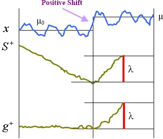
µ0)/σ is the signal-to-noise ratio. In the case of a positive shift in the mean, the above function typically shows a
negative drift before and a positive drift after the jump occurs. The situation is reversed when a negative shift in the mean is present.
The underlying assumption of the one-sided CUSUM test is that either a positive or a negative shift of known magnitude has occurred. In the case of a positive shift of the mean, the relevant information for change detection lies in the difference between the value of the log-likelihood ratio and its current minimum value. At each time
instant k, this difference is compared to an appropriately chosen threshold λ. An alarm will then be issued if this
threshold has been reached or exceeded (Basseville and Nikiforov 1993):
1min
k k t
t k
g + S S
λ
≤ ≤
= − ≥ (4)
where gk+ is known as the decision function for a positive shift. In essence, the cumulative sum is compared to an
Figure 1: Typical behaviour of the cumulative sum S + and decision function g + corresponding to a positive shift in the mean (adapted from Ogaja 2002).
2.2. Two-sided CUSUM
If the magnitude δ of a change in the mean value is known but it is not known whether a positive or negative
shift occurred, it is intuitive to apply the CUSUM test simultaneously in two directions. This implies that the
mean value after the shift has either increased to µ1+ = µ0 + | δ | or decreased to µ1– = µ0 – | δ |. An alarm will
then be issued either according to equation (4) or if:
1 max
k t k t k
g − S S
λ
≤ ≤
= − ≥ (5)
This corresponds to the well-known cumulative sum charts widely used for continuous monitoring or inspection
schemes. In practice, however, the magnitude of the shift is generally unknown. Three possible a priori choices
can be made with respect to this parameter (e.g. Basseville and Nikiforov 1993):
1) Choose δ as a minimum possible jump magnitude with | δ | > 0.
2) Choose δ as the most likely jump magnitude.
3) Choose δ as a worst-case value with regards to the impact or cost of an undetected jump.
In this context it should be noted that in most practical cases, particularly for real time applications, the time delay between the detection of a jump and the issuing of an alarm on the one side and the number of false alarms on the other need to be kept to a minimum. This obviously has implications on the CUSUM algorithm design for a given application but will not be discussed in this paper.
3. Differencing to detect baseline length changes
Recently a technique to reveal subtle changes in baseline length time series based on the analysis of CUSUM charts was proposed by Iz (2006), which is briefly described in this section. Forming the difference of two baselines that share a common site reduces common systematic errors and thereby allows the detection of small changes with better signal-to-noise ratios. If the two baselines run approximately parallel and perpendicular to the expected deformation, any hidden changes in the time series can be detected, although these changes will be reduced in magnitude as any common signal is removed in the difference.
negative slope is an indication of values being below the mean. A sudden shift in the mean of the time series
causes a sudden change in the slope sdiff. The magnitude of this sudden change, | sdiff |, can be estimated from (Iz
2006):
0 0
max min
diff i n i i n i
s S S
≤ ≤ ≤ ≤
= − (7)
In order to reduce the influence of common systematic errors, the CUSUMs of two baselines sharing a common site are then differenced. If these baselines are located approximately parallel and perpendicular to the expected deformation, the subtle baseline changes remain in the differenced residuals, although their magnitude will be reduced, and thus can be detected. Iz (2006) successfully applied this technique to GPS and VLBI time series for crustal motion studies in the Tokyo area, Japan. The detected baseline length changes were associated with an earthquake swarm and volcanic activity on Miyakejima Island.
It should be noted that not all change points representing a sudden change of slope can be attributed to deformation due to the remaining unmodelled errors present in the time series. Depending on the source and length of the time series, these errors may include solid earth tides, ocean loading, atmospheric pressure variations and baseline processing errors (e.g. GPS orbit errors, residual ionospheric and tropospheric delays). However, if a change point is identified in multiple baseline pairs, its presence can safely be assumed.
4. CUSUM simulation
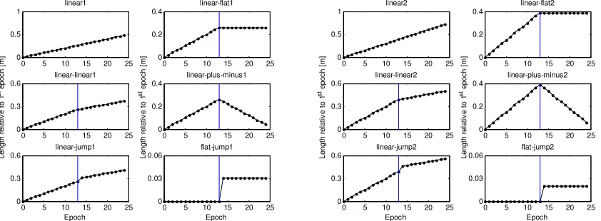
Several anticipated scenarios in a deformation monitoring situation were investigated by simulation of baseline time series in order to examine the expected behaviour of the resulting CUSUM charts. Cases considered included a uniform linear trend in baseline length, a change of the linear trend in a particular epoch, a change of the linear trend including a jump in baseline length, a linear trend changing to a constant baseline length, a linear increase-then-decrease situation, and a jump with constant baseline lengths on either side. For each of the two baselines, slightly different trends were chosen (Figure 2).
0 5 10 15 20 25
0 0.5
1 linear1
0 5 10 15 20 25
0 0.3
0.6 linear-linear1
Le
ng
th
r
el
at
iv
e
to
1
st e
po
ch
[m
]
0 5 10 15 20 25
0 0.3
0.6 linear-jump1
Epoch
0 5 10 15 20 25
0 0.2
0.4 linear-flat1
0 5 10 15 20 25
0 0.2
0.4 linear-plus-minus1
Le
ng
th
r
el
at
iv
e
to
1
st e
po
ch
[m
]
0 5 10 15 20 25
0 0.03
0.06 flat-jump1
Epoch
0 5 10 15 20 25
0 0.5
1 linear2
0 5 10 15 20 25
0 0.3
0.6 linear-linear2
Le
ng
th
r
el
at
iv
e
to
1
st e
po
ch
[m
]
0 5 10 15 20 25
0 0.3
0.6 linear-jump2
Epoch
0 5 10 15 20 25
0 0.2
0.4 linear-flat2
0 5 10 15 20 25
0 0.2
0.4 linear-plus-minus2
Le
ng
th
r
el
at
iv
e
to
1
st e
po
ch
[m
]
0 5 10 15 20 25
0 0.03
0.06 flat-jump2
[image:4.595.85.506.396.551.2]Epoch
Figure 2: Cases investigated in the CUSUM simulation (vertical line indicates epoch in which a change was introduced).
0 5 10 15 20 25 -20
0
20 linear1 minus linear2
0 5 10 15 20 25
-100 0
100linear-linear1 minus linear-linear2
C U S U M [ m m ]
0 5 10 15 20 25
-100 0
100linear-jump1 minus linear-jump2
Epoch
0 5 10 15 20 25
-100 0
100 linear-flat1 minus linear-flat2
0 5 10 15 20 25
-20 0 20
linear-plus-minus1 minus linear-plus-minus2
C U S U M [ m m ]
0 5 10 15 20 25
-200 0
200 flat-jump1 minus flat-jump2
Epoch
0 5 10 15 20 25
-200 0
200 linear1 minus linear-linear2
0 5 10 15 20 25
-210 0
210 linear1 minus linear-jump2
C U S U M [ m m ]
0 5 10 15 20 25
-300 0
300 linear1 minus linear-flat2
Epoch
0 5 10 15 20 25
-700 0
700linear1 minus linear-plus-minus2
0 5 10 15 20 25
-40 0
40 linear1 minus flat-jump2
C U S U M [ m m ]
0 5 10 15 20 25
-110 0
110linear-linear1 minus linear-jump2
Epoch
0 5 10 15 20 25
-200 0
200linear-linear1 minus linear-flat2
0 5 10 15 20 25
-500 0
500linear-linear1 minus linear-plus-minus2
C U S U M [ m m ]
0 5 10 15 20 25
-120 0
120linear-linear1 minus flat-jump2
Epoch
0 5 10 15 20 25
-250 0
250linear-jump1 minus linear-flat2
0 5 10 15 20 25
-600 0
600linear-jump1 minus linear-plus-minus2
C U S U M [ m m ]
0 5 10 15 20 25
-110 0
110linear-jump1 minus flat-jump2
Epoch
0 5 10 15 20 25
-400 0
400linear-flat1 minus linear-plus-minus2
0 5 10 15 20 25
-220 0
220 linear-flat1 minus flat-jump2
C U S U M [ m m ]
0 5 10 15 20 25
-500 0
500linear-plus-minus1 minus flat-jump2
[image:5.595.82.500.63.392.2]Epoch
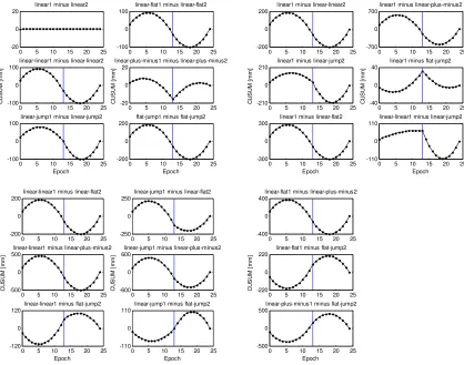
Figure 3: CUSUM simulation results using baseline lengths as input.
If the technique is modified in order to use first differences (between successive epochs) as input rather than the original baseline lengths, any sudden change in slope of the CUSUM (here between epochs 13 and 14) can easily be detected (Figure 4). All cases investigated exhibit a clear peak or jump in the CUSUM chart corresponding to the introduced change, with the obvious exception of combining two uninterrupted linear trends which results in a flat straight line.
The effect of a change in trend occurring in both baselines of the pair but in different epochs (say, two epochs apart) was also investigated and resulted in the peaks or jumps being disguised to an extent. In some cases both changes could be detected rather clearly, while in others the second change point was completely masked by the first and not detectable.
0 5 10 15 20 25 -20
0
20 linear1 minus linear2
0 5 10 15 20 25
-20 0
20linear-linear1 minus linear-linear2
C U S U M [ m m ]
0 5 10 15 20 25
-25 0
25linear-jump1 minus linear-jump2
Epoch
0 5 10 15 20 25
-20 0
20 linear-flat1 minus linear-flat2
0 5 10 15 20 25
-30 0 30
linear-plus-minus1 minus linear-plus-minus2
C U S U M [ m m ]
0 5 10 15 20 25
-10 0
10 flat-jump1 minus flat-jump2
Epoch
0 5 10 15 20 25
-30 0
30 linear1 minus linear-linear2
0 5 10 15 20 25
-60 0
60 linear1 minus linear-jump2
C U S U M [ m m ]
0 5 10 15 20 25
-50 0
50 linear1 minus linear-flat2
Epoch
0 5 10 15 20 25
-90 0
90linear1 minus linear-plus-minus2
0 5 10 15 20 25
-15 0
15 linear1 minus flat-jump2
C U S U M [ m m ]
0 5 10 15 20 25
-50 0
50linear-linear1 minus linear-jump2
Epoch
0 5 10 15 20 25
-30 0
30linear-linear1 minus linear-flat2
0 5 10 15 20 25
-80 0 80
linear-linear1 minus linear-plus-minus2
C U S U M [ m m ]
0 5 10 15 20 25
-30 0
30linear-linear1 minus flat-jump2
Epoch
0 5 10 15 20 25
-50 0
50linear-jump1 minus linear-flat2
0 5 10 15 20 25
-100 0
100linear-jump1 minus linear-plus-minus2
C U S U M [ m m ]
0 5 10 15 20 25
-30 0
30linear-jump1 minus flat-jump2
Epoch
0 5 10 15 20 25
-70 0
70linear-flat1 minus linear-plus-minus2
0 5 10 15 20 25
-50 0
50 linear-flat1 minus flat-jump2
C U S U M [ m m ]
0 5 10 15 20 25
-80 0
80linear-plus-minus1 minus flat-jump2
[image:6.595.79.502.71.399.2]Epoch
Figure 4: CUSUM simulation results using first differences as input.
5. Case study: Ice shelf rift propagation
GPS data collected in a network deployed over three weeks during the 2004/05 Antarctic summer period in order to monitor the propagation of an active ice shelf rift system on the Amery Ice Shelf, East Antarctica were used to validate the findings from the simulation above. As opposed to crevasses, rifts are defined as fractures that penetrate through the entire ice shelf thickness (~400 m in this case). Located at the front of the Amery Ice Shelf, this active rift system, known as the Loose Tooth, encompasses an area of about 30 km by 30 km that will likely break off and produce a relatively large iceberg in the near future. It consists of two longitudinal-to-flow rifts (denoted L1 and L2) which originated around 20 years ago and two transverse-to-flow rifts (denoted T1 and T2) which formed in 1995 (Figure 5). Evidence has been presented that rift propagation occurs in episodic bursts and is primarily driven by the internal glaciological stress of the ice shelf, rather than initiated by winds or ocean tides (Bassis et al. 2005, Janssen et al. 2009).
Figure 5: (a) Amery Ice Shelf (image courtesy of Australian Antarctic Data Centre), (b) Landsat-7 ETM+ image of the Loose Tooth rift system acquired on 2 March 2003, and (c) location of GPS stations around the tip of T2
overlaid on a Landsat-7 image acquired on 9 January 2005.
Part of this GPS network, situated around the tip of the T2 rift, is depicted in Figure 5c, showing the 8 sites used in this study. The regular pattern of black lines visible represents data gaps caused by the failure of the SLC
[image:6.595.91.498.583.704.2](Scan Line Corrector) module in the ETM+ sensor on the Landsat-7 satellite, which occurred on 31 May 2003. The SLC function was necessary to compensate for the forward motion of the satellite during data acquisition – its failure causes individual image scans to overlap and results in the loss of about 22% of the data in each image (USGS 2009).
The dual-frequency GPS receivers, powered by batteries and solar panels, operated at a sampling rate of 30 seconds, and daily (24-hr) sessions were processed to generate baseline length time series, using IGS precise ephemerides and full antenna phase centre variation models. The Saastamoinen model was applied to account for the tropospheric delay, while an ionosphere model was computed from the reference station data of each baseline.
Figure 6 shows the baseline length time series obtained, relative to the first day of data collection. On first inspection, typical deformational behaviour can be recognised including relatively uniform linear trends, increasing linear trends, and linear trends converting to a constant or decreasing baseline length. However, in order to detect subtle baseline length changes in this dynamic environment, a more detailed analysis is required.
0 5 10 15 20 25
419.5 420
420.5 T2S5-T2N1
0 5 10 15 20 25
1033.5 1034.5 1035.5 T2S5-T2S6 B as el in e Le ng th [m ]
0 5 10 15 20 25
1101.5 1102
1102.5 T2N6-T2N1
Days since 18 Dec 2004
0 5 10 15 20 25
525 525.5
526 T2N5-T2S1
0 5 10 15 20 25
1016.5 1017 1017.5 T2S5-T2S2 B as el in e Le ng th [m ]
0 5 10 15 20 25
1202 1202.5
1203 T2N2-T2N1
Days since 18 Dec 2004
0 5 10 15 20 25
1026.5 1027
1027.5 T2N5-T2N6
0 5 10 15 20 25
1088 1088.5 1089 T2S1-T2S6 B as el in e Le ng th [ m ]
0 5 10 15 20 25
1133.5 1134
1134.5 T2N5-T2N2
0 5 10 15 20 25
1108.5 1109 1109.5 T2S1-T2S2 B as el in e Le ng th [ m ]
[image:7.595.85.504.245.405.2]Days since 18 Dec 2004 Days since 18 Dec 2004
Figure 6: Baseline length time series in the Loose Tooth GPS network.
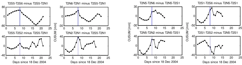
Several baseline pairs of the Loose Tooth GPS network were analysed using the CUSUM technique described above. The baseline pairs were chosen to include one across-rift tip baseline located normal to the rift (either T2S5-T2N1 or T2N5-T2S1) and one baseline aligned approximately parallel to the propagating rift (see Figure 5c). A known jump of ~1 cm in baseline length across the rift tip on day 9, inferred from seismic data collected at the sites and attributed to the episodic nature of rift propagation (Bassis et al. 2007), can be reliably detected as a peak on day 8 in most pairs (Figure 7). As evident in the rightmost panels of the figure, the jump is masked by other activity or increased noise present in some baseline pairs. This example emphasises the importance of analysing a number of baseline pairs.
0 5 10 15 20 25
-80 0
80 T2S5-T2S6 minus T2S5-T2N1
0 5 10 15 20 25
-40 0
40 T2S5-T2S2 minus T2S5-T2N1
C U S U M [ m m ]
0 5 10 15 20 25
-30 0
30 T2N6-T2N1 minus T2S5-T2N1
0 5 10 15 20 25
-40 0
40 T2N2-T2N1 minus T2S5-T2N1
C U S U M [ m m ]
Days since 18 Dec 2004 Days since 18 Dec 2004
0 5 10 15 20 25
-30 0
30 T2N5-T2N6 minus T2N5-T2S1
0 5 10 15 20 25
-40 0
40 T2N5-T2N2 minus T2N5-T2S1
C U S U M [ m m ]
0 5 10 15 20 25
-50 0
50 T2S1-T2S6 minus T2N5-T2S1
0 5 10 15 20 25
-40 0
40 T2S1-T2S2 minus T2N5-T2S1
C U S U M [ m m ]
Days since 18 Dec 2004 Days since 18 Dec 2004
[image:7.595.90.502.541.652.2]evident due to the limited number of baselines available. In order for a jump to be reliably determined, it is required to be present in multiple baseline pairs.
6. Concluding remarks
Analysis of a GPS network using a cumulative sum (CUSUM) approach, obtained by differencing a pair of residual baseline time series situated approximately normal and parallel to the direction of expected deformation, is found to be an effective method to detect small baseline length changes. Simulation shows that using first differences (between successive epochs) as input, rather than the original baseline lengths, produces clear peaks or jumps in the CUSUM charts when a sudden change in baseline length occurs. This is confirmed by the results obtained from GPS data collected in close proximity to a propagating ice shelf rift, reliably identifying a jump in the across-rift tip baseline length time series that can be attributed to rift opening. This technique is well suited for a variety of deformation monitoring applications and can, with a few modifications, be used to detect baseline length changes in real time.
Acknowledgements
GPS data collection was supported by the Australian Government Antarctic Division through an Australian Antarctic Science grant (#2338) to Prof. Richard Coleman who is gratefully acknowledged for providing these data and invaluable advice during the course of this study. Work at the University of Tasmania was supported by an IRGS grant (J0015638) to the author.
References
Aspinall, W. P., Carniel, R., Jaquet, O., Woo, G., and Hincks, T., Using hidden multi-state Markov models with multi-parameter volcanic data to provide empirical evidence for alert level decision-support, Journal of Volcanology and Geothermal Research 153:1-2 (2006), 112–124.
Basseville, M. and Nikiforov, I. V., Detection of abrupt changes: Theory and applications, Prentice Hall, Eaglewood Cliffs, USA, 1993.
Bassis, J. N., Coleman, R., Fricker, H. A., and Minster, J. B., Episodic propagation of a rift on the Amery Ice Shelf, East Antarctica, Geophysical Research Letters 32:2 (2005), L06502, doi:10.1029/2004GL022048. Bassis, J. N., Fricker, H. A., Coleman, R., Bock, Y., Behrens, J., Darnell, D., Okal, M., and Minster, J. B.,
Seismicity and deformation associated with ice-shelf rift propagation, Journal of Glaciology 53:183 (2007), 523–536.
Hinkley, D. V., Inference about the change point in a sequence of random variables, Biometrika 57:1 (1970), 1– 17.
Hinkley, D. V., Inference about the change point from cumulative sum-tests, Biometrika 58:3 (1971), 509–523. Iz, H. B., Differencing reveals hidden changes in baseline length time-series, Journal of Geodesy 80:5 (2006),
259–269.
Janssen, V., Coleman, R., and Bassis, J. N., GPS-derived strain rates on an active ice shelf rift, Survey Review 41:311 (2009), 14–25.
Lee, H. K., Wang, J., and Rizos, C., Effective cycle slip detection and identification for high precision GPS/INS integrated systems, Journal of Navigation 56:3 (2003), 475–486.
Lorden, G., Procedures for reacting to a change in distribution, Annals of Mathematical Statistics 42:6 (1971), 1897–1908.
Lucas, J. M. and Crosier, R. B., Fast initial response for CUSUM quality-control schemes: Give your CUSUM a head start, Technometrics 24:3 (1982), 199–205.
Mertikas, S. P., Automatic and online detection of small but persistent shifts in GPS station coordinates by statistical process control, GPS Solutions 5:1 (2001), 39–50.
Mertikas, S. P. and Damianidis, K. I., Monitoring the quality of GPS station coordinates in real time, GPS Solutions 11:2 (2007), 119–128.
Mertikas, S. P. and Rizos, C., Online detection of abrupt changes in the carrier phase measurement of GPS, Journal of Geodesy 71:8 (1997), 469–482.
Mohanty, W. K., Routray, A., and Nath, S. K., A new strategy for phase detection in seismic signals using an adaptive Markov amplitude model, Current Science 93:1 (2007), 54–60.
Moustakides, G. V., Optimality of the CUSUM procedure in continuous time, Annals of Statistics 32:1 (2004), 302–315.
Ogaja, C., A software implementation of multi-sensor data analysis and GPS integrity assessment for real-time monitoring applications, in: Kahmen, H., Niemeier, W., and Retscher, G., editors, Proceedings of the 2nd Symposium on Geodesy for Geotechnical and Structural Engineering, Berlin, May 21–24, 2002, 27–37, 2002.
Page, E. S., Continuous inspection schemes, Biometrika 41:1-2 (1954), 100–115.
Page, E. S., On problems in which a change in a parameter occurs at an unknown point, Biometrika 44:1-2 (1957), 248–252.
USGS, SLC-off products: Background, http://landsat.usgs.gov/products_slcoffbackground.php (accessed Mar 8, 2009).
Van Dobben de Bruyn, C. S., Cumulative sum tests: Theory and practice, Griffin, London, 1968.
Xie, G., Pullen, S., Luo, M., and Enge, P., Detecting ionospheric gradients with the cumulative sum (CUSUM) method, in: Proceedings of the 21st International Communications Satellite Systems Conference, Yokohama, April 16–19, 2003, paper AIAA2003-2415, 2003.
Author Posting. © Walter de Gruyter GmbH & Co. KG, 2009.