A Constructive Approach Towards Formalizing
Relativization Using Combinatory Logic
MSc Thesis
(Afstudeerscriptie)
written by Marlou M. Gijzen
(born May 9th, 1994 in Haarlem, The Netherlands)
under the supervision of Dr Benno van den BergandDr Leen Torenvliet, and submitted to the Board of Examiners in partial fulfillment of the requirements for
the degree of
MSc in Logic
at theUniversiteit van Amsterdam.
Date of the public defense: Members of the Thesis Committee:
September 12, 2018 Dr Benno van den Berg
Dr Ronald de Haan Frederik Lauridsen MSc Dr Floris Roelofsen (Chair) Dr Leen Torenvliet
Abstract
We present a formal system, ACT, that is used to express the time-complexity of computing functions. Every proof that can be made within the system relativizes. The system uses combinatory logic instead of Turing machines. We do show that it is invariant with respect to Turing machines.
Contents
1 Introduction 1
2 Preliminaries 2
2.1 Basic notions from complexity theory . . . 2
2.1.1 Some complexity classes . . . 3
2.1.2 Oracle machines . . . 3
2.1.3 Relativization and diagonalization . . . 4
2.2 Heyting arithmetic . . . 5
3 Absolute Complexity Theory 6 3.1 The formal systemACT . . . 6
3.2 Relativized worlds . . . 8
4 Conservativity overHA 9 4.1 Coding sets and pairs . . . 10
4.2 Defining the mapping . . . 10
4.3 Conservativity ofACT . . . 11
5 Functions and Lists 13 5.1 The length of a term . . . 13
5.2 Lambda abstractions . . . 13
5.2.1 Complexity of rewriting lambda abstractions . . . 14
5.3 A fixpoint combinator . . . 15
5.4 Arithmetical operations . . . 15
5.4.1 Addition . . . 15
5.4.2 Subtraction . . . 16
5.4.3 Multiplication . . . 17
5.4.4 Division . . . 17
5.4.5 Exponentiation . . . 18
5.4.6 Equality . . . 18
5.5 Lists . . . 19
5.5.1 Lists of natural numbers . . . 19
5.5.2 Operations on lists . . . 20
6 Invariance with respect to Turing Machines 21 6.1 A Turing machine that rewrites terms . . . 21
6.1.1 Encoding terms in binary . . . 21
6.2 A term that simulates Turing machines . . . 25
7 Complexity Results 27 7.1 Universal computation . . . 27
7.2 Enumerating the terms . . . 28
7.3 Complexity classes . . . 29
7.4 Time Hierarchy Theorem . . . 30
7.5 P vsN P is independent fromACT+U . . . 31
7.5.1 Relativized world whereP =N P . . . 31
7.5.2 Realizability with truth . . . 32
7.5.3 Relativized world whereP 6=N P . . . 33
7.5.4 Independence result . . . 34
8 Conclusion 36 9 Acknowledgements 38 10 Bibliography 39 11 Appendix 40 11.1 Proofs of Chapter 5 . . . 40
1 Introduction
In this work, we present a system that can be used to express the time-complexity of computations. Furthermore, every proof in the systemrelativizes.
The notion of relativization plays a mayor role in computational complexity. We say that a proof relativizes when it also holds relative to any oracle. Oracle machines are used to define Turing reductions. They have also been used to obtain a series of results that tell us which proof-techniques we can and cannot use to solve certain problems. We know for example that we need non-relativizing proof-techniques to solve thePvs NP problem.
However, it has never been proven that a proof-technique does not relativize, even though that has been said about, for example, arithmetization.
With this system we formalize the notion of relativization. The axiomatic system is called Absolute complexity theory, ACT, and it is an extension of Heyting arithmetic, HA. It uses combinatory logic as a model for computation. The length of the reduction serves as a benchmark for measuring the time-complexity of solving specific problems. We expect that this system could be used to gain insight in non-relativizing proof-techniques. This information is necessary in order to obtain certainty about the use-fulness of proof-methods for tackling specific problems. We also hope to be able to obtain independence of the Pvs NP problem from general intu¨ıtionistic logics with future work.
In Chapter 2 we outline some preliminary notions. In the following chapter the systemACTis presented.
Chapter 4 treats the conservativity of ACT over HA. In the next chapter we give several terms that compute functions such as addition and multiplication, and we prove the complexity of those computations.
We do not use Turing machines as a model for computation, in contrast to standard computational complexity. However, in Chapter 6 we do show that the system is invariant with respect to Turing machines: both models can simulate each other with only a polynomially-bounded overhead in time.
2 Preliminaries
The formal system that will be presented in Chapter 3 can be used to describe the time-complexity of computations. It is based upon Heyting arithmetic. When we mention areduction we mean a rewriting-step from one term into another. A term in
normal form cannot be reduced to any other term.
In this chapter we will outline some notions from complexity theory that will be used for the formal system, as well as a description of Heyting arithmetic.
2.1 Basic notions from complexity theory
In computational complexity theory problems are categorized according to their diffi-culty. We try to measure the difficulty of problems by considering the amount of some resource that a Turing machine needs to solve a problem.
Definition 2.1.1 ([3, Sec. 1.2]). A Turing machine is described by a tuple (Γ, Q, δ):
• Γ is a finite set of tape symbols, the alphabet.
• Q is a finite set of states.
• δis a transition function: Q×Γ→Q×Γ× {L, R, S}.
It has a one-way infinite read/write tape, a head that it uses for reading and writing on the cells of the tape and a register that holds the state of the machine. A single
computation step is described by one application of the transition function: it reads a symbol in a specific state, and then writes down a symbol on that location, gets into some state and the head moves to the left, right or stays on that location.
A (regular) Turing machine works in adeterministic manner. We can also consider machines that work nondeterministically:
Definition 2.1.2 ([3, Sec. 2.1.2]). A nondeterministic Turing machine is a Turing machine with two transition functions. At each step, the machine chooses which of its transition functions it will apply. When dealing with 0/1-valued functions, we say that a nondeterministic machine accepts an input when one of its possible computational paths accepts (or outputs 1).
A Turing machine usually works with binary strings, and it thus computes functions
f :{0,1}∗→ {0,1}∗. We will consider the amount of time needed for computations.
input, we will refer to functions T :N→Nto describe the computation times. T(n)
gives the number of steps that a machine needs in the worst case for a computation on an input of sizen.
2.1.1 Some complexity classes
In standard computational complexity we usually consider the complexity of 0/1-valued functions or decision problems - i.e., f :{0,1}∗→ {0,1}.
The exact number of steps that are needed for a computation are not important, we are only interested in the biggest growing term of the functionT(n). We thus use the
Big-Oh notation:
Definition 2.1.3. Forf, g : N→ N, f =O(g) when there exists a constant c and some n0∈Nsuch thatf(n)≤c·g(n) for alln≥n0.
In this paper we will refer to three different complexity classes:
Definition 2.1.4 ([7]). The classPis the class of decision problems for which there exists a Turing machine that computes the problem and runs in timeO(p(n)) for some polynomial p.
Definition 2.1.5 ([7]). The classEXPis the class of decision problems solvable by a Turing machine in timeO(2p(n)) for a polynomial p.
Definition 2.1.6 ([7]). The class NP consists of problems solvable in polynomial-time by a nondeterministic Turing machine. We say that the machine accepts when at least one computation path accepts, and it rejects when all computation paths do so.
Equivalently, a decision problem f is inNP when there are polynomialsp and q
such that there exists a Turing machine M that runs in timeO(p(n)) and for every
x∈ {0,1}∗,
f(x) = 1⇔ ∃u∈ {0,1}q(n)s.t. M accepts on input (x, u)
2.1.2 Oracle machines
In addition to the classical notion of a Turing machine, we will also talk about Turing machines that have black-box access to some function:
Definition 2.1.7 ([10, p. 43]). Anoracle Turing machine is a Turing machine with access to some oracle O. The machine has an extra one-way read/write tape, the oracle tape, and a corresponding head. The oracleOrepresents some functionf. The machine also has two additional states: sq, the query state, andsa, the answer state.
When the machine writes an input x on the oracle tape, and when it gets into the statesq, in one step the contents of the oracle tape are replaced by the outputf(x),
We will refer to computations performed by such machines with oracle access to an oracle O as computations relative to O. We can also consider complexity classes relative to oracles. The class PO denotes the class of problems solvable in polynomial
time by an oracle Turing machine with access to O.
In standard computational complexity the oracles that are used are generally also decision problems (or sets). We can use any function as an oracle, but if a machine runs within a specific time-bound, then this puts a limit on the number of bits that the machine can read from the output of the oracle.
2.1.3 Relativization and diagonalization
We call proof-techniques in complexity theory relativizing when the result also holds relative to any oracle. For example, the Time Hierarchy Theorem [8] is shown using
diagonalization, which is regarded as a relativizing proof-technique. The theorem has as a result thatP6=EXP, so this means that we also have thatPO6=EXPO for any
oracle O.
Cantor was the first to use diagonalization in proofs and it can similarly be used in complexity theory.
For diagonalization in standard computational complexity, we need an enumeration of Turing machines and a way to (efficiently) simulate the machines.
For the enumeration, we use some fixed way of describing the Turing machines as binary strings. How this can be done is described in [3, Sec. 1.4]. We make use of two conventions. Firstly, that we can describe every Turing machine with a binary string and every string represents some Turing machine. Secondly, that there is an infinite number of binary strings that represents one Turing machine.
Generally, we use a universal Turing machine to simulate Turing machines based on their description:
Theorem 2.1.1 ([3, Th. 1.9]). There exists a Turing machine U such that for every two inputs x, α ∈ {0,1}∗, U(x, α) = M
α(x), where Mα denotes the machine
repre-sented by the string α. If Mα halts within T steps on input x, then U halts within
CTlogT steps on inputs xandα(withC a number independent of x).
A typical diagonalization proof then goes as follows. For an input x ∈ {0,1}n,
we run U(x, x) for g(n) steps, where g is some function. We can do this by adding a counter for the number of steps to the machine. If the machine halted by then, output the opposite. We then have a function that no machine that runs within time
O(pg(n)) can compute.
Since in most proofs we could just as well diagonalize against oracle Turing machines, diagonalization is believed to be a relativizing proof-technique.
The notion of relativization gives us insight in the proof techniques that we need to solve certain problems. We know that we need non-relativizing proof techniques to solve the PvsNPproblem, since it hasconflicting relativizations:
Theorem 2.1.2 (Baker, Gill, Solovay, 1975, [5]). There exist oracles A, B such that
2.2 Heyting arithmetic
Heyting arithmetic, HA, is a formal system that describes intu¨ıtionistic first order arithmetic. It uses first-order intu¨ıtionistic predicate logic with equality.
It has a constant 0 (zero), a unary function constantS(the successor), and function symbols for all primitive recursive functions.
We have the axioms from the first-order predicate logic, axioms for all the primitive recursive functions, and the following:
¬S0 = 0
Sx=Sy⇒x=y
A(0)∧ ∀x[A(x)→A(Sx)]⇒ ∀xA(x)
In HA every element is a natural number. We can denote the number n by Sn0,
3 Absolute Complexity Theory
We will introduce a formal system called ACT: Absolute complexity theory. It is based upon the systemTAPP, defined by Troelstra in [12, p. 475]. ACToffers a way to describe the complexity of solving partial functions from Nto N, using combinatory
logic.
We will write
x→ny
when a programxcan be rewritten intoywithntime-steps. In the case of computation relative to an oracle f we writex→f
ny.
3.1 The formal system
ACT
The system uses first order intu¨ıtionistic predicate logic with equality (‘=’). There is a unary predicate N, corresponding to being a natural number:
∀x[N(x)⇔x∈N]
We have a constant 0, the successor functionS, and function symbols for all primitive recursive functions.
We also adopt the following axioms:
H.1 0∈N
H.2 x∈N⇒Sx∈N
H.3 ∀x[¬Sx= 0]
H.4 ∀x,y∈N[Sx=Sy⇒x=y]
H.5 ϕ(0)∧ ∀x∈N[ϕ(x)⇒ϕ(Sx)]⇒ ∀x∈Nϕ(x)
We also add the axioms for the primitive recursive function symbols, only we add the predicateN to the axioms such that the variables range over the natural numbers.
With respect to equality we have the following axioms:
E.1 ∀x[x=x]
E.2 ∀x, y[x=y⇒y=x]
E.3 ∀x, y, z[x=y∧y=z⇒x=z] E.4 ∀x, y[x=y∧ϕ(x)⇒ϕ(y)]
Besides this, we have a total binary operation denoted by a dot ‘·’, which stands for application of terms. We assume left associativity and often leave out the ‘·’: when we write xyz, we mean (x·y)·z.
We have a several combinators: k,s,p,p0,p1,succ,predandd. Thekandsare well-known from combinatory logic. Thepis used for paring andp0andp1for projec-tions. We havesuccandpredas successor and predecessor combinators. Finally, the d-combinator represents an if-then-else-construct. We thus have the following basic axioms for the combinators:
B.1 ∀x, y[kxy→1x]
B.2 ∀x, y, z[sxyz→1xz(yz)] B.3 ∀x, y[p0(pxy)→1x] B.4 ∀x, y[p1(pxy)→1y] B.5 ∀x, y[p(p0x)(p1x)→1x]
B.6 ∀x[succx→1Sx] B.7 ∀x[predSx→1x] B.8 pred0→10
B.9 ∀x, y, z[d(Sx)yz→1y] B.10 ∀y, z[d0yz→1z]
We have the following axioms that we use to rewrite terms: A.1 ∀x, y, z[x→zy⇒z∈N]
A.2 ∀x, y, n[x→n y⇒ ∀m≥n[x→my]]
A.3 ∀x, y, z, n, m[x→n y∧y→mz⇒x→n+mz]
A.4 ∀x, y, z, n[x→ny⇒x·z→ny·z]
A.5 ∀x, y, z, n[x→ny⇒z·x→nz·y]
A.6 ∀x, n, y1, y2[x→n y1∧x→ny2⇒ ∃z, m[y1→mz∧y2→mz]]
A.7 ∀x[N(x)⇒ ∀y, n[x→n y⇒y=x]]
Axiom A.1 ensure that the ternary predicate→has a natural number to denote the number of steps for rewriting. Axiom A.2 says that if we can deducey fromxwithin
n steps, then it is also possible for any number of steps bigger than n. Axiom A.3 enables us to combine different reductions. The axioms A.4 and A.5 are needed for the ability to rewrite certain parts of a term at a time. Axiom A.6 expresses that the order of the reductions has no influence on the final result (as in the Church-Rosser Theorem). Axiom A.7 states that natural numbers are in normal form.
We also use the following abbreviations:
x→y:=∃n[x→ny]
x=. y:=∀n∈N∃z, m∈N[x·n→mz∧y·n→mz]
3.2 Relativized worlds
We will define another axiomatic system, extending ACT. For any total computable functionf :N→N, that is definable inACT, we have a systemACTf, wheref can be used as an oracle for the computations.
Since f is computable, we thus have by assumption that there exists an term that computes the function and we will fix a canonically chosen termtf.
Instead of using → as a symbol for the ternary predicate, we will now use →f to
denote computations relative tof.
The axioms of ACTf are the same as those of ACT, except we use the symbol →f
everywhere. We also add one combinator and a corresponding axiom. Letf(x) denote the output off on inputx. Then:
B.11 ∀x∈N[ofx→ f
1S
f(x)0]
We thus have that ACT` ∀x∈N∃m∈N[tfx→mf(x)].
We have that every query to the oracle can be replaced by actually computing f, and the other way around. Thus, for any term tf that computesf, and for anyxin
the domain off, there exists an msuch thattf·x→mf f(x)⇔of·x→ f
1 f(x). Since all the other axioms of ACTf are the same axioms as in ACT, we have the following:
Corollary 3.2.1. For allϕ,ACT`ϕ⇒ACTf `ϕ
4 Conservativity over
HA
We would like to show that the systems ACT and ACTf for any f are conservative overHA.
Definition 4.0.1. A theoryT0 is a conservative extension of a theory T iff
T0`ϕ⇒T `ϕ
for all formulas ϕin the language of T.
If we achieve this, we can conclude thatACT is consistent, given the consistency of HA. We also know thatACTsays as much about the natural numbers as HAdoes.
However, there is one problem. InHAall free variables are natural numbers and we only quantify over natural numbers. This is not the case in ACT. Since we are only interested in formulas that are expressible in the language ofHA, we will instead show the following:
ACT`ϕN⇒HA`ϕ
for all formulas ϕin the language of HA. The mapping·Ntakes formulas to similar formulas, but the free variables are natural numbers and quantifiers range over natural numbers.
This means that we will not achieve actual conservativity over HA. However, we will be able to conclude the things that we wanted to know about ACT (consistency and expressibility with respect to natural numbers).
We define·N formally as follows: Definition 4.0.2.
φ(x1, . . . , xn)N:=N(x1)∧. . .∧N(xn)∧φ(x1, . . . , xn) for atomic formulasφ
(φ∗ψ)N:=φN∗ψNfor∗ ∈ {∨,∧,→} (∀xφ)N:=∀x∈
NφN
(∃xφ)N:=∃x∈
NφN
In the rest of this chapter we will focus on a mapping J·K from formulas of the language ofACTto formulas of the language ofHA, which serves as a way to interpret ACT inHA. We will then show
After proving that
HA`(JϕN
K⇔ϕ)
for formulasϕin the language ofHA, we can conclude that ACT`ϕN⇒HA`ϕ
for all formulas ϕin the language ofHA. This is also how Troelstra suggests showing that TAPPis conservative overHA[12, p. 489]. The case forACTf is similar.
For the mappingJ·K, we will focus us on RE(ω), recursively enumerable subsets of
N. In HAwe have function symbols for the primitive recursive functions, so we can
describe all elements ofRE(ω) (the range of a primitive recursive function is recursively enumerable). Since Kleene’s T-predicate is also primitive recursive, we can describe all elements of RE(ω) using only a single primitive recursive function symbol. This allows us to quantify over the elements ofRE(ω).
Kleene’s T-predicate relies on a G¨odel numbering that assigns functions to natural numbers. We then have that T(nx, m, z) is true when z encodes a valid and halting
computation of the computable function with indexnxon inputm. A setX inRE(ω)
can be described as {m| ∃z(T(nx, m, z))} or{m|ϕ(nx, m)}.
4.1 Coding sets and pairs
First, we have to fix a coding p for pairs. We will choose the well-known function
p(x, y) =12(x+y)(x+y+ 1) +y, but we will write (x, y) as an abbreviation. We will also use a coding for finite sets:
{k0, . . . , kp}:=Ppi=02ki
{∅}:= 0
Note that 2n codes {n}.
4.2 Defining the mapping
As in [12, p. 484], we can define a total application operation·by:
X·Y :={z| ∃y ⊂Y((y, z)∈X)}. When we sayy ⊂Y then we mean that the set that is coded byy is a subset of Y. We letJX·YK:=JXK·JYK.
The application of two recursively enumerable sets is again recursively enumerable. This can be seen as follows: for an inputz, we enumerate the elements of bothY and
X step-by-step. With every new element ofY in the enumeration, for all pairs (y, z) in the enumeration of X, we check whether y encodes a subset of the already listed elements of Y. If yes, we acceptz.
Variables are mapped to themselves. For the constants that are also in the language ofHAwe do the following:
J0K:={0} JS(n)K:={n+ 1}
Also as defined in [12] we have the following definitions for the combinators:
JkK:={(x,(y, z))|z∈x} JsK:={(x,(y,(z, w)))|z
0⊂z((z0,(u, w))∈x)∧ ∀u0∈u∃z0⊂z((z0, u0)∈y)}
JsuccK:={(2
n, n+ 1)|n∈
N}
JpredK:={(2
n, n−1)|n∈
N}
JpK:={(2
n,(0,2n))|n∈
N} ∪ {(0,(2m,2m+ 1))|m∈N}
Jp0K:={(2
2n, n)|n∈
N}
Jp1K:={(2
2n+1, n)|n∈
N}
JdK:={(2
n
,(x,(y, z)))|n= 0∧z∈y∨ ¬n= 0∧z∈x}
We also have the following predicates:
JX =YK:=JXK=JYK
JX →nYK:=JXK=JYK∧JN(n)K JN(X)K:=∃n[2
n =X]
For∨,∧,⇒,∀xand∃ywe letJ·Kact as a homomorphism.
4.3 Conservativity of
ACT
Lemma 4.3.1. For all formulasϕ,ACT`ϕ⇒HA`JϕK
Proof.We prove this by showing that all axioms ofACT(that are not already inHA) hold inHAunder the mapping.
From the basic axioms, we will show that (JkK·X)·Y =X, and leave the verification of the other basic axioms to the reader.
(JkK·X)·Y ={a| ∃x⊂X((x, a)∈JkK)} ·Y
={b| ∃y⊂Y((y, b)∈ {a| ∃x⊂X((x, a)∈JkK)})}
={b| ∃y⊂Y ∧ ∃x⊂X((x,(y, b))∈JkK)}
=X
Now for the other axioms:
A.1 ∀x, y, zJx→zy⇒N(z)K=∀X, Y, Z[X =Y ∧ ∃n(2
n=Z)⇒ ∃n(2n=Z)]
Which always holds.
A.2 ∀x, y, nJx→n y⇒ ∀m≥n[x→my]K
=∀X, Y, n[X =Y ∧ ∃z(2z=n)⇒J∀m≤nK[X =Y ∧ ∃z(2
z=m)]]
A.3 ∀x, y, z, n, mJx→n y∧y →m z ⇒ x→n+m zK= ∀X, Y, Z[X = Y ∧Y = Z ⇒
X=Z]
This is obviously true. The last two axioms also follow quite easily: A.4 ∀x, y, z, nJx→ny⇒x·z→ny·zK=∀X, Y, Z[X=Y ⇒X·Z=Y ·Z]
Assume that X = Y. Then:
X·Z={a| ∃z⊂Z((z, a)∈X)}
={a| ∃z⊂Z((z, a)∈Y)}
=Y ·Z
A.5 ∀x, y, z, nJx→ny⇒z·x→nz·yK=∀X, Y, Z[X=Y ⇒Z·X=Z·Y]
Assume that X = Y. Then:
Z·X={a| ∃x⊂X((x, a)∈Z)}
={a| ∃y⊂Y((y, a)∈Z)}
=Z·Y
Theorem 4.3.2. ACT`ϕN⇒HA`ϕfor all formulasϕin the language ofHA
Proof. We will show that for formulas ϕ in the language of HA: HA`(ϕ⇔JϕN
K).
Then, with Lemma 4.3.1 the theorem follows.
We will show this by induction on the formulas. First, we consider atomic formulas. We have thatHA`Ja=bKis equal toHA`JaK=JbK, whereaandbcould be of the form 0, S(n) or F(x1, . . . , xn). Looking at the definition of J·Kfor these (functional)
constants, we see thatHA`Ja=bK⇔a=b, since the left side is equality of singletons that are equal toaandb itself.
For most logical connectives,J·Kand·Nact as a homomorphism. The only noticeable
cases are the quantifiers, since then ·Nacts differently.
The axioms concerning the primitive recursive function symbols and the successor symbol were modified inACTsuch that they quantified over natural numbers only. In HA every variable is a natural number, and thus it quantifies solely over the natural numbers. So we can conclude that for allϕ,HA`(ϕ⇔JϕN
K).
Corollary 4.3.1. ACTf ` ϕN ⇒ HA` ϕ for all formulas ϕ in the language of HA
and total recursivef that are definable inACT.
Proof.Lettf be the chosen term that computes the functionf. We let JofK:=JtfK.
InACTwe should have a proof of ∀x∈N∃m∈N[tf ·x→mf(x)]. Then with Lemma
5 Functions and Lists
In this chapter, we will define several functions and discuss the complexity of solving them. We will also outline how we can use lists inACT. We will restrict our attention to lists of natural numbers and functions fromNtoN. In order to make the definitions
of functions easier, we will explain how we can introduce lambda abstractions such as
λx.t(x).
5.1 The length of a term
Before we can start to work with lists and the complexity of solving lambda abstrac-tions, we will have to define the length of a term. We will avoid terms that contain primitive recursive function symbols. As we will see in Chapter 6, for each primi-tive recursive function there exists a term that computes that function using only the combinators and the binary application symbol.
Definition 5.1.1 (The length of a term).
`(0) = 1 For allx,`(Sx) = 1 +`(x) For all combinatorsc,`(c) = 1
For variablesx,`(x) = 1
`(t1·t2) = 1 +`(t1) +`(t2)
As a result, we have that forn∈N, `(n) =n+ 1.
5.2 Lambda abstractions
We can rewrite terms such that they behave similarly to reducing lambda abstractions: Proposition 5.2.1. For each expression t(x) with a variable x, there exists a term
λx.t(x) such that for each term b in the language of ACT, ACT `λx.t(x)·b =t(b), where t(b)is a term in the language ofACT withb in place of the variablex.
For example, the termλx.d(x)(1)(0) will return ‘1’ when abapplied to it is a natural number bigger than zero, and it will return ‘0’ whenb= 0.
Proof of Proposition 5.2.1.We will builtλx.t(x) with induction on the structure of
t(x), similarly to for example [12, Prop. 9.3.5]. Ift(x) isxitself, thenλx.t(x) =skk. If
t(x) is a variable or constantcdifferent fromx, thenλx.t(x) =kc. Ift=t1(x)·t2(x), thenλx.t(x) =s(λx.t1(x))(λx.t2(x)).
5.2.1 Complexity of rewriting lambda abstractions
For all termsλx.t(x) andb, we can calculate the time it takes to rewriteλx.t(x)·binto
t(b). This does not take into account the time to rewrite t(b) into a term in normal form. We will eventually prove the following theorem:
Theorem 5.2.1. For allt(x1, . . . , xn)there exists a k∈Nsuch that for allb1, . . . , bn
ACT`λx1, . . . xn.t(x1, . . . , xn)·b1·. . .·bn→k t(b1, . . . , bn).
In order to make general statements about the complexity of rewriting terms with a lambda abstraction, we have to say something about the length of those abstractions. We will prove the following lemma:
Lemma 5.2.2. `(λx.t(x))≤5`(t(x))
Proof.We will show this by induction on the structure oft(x). Whent(x) isxitself, then `(λx.t(x)) = 5. When t(x) is a variable or constant c different from x, then
`(λx.t(x)) = 2 +`(c).
Ift=t1(x)·t2(x), then`(λx.t(x))≤3 +`(λx.t1(x)) +`(λx.t2(x)) I.H.
≤ 3 + 5`(t1(x)) + 5`(t2(x))≤5 + 5`(t1(x)) + 5`(t2(x)) = 5(1 +`(t1(x) +`(t2(x))) = 5`(t(x)).
We can now say something about the complexity of rewriting lambda expressions: Lemma 5.2.3. For allb,λx.t(x)·b→2`(t(x)) t(b)
So to continue with our previous example, we will calculate thensuch that
λx.d(x)(1)(0)·b→nd(b)(1)(0).
For all lambda abstractions, thisnis independent ofb.
Proof.We will show this by induction on the complexity oft(x).
If t(x) is is xitself, thenλx.t(x)·b =skkb→2 b. Whent(x) is a constantc, then
λx.t(x)·b=kcb→1c.
Now for the induction step, assume that t(x) = t1(x)·t2(x). Then `(t(x)) = 1 +
λx.t(x)·b=s(λx.t1(x))(λx.t2(x))b
→1λx.t1(x)·b(λx.t2(x)·b) (I.H.)→2`(t1(x))t1(b)(λx.t2(x)·b)
(I.H.)→2`(t2(x))t1(b)(t2(b))
=t(a)
And 1 + 2`(t1(x)) + 2`(t2(x))≤2`(t(x)).
We can now turn to the proof of the main theorem:
Proof of Theorem 5.2.1. We will show that the theorem holds with
k= 2`(t(x1, . . . , xn))× n−1 X
i=0 5i.
We will use induction. Lemma 5.2.3 shows us that the statement is true for n= 1. Now assume that it holds fornand let|x|= (x1, . . . , xn+1).
Then by the induction hypothesis, we need 2`(λxn+1t(x1, . . . , xn+1))×P
n−1
i=0 5
isteps
to rewriteλx1. . . . λxn+1·t(|x|)·b1·. . .·bn+1 intoλxn+1.t(b1, . . . , bn, xn+1)·bn+1. Then, by Lemma 5.2.3, we need 2×`(t(|x|)) steps to rewrite it intot(b1, . . . , bn+1). Then, with Lemma 5.2.2, we have that the total number of steps is
2`(λxn+1.t(|x|))×P
n−1
i=0 5
i+ 2`(t(|x|)) = 2×5×`(t(|x|))×Pn−1
i=0 5
i+ 2`(t(|x|))
= 2`(t(|x|))×Pn
i=05
i.
5.3 A fixpoint combinator
In order to reproduce recursion, we will use a fixpoint combinator. There exists a fixpoint combinatorF for theSK-calculus:
Definition 5.3.1 ([13, p. 6]). F =ssk(s(k(ss(s(ssk))))k) We have the following:
Proposition 5.3.1. There exists aksuch that for all x,ACT`F x→kx(F x):
Proof.Trivial.
5.4 Arithmetical operations
5.4.1 Addition
Definition 5.4.1.
plus0:=λx.λy.λz.d(z)(succ(x·y·(predz)))(y) plus:=F·plus0
As a recursive algorithm it would look like this:
plus (n ,m) : I f m = 0 ,
o u t p u t n
e l s e
−> p l u s ( n , m−1) + 1
Proposition 5.4.1. ACT` ∃c∀n, m∈N[plus·n·m→c(m+1)n+m]. Proof.We will show this with induction. Assume that m= 0. Then,
plus·n·0 =F·plus0·n·0 (Prop. 5.3.1)→kplus0·plus·n·0
(Th. 5.2.1)→c0 d(0)(succ(plus·n·(pred0)))(n)
→1n
If we take c=k+c0+ 3 thenplus·n·0→cn+m
Now assume that the statement holds for m.
plus·n·m+ 1 =F·plus0·n·m+ 1
→kplus0·plus·n·m+ 1
→c0 d(m+ 1)(succ(plus·n·(predm+ 1)))(n)
→1succ(plus·n·(predm+ 1))
→1succ(plus·n·m) (I.H.)→c(m+1)succ(n+m)
→1n+m+ 1
We have thatk+c0+ 1 + 1 +c(m+ 1) + 1 =c(m+ 2).
5.4.2 Subtraction
Definition 5.4.2.
min0:=λx.λy.λz.d(z)(pred(x·y·(predz)))(y) min:=F·min0
As a recursive algorithm it would be written like this (but inACT, 0−1 orpred0 gives 0).
min(n ,m) : I f m = 0 , o u t p u t n
e l s e
−> min ( n , m−1) − 1
Proposition 5.4.1. ACT` ∃c∀n, m∈N[min·n·m→c(m+1)n−m].
The proof of this proposition, and the rest of the propositions in this chapter, can be found in the Appendix.
5.4.3 Multiplication
We can perform multiplication of natural numbers with this term: Definition 5.4.3.
times0:=λx.λy.λz.d(z)(d(predz)(plus(x·y·(predz))y)(y))(0) times:=F·times0
times (n ,m) : I f m = 0
o u t p u t 0
e l s e i f m=1
o u t p u t n
e l s e
−> t i m e s ( n , m−1) + n
Proposition 5.4.2. ACT` ∃c∀n, m∈N[times·n·m→c(m+1)(n+2)n×m].
5.4.4 Division
Definition 5.4.4.
div0:=λx.λy.λz.d(predz)(d(min·y·z)(succ·(x·(min·y·z)·z))(1))(y) div:=F·div0
div (n ,m) : I f m> 1
i f n >m
−> div( n−m, m) + 1
e l s e
o u t p u t 1
e l s e
o u t p u t n
Proposition 5.4.3. ACT` ∃c∀n, m∈N[div·n·m→c(m+2)dn med
n me].
5.4.5 Exponentiation
The following terms allow us to compute the exponent of two numbers. Definition 5.4.5.
exp0:=λx.λy.λz.d(z)(times·y·(x·y·(predz)))(1) exp:=F·exp0
exp(n ,m) : I f m=0
−> t i m e s ( n , exp ( n , m−1))
e l s e
o u t p u t 1
Proposition 5.4.4. ACT` ∃c∀n, m∈N[exp·n·m→c(n+2)Pm−1
i=0 (ni+1)n
m].
5.4.6 Equality
The following functions works on two natural numbers. It outputs 1 when they are equal, and 0 when the numbers are unequal.
Definition 5.4.6.
e (n ,m) : i f n > 0
i f m> 0
−> e ( n−1 , m−1)
e l s e
o u t p u t 0
e l s e
i f m> 0 o u t p u t 0
e l s e
o u t p u t 1
Proposition 5.4.5. Let min(x, y) denote the minimum ofxandy. Then,
ACT` ∃c∀n, m∈N[ec(min(n,m)+1)z],
where z= 1 whennand mare equal andz= 0 otherwise.
5.5 Lists
5.5.1 Lists of natural numbers
Lists are constructed by repeated pairing. We need something to represent the empty list. Because our if-then-else combinator d works with natural numbers in the if-statement, it is the most convenient to somehow denote the empty list with natural numbers. We therefore chose to represent the empty list withp00. In order to distin-guish the 0’s in the empty list from the other natural numbers, we will add 1 to every number in the list. A delimited list [a0, a1, . . . , an−1] is then represented by
p(a0+ 1)(p(a1+ 1). . .(p(an−1+ 1)p00). . .).
We will denote the length of a listtbylh(t). In Section 5.5.2 we will give functions for giving the length of a list and obtaining an element at a certain index. We have that `(p00) = 5 and lh(p00) = 0. We also have the following:
Lemma 5.5.1. When t is a list of natural numbers, all smaller than some N, then
`(t)≤(N+ 5)×lh(t) + 5.
Proof.Lettbe a list of natural numbers of lengthm, sot=pn0pn1p· · ·pnm−1p00.
Then `(t) will be equal to 5 plus the number ofp0s int without thep00. Thus,`(t) is equal tolh(t) plus the number of applications, which is 2lh(t) plus the sum of the natural numbers that appear int. So`(t) = 5 + 3lh(t) +Plh(t)−1
i=0 (`(ti) + 1). Since all
natural numbers intare bounded byN, and for ann∈N`(n) =n+ 1, we have that
Plh(t)−1
5.5.2 Operations on lists
We will define functions that give the length of a list, and give an element at a certain index of the list. We will denote elements of a sequence s at index i with si, where
the first element has index 0. The following function will give the length of a list: Definition 5.5.1.
len0:=λx.λy.d(p0y)(succ(x·(p1y)))(0) len:=F·len0
len ( s ) :
I f s h a s a f i r s t e l e m e n t x −> l e n ( t a i l ( s ) ) + 1
e l s e
o u t p u t 0
The functiontail(s) is taken from the programming language Haskell and gives the listswithout the first element. The first element of a list sis given byhead(s).
We can give the complexity of calculating the length of a list of natural numbers, but ACThas no way of checking that some term sis actually such a list.
Proposition 5.5.1. Whensis a sequence of natural numbers of length n, then
ACT` ∃c[len·s→c×n n].
The following function gives an element at a certain index: Definition 5.5.2.
ind0 :=λx.λy.λz.d(z)(x·(p1y)(predz))(p0y) ind:=F·ind0
ind ( s , n ) : I f n=0
o u t p u t head ( s )
e l s e
−> i n d ( t a i l ( s ) , n−1)
Proposition 5.5.2. Whensis a sequence of natural numbers of length n, then
6 Invariance with respect to Turing
Machines
We have to argue that the system ACT acts a reasonable model of computation. A definition of a reasonable model is stated in theInvariance Thesis, from Slot and van Emde Boas [11]:
Invariance Thesis. Reasonable models of computation simulate each other with poly-nomially bounded overhead in time and constant factor overhead in space.
It was already proven that lambda calculus is such a reasonable model with respect to time-bounded computation [1, 2]. In order to prove that this also holds forACT, we will show two things. Firstly, that there is a Turing machine that can rewrite a term using the axioms of ACT with a number of steps that is at most polynomially many more than we would have used in the system itself. Secondly, that for each Turing machine there is a term that will simulate it using at most polynomially many more steps than the machine itself.
There is one issue: the rewriting of terms is not deterministic. We will fix a specific rewriting rule for showing these two results. Namely, we will rewrite the terms using the axiom for the leftmost combinator that can be rewritten.
6.1 A Turing machine that rewrites terms
We will describe a Turing machine that simulates the rewriting of terms inACT. That is, we prove the following theorem:
Theorem 6.1.1. There is a Turing machine that with the binary description of a term
t as an input, outputs z in poly(n`(t)) steps whent→n z using a leftmost
reduction-technique and z is in normal form.
Before we do this, we need to show how we represent terms as binary strings.
6.1.1 Encoding terms in binary
We can uniquely encode terms as binary strings, and give an upper bound to the length of the encoding. This work is inspired by the work of Tromp [13]. We will represent binary strings as a concatenation of the numbers0and1in bold, so014≡[0,1,1,1,1].
Definition 6.1.1.
hki ≡012
hsi ≡013
hpi ≡014
hp0i ≡015
hp1i ≡016
hsucci ≡017
hpredi ≡018
hdi ≡019
Forn∈N,hni ≡01n+10 hx·yi ≡01hxihyi
Each binary sequence encodes a term. For a sequence s, we will denote the cor-responding term with s. Any sequence of zeroes at the end of the encoding can be ignored. So, for all terms tandn∈N,hti=hti0n=t.
We can give the following upper-bound on the length of the encoding:
Lemma 6.1.2. We have that`(hxi)≤82·`(x), so the length of the encoding is linear in the size of the represented term.
Proof.This can be shown with induction. We have that:
`(hni) =`(01n+10)
(Lem. 5.5.1)≤(2 + 5)·(n+ 11) + 5 = 7(n+ 1) + 75 = 7(`(n)) + 75
≤82`(n)
Now assume that the statement holds for xandy. Then:
`(hx·yi) =`(01hxihyi)
=`(01)−5 +`(hxi)−5 +`(hyi) (I.H.)≤11 + 82`(x)−5 + 82`(y)
≤82(1 +`(x) +`(y)) = 82`(x·y)
6.1.2 Simulating the reduction steps
Before we can introduce the algorithm that rewrites the terms, we will need to verify that our terms cannot grow too fast in length, similarly to how invariance for lambda calculus was proven in [1]. We also need an additional definition:
Definition 6.1.2. We say thatxis asubterm of t whenxist itself orxappears in
t by application with other terms.
In order to verify that the terms cannot grow exponentially using a polynomially number of steps, we will show the following:
Lemma 6.1.3. When t →k u, by always applying the axiom for the leftmost
com-binator that can be rewritten, then at every reduction-step, nothing that is dupli-cated contains two identical subterms that appeared by a single-step duplication, so
`(u)≤(k+ 1)`(t).
The proof of this lemma can be found in the Appendix.
We also need to make sure that choosing the subterm that we will apply one of the axioms to does not take too much time:
Lemma 6.1.4. Finding the combinator for which we will use the corresponding axiom for the reduction of a termt can be done in time polynomial in `(t).
Proof. A Turing program for finding the combinator that we will apply one of the basic axioms to can be described as follows. We assume that we are working with a Turing machine with extra work tapes, so that we can make use of counters.
The machine will read the term from left to right, searching for the combinator that is closest to the beginning. We know that we’ve found a combinator when we have at least two 1’s after a 0.
By reading the number of 1’s we can figure out which of the combinators it repre-sents. Then, we will denote the location of the combinator and we will check whether what comes after the combinator is such that we can apply the corresponding axiom. If we cannot reduce this combinator then from there we go further to the right to search for another combinator, making use of the denoted location.
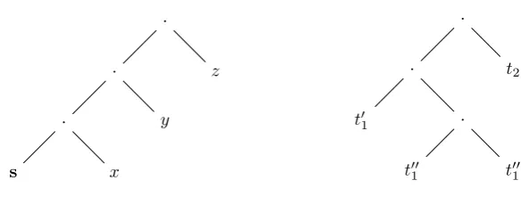
We will describe how we can check whether the combinator can be reduced with an example. Suppose we found the scombinator and we want to know whether the subterm is of the form s·x·y·z, or, whether there’s010101013hxihyihziwritten on the tape.
We need to make sure whether there are three separate subterms written after the 013. We start with x. That can be a combinator, or some application of two other termst1·t2.
s x
· y
· z
·
t001 t001 t01 ·
· t2
[image:30.595.155.447.100.215.2]·
Figure 6.1: Terms as trees
to the counter. Each time we read a combinator, we subtract one from the counter. If we read a combinator while the counter is at zero, then we’ve reached the end of the subterm. This works, since with every application, we allow for one extra combinator in the term. We then continue to check the next subterms this way, and we also denote the location of the beginning of them.
This process of checking a subterm needs time linear in the length of the string and thus also in the length of the term (using Lemma 6.1.2).
If what comes next is not correct for applying the axiom (so no hxihyihzifor some
x,y andz), we will go back to that combinator. This can also be done within linear time. From there we will go to the right again, looking for the next combinator, we denote the location of that one and we start again.
This process will repeat itself until we’ve found a combinator that we can rewrite (and if this doesn’t happen then we are done and we output what’s on the tape). We need to iterate this at most `(t) times. In order to find a combinator to rewrite we would thus use a number of steps that is polynomial in`(t).
We can now give the proof of the main theorem:
Proof of Theorem 6.1.1. Assume that we have a term t, and t →n z, with z in
normal form, where we always used the axiom for the leftmost combinator that could be rewritten.
By Lemma 6.1.4, we know that we can find the combinator for the reduction step of a term s in polynomial time. By Lemma 6.1.3, we know that every term that appears in the computation has length at most (n+ 1)`(t). So each time, finding the combinator that we will apply one of the basic axioms to will need time polynomial in (n+ 1)`(t).
Because we denoted the locations of the subterms that are going to get changed by the reduction, rewriting the term can also be done in polynomial time.
We then repeat this process ntimes. The entire computation can thus be done in
6.2 A term that simulates Turing machines
In this section we will describe how for each Turing machine, we can find a term that simulates that Turing machine.
We will adapt the Turing machine such that it is a machine with only one one-way infinite tape and that its computation halts when the head is located at the first bit of the output. For any Turing machine there exists another machine that is of this form and computes the same function with a polynomially bounded overhead in time [3, Ch. 1]. We also assume that the machine reads the entire input during the computation, which is often done in standard computational complexity.
We have that Γ is the alphabet with size l, that Qthe set of kstates, where q1 is the starting state andqk the halting state, and thatδ:Q×Γ→Q×Γ× {L, R, S}is
the transition function.
In order to describe a single configuration of the Turing machine during its compu-tation, we will use the following tuple of four [14]:
C= (q,[T(n)],[T(n−1), T(n−2), . . . , T(0)],[T(n+ 1), T(n+ 2), . . . T(n+m)]).
The symbolqwill be a number that represents the state of the Turing machine. T(n) is the symbol under the head of the Turing machine. The other lists describe the symbols before and after T(n).
In reality the Turing machine has an infinite tape, with an infinite number of “blank”-symbols going both sides, but we do not need to encode these in order to simulate the computation. We will denote the empty list by ’[]’, (see Section 5.5.1).
Assume that a Turing machine M will receive the input x∈ {0,1}n, and that it
runs in time f(n). We describe a term ∆ that will simulate the computation of the machine on input (0, x0,[],[x1, . . . , xn−1]).
Definition 6.2.1.
∆·C:= whenq1=C0
whenqk−1=C0
whenqk =C0
⇒
⇒
⇒
whenγ1=C1
whenγl=C1
pC1C3
⇒∆·(q, γ, C20, C30)
We cannot really perform recursion like this in ACT. However, using lambda ab-stractions and theF-combinator will unnecessarily complicate the description of this term. As we saw in Chapter 5, using this definition will have no influence on the complexity-analysis of the actual ∆’s.
Ci is shorthand forindCi(see Section 5.5.2), and for checking equality we will use
enm(Section 5.4.6).
1. Whenδ(qi, γj) = (qi0, γj0, L), then we put (qi0,p0C2,p1C2,pγj0C3).
2. Whenδ(qi, γj) = (qi0, γj0, R), then we put (qi0,p0C3,pγj0C2,p1C3).
3. Whenδ(qi, γj) = (qi0, γj0, S), then we put (qi0, γj0, C2, C3).
We will show that the term ∆ reduces to a term in normal form with a number of steps that is polynomial inf(n).
Theorem 6.2.1. For each TMM, there is a term tsuch that for x∈ {0,1}n,ACT`
t·x→mM(x), wherem is polynomial in the computation time ofM.
Proof. Let M be the Turing machine described in the beginning of this section. Assume thatM runs in timef(n).
It is clear that there exists a term that on input [x0, . . . , xn−1], in linear time
com-putes (q1, x0,[],[x1, . . . , xn−1]).
We will then give this to ∆, which will compute M(x). The rest of the proof will be a time-analysis of ∆.
Since there is a constant number of states, eachqiwill be a natural number bounded
by some constant. Since enm runs in time linear in min(n, m), we will have that checking the equality for the states can be done in constant time. The same holds for checking equality for the symbolsγi. Creating the new 4-tuple can also be done within
a constant number of steps for each input.
7 Complexity Results
In this chapter we will prove some results from standard computational complexity. As stated in Section 2.1.3, diagonalization is referred to as a relativizing proof-technique. However, we need more axioms before we can actually use diagonalization. Therefore, we will introduce an extension toACT. We then define several complexity classes, and deduce some results concerning those.
7.1 Universal computation
In order to use diagonalization, we need the following: 1. An enumeration of all programs
2. A program that can simulate other programs
We will formalize these two statements in several axioms. We introduce two ex-tra combinators: an encoding, enc, and its inverse, dec. We also have a universal combinator,u, that can simulate other terms.
U.1 ∀x∃n∈N[enc·x→1n∧dec·n→1x] U.2 ∀n∈N∃x[dec·n→1x∧enc·x→1n]
U.3 ∀n1, n2, n3, n4∈N∃m∈N[u·n1·n2·n3·n4→n2
1 m∧(m= 1∨m= 0)]
U.4 ∀nx, ni, nt, m∈N[(dec·nx)·ni→nt m⇒u·nt·nx·ni·m→1]
U.5 ∀nx, ni, nt, m∈N[¬((dec·nx)·ni →nt m)⇒u·nt·nx·ni·m→0]
The universal combinator is in some way able to tell us whetherx·ni→nt mor not,
even though this is not decidable in ACT itself. We also have that the first natural number that uis applied to, gives us a bound on the total computation time of u. The combinator eventually always outputs 0 or 1.
We call the system ACT together with these axioms and the symbols forenc,dec anduthe systemACT+U. Similarly, we haveACTf+U, where of course in the axioms U.1 until U.5 we use→f. We also have the following:
Corollary 7.1.1. For all total recursivef and for all formulasϕ:
7.2 Enumerating the terms
What seems useful in proofs that use diagonalization, is to actually have an enumera-tion of terms that satisfies the following properties:
i Every number represents a term.
ii Every term occurs infinitely many often in the enumeration.
The first property is satisfied by axiomU.2. We will use the following enumeration to satisfy the second property:
1. (1,1) 2. (2,1) 3. (2,2) 4. (3,1)
5. (3,2) 6. (3,3) 7. (4,1) 8. · · ·
We ensured that each number appears infinitely-many often on the right side of the pairs. We also have that for any numbers m and c, there exists a pair (k, m) in the enumeration such that c ≤ k. Later on, we will see that this is useful for diagonalization.
There is a program that on input n, gives the pair (k, m) from the enumeration in polynomial time. We will not prove this formally, but since we have that 1+2+· · ·+k=
k(k+1)
2 , the following algorithm will work:
enum(n ) : For i = 1 , . . .
i f n − i ( i +1)/2 <= i
i f n − i ( i +1)/2 = 0 o u t p u t ( i , i )
e l s e
o u t p u t ( i +1 , n − i ( i +1)/2)
Definition 7.2.1.
enum00:=λx.λn.λc.
d min(minn(div(timesi(succi))2))i d(e0(minn(div(timesi(succi))2))) (pii)
(p(succi)(minn(div(timesi(succi))2)))
xn(succi) enum0:=F·enum00
enum:=λn.enum0·n·1
We will assume that for any n, enum·n will give the pair (k, m) in polynomial time.
7.3 Complexity classes
In the system ACT, complexity classes are represented by formulas. We will only consider the complexity of terms that compute functions from N to N. A standard complexity class will look like this:
For a termt,Cg(t) holds when∃t0, t0
.
=tand∀n∈N∃m∈Ns.t. t0·n→g(n)m. The class of polynomial-time 0,1-valued functions can be described in the following way:
Definition 7.3.1. For a termt, P(t) is true when there exists a termt0, t=. t0, and constants c, c0, such that for all n ∈ N there exists an m, m = 0 or m = 1, and
t0·n→nc+c0 m.
There is a difference between the formulaP and the classPfrom standard compu-tational complexity. For the complexity, we consider functions that are polynomials in the input, instead of polynomials in the length of the input.
We defined the length of a natural numbernto ben+ 1, so we can consider this as functions in the length ofn. We could’ve chosen to consider functions as log(n)c+c0, to
capture the length of the binary string that representsn. However, choosing the actual natural number as input for the complexity bound gives complexities of for example addition and multiplication that are in correspondence with the Turing complexities of those functions.
We also have exponential-time computation:
Definition 7.3.2. For a term t, EXP(t) is true when there exists a term t0, t=. t0, and constants c, c0, such that for alln∈ Nthere exists anm, m = 0 or m= 1, and
We can describe a formula that is true when sis a binary sequence:
∃n, m[lens→n m∧ ∀i≤m(indsi= 0∨indsi= 1)].
With that, we will define nondeterministic polynomial-time as follows:
Definition 7.3.3. For a termt,N P(t) is true when for all nthere exists anm such that t·n→m0 ort·n→m1. We also need that there exists a termt0, constantsc, c0,
and a polynomial p, such that for all n ∈ N and binary sequencess of length p(n),
there exists an m,m= 0 orm= 1, such thatt0·(n, s)→nc+c0 m. We have that
∀n[t·n→1⇔ There exists a binary sequences(lens≤p(n)∧t0·(n, s)→nc+c0 1)].
We only focused on 0/1-functions in this section. The classesP andEXP could of course also be defined for all functions. This is however not possible forN P.
7.4 Time Hierarchy Theorem
We will outline how to reproduce the Time Hierarchy Theorem of Hartmanis and Stearns with ACT+U.
Theorem 7.4.1 ([8]). ACT+U`P 6=EXP
The original Time Hierarchy Theorem gives a sharper bound. The version that we prove here is easier to understand and gives the reader an impression of the proof-method that was used.
Proof.We will show the statement by actually showing the following ACT+U` ∃t[EXP(t)∧ ¬P(t)].
We lett=λn.d u·(plus·(exp·(p1(enum·n))·(p0(enum·n)))·(p1(enum·n)))·
(p1(enum·n))·(p1(enum·n))·1
0 1
. Or:
t (n ) :
enum ( n ) = ( k ,m)
I f u (mˆk + k , m, m, 1 ) −> 1 Output 0
e l s e
Output 1
So on input n, letenum·n→(k, m). The algorithm checks whether (dec·m)·m→mk+k1.
If yes, we output 0 and if no we output 1.
t=. t0 andt0·n→
nc+c0 0/1. By Axiom U.2 we have that there exists anmsuch that
dec·m→1t0. By the enumeration of the programs, we have that there exists annsuch thatenum·n= (k, m) andmc+c0≤mk+k. This means thatt0·m→1⇒t·m→0
andt0·m→0⇒t·m→1. Contradiction.
7.5
P
vs
N P
is independent from
ACT
+
U
In this section, we will show the following theorem: Theorem 7.5.1. P =N P is independent fromACT+U.
We will obtain this result by giving oraclesfA,fB such thatACTfA+U`P=N P
andACTfB+U6`P =N P. Then, together with Corollary 7.1.1, we have the theorem.
7.5.1 Relativized world where
P
=
N P
Lemma 7.5.2. [5] There exists a total recursive fA such thatACTfA+U`P=N P
The proof of this lemma is based upon [3, Th. 3.7].
Proof.We assume that we have a suitable encoding and decoding for triples, that can be computed within polynomial time, such that for anyn∈N, there existsx, y, z∈N
withn= (x, y, z).
We lettfA :=λ(x, y, z).u·(exp·2·x)·y·z·1. The decoding of the triple is part of
the computation of tfA·n. tfA will thus simulate a computation (dec(y) on inputz)
for exponential time (2x) and tell us whether the program accepted.
We can assume that ACTfA +U ` ∀x[P(x) ⇒ N P(x)].We will now argue that
ACTfA+U` ∀x[N P(x)⇒P(x)].
Assume that for sometwe have thatN P(t) holds. Then for alln,t·n→0/1. There also exists a termt0, constantsc,c0 and a polynomialp, such that for alln,t·n→1 iff there exists a binary sequence s such thatlens≤p(n)∧t0·(n, s)→nc+c0 1.
We can now make a make a termxas follows. On inputn, we enumerate all binary sequences of length at mostp(n). This can be done in exponential time. For each of such sequencess, we runt0 on input (n, s). This is done in polynomial time. If for one sequence t0 gives 1,xalso outputs 1. If this doesn’t happen for any sequence thenx
outputs 0.
In total,xruns in exponential time, say, 2q(n) for someq. We also have that there exists a term msuch thatenc·x→1m. With this, we can make a termy as follows. On inputn, encode a triple (m, q(n), n) and give this to the oracleofA. Then output
the same result. We have thatyneeds polynomial time for the computation, andy=. t.
7.5.2 Realizability with truth
We cannot actually use the known proof of Baker, Gill and Solovay in [5] to show that there exists a function fB such that ACTfB +U ` P 6= N P. This is because
our universal term does not allow us to have specific behaviour depending on what string is given to the oracle. Also, the creation of the oraclefBin several stages poses
a problem. However, with results from Chapter 6, on the invariance of ACT with respect to Turing machines, we can argue for the existence of a term that acts as a universal machine and has somewhat more flexibility with respect to its behaviour. We will show the following theorem, which still depends on results from [5]:
Theorem 7.5.3. There exists an oraclefB and a termtsuch thatACTfB+U`N P(t)
but ACTfB+U6`P(t).
This theorem is implies thatACTfB+U6`P =N P. However, some of the reasoning
in the proof can thus only be done in the meta-theory. In order to obtain a contra-diction after assuming thatACTfB+U`P(t), we need to make sure that statements
from ACTfB+U about terms also extend to the meta-theory. We thus first need to
show the following:
Lemma 7.5.4. WhenACTf+U` ∃xϕ(x), then there exists a closed termt such that
ACTf+U`ϕ(t).
We will do this by using realizers. First, for any formula ϕ, we define another formulax rt ϕas follows:
Definition 7.5.1.
x rt φ:=φifφis an atomic formula
x rt (φ∧ψ) :=p0x rt φ∧p1x rt ψ
x rt (φ∨ψ) := (p0x= 0⇒(p0p1x)0 rt φ)∧(p0x6= 0⇒(p1p1x)0 rt ψ)
x rt (φ⇒ψ) := (φ⇒ψ)∧ ∀y(y rt φ⇒x·y rt ψ)
x rt ∃yφ:=p1x rt φ(p0x)
x rt ∀yφ:=∀y(x·y rt φ)
We can now turn to the proof of the lemma. Since the proof is quite similar to how this is shown other systems, such as for HA∗ in [6], we will not fill in all the details. Proof sketch. We will first show thatx→ny andy rt ϕimplies thatx rt ϕ.
This is done with induction on the complexity of ϕ. When it is an atomic formula then the statement obviously holds. Wheny rt ϕ andϕ:=φ∧ψ, then by definition p0y rt φandp1y rt ψ. We have that x→n y implies thatp0x→np0y. So by the induction hypothesis, also p0x rt φ. The case forp1y is similar.
We have that for any ϕwithout free variables, if ACTf+U`ϕthen there exists a closed termtin the language ofACTf+Usuch thatACTf+U`t rt ϕ. This can be shown by giving terms that realize the axioms. For implications we show that realizers for the premises give us realizers for the conclusions.
The combinators are realized by themselves. The axiom for induction can be realized with the following termi:
i0:=λxλyλzd(z)(p1y·(pred·z)·(x·y·(pred·z)))(p0y)
i:=F·t
Now assume thatACTf+U` ∃xϕ(x). Then there exists anssuch thatACTf+U`
s rt ∃xϕ(x). So, by definition, p1s rt ϕ(p0s). If we let t = p0s, then the lemma
follows.
7.5.3 Relativized world where
P
6
=
N P
We will first describe how we can construct a universal term. Take the Turing machine that simulates computations of terms, Theorem 6.1.1. Then simulate this Turing machine with the term that simulates Turing machines, Theorem 6.2.1. We now have such a universal term u0.
What’s more, this term simulates other terms with only a polynomial overhead in time. Recall the encoding of terms as binary strings, Definition 6.1.1. Note that we can decide whether a binary string encodes a valid term. We can decide to let u0
immediately output 0 on strings that do not encode a term. Then we also have that the representation of terms as binary strings satisfies the following two criteria:
i Every binary string represents a term.
ii Every term is represented by infinitely many binary strings.
We can also make a termu00 that works asu0 only it can also readof-combinators
for a specific f, with an obvious modification to the binary representation of terms. We can expand the universal term even more, by giving it a counter to keep track of the reduction steps that are done. This way we can give an additional natural number as input and let the universal term simulate for at most that many steps.
There is one problem: for the proof we need that the oraclefBis actually a function
that takes binary strings as input. As was argued in Section 7.3, there is a formula that can tell us when a term is a binary string. We need to alter the axiom for the of-combinator such that it also allows for oracles that are functions in binary strings.
Thus, letf(x) denote the output off on inputx. Then:
We can now mimic the known proof of Baker, Gill and Solovay to show Theorem 7.5.3:
Proof sketch. We will define a termtfBthat computes functionfB, and for all binary
sequences x, decide whether fB(x) = 1 (tfB·x→1) or fB(x) = 0 (B·x→ 0). We
will do this in several stages. During this process, we need to keep track of sequences which we already considered. We will do this by updating list,L, that contains binary strings. We ‘remember’L using recursion.
The rest of the proof then proceeds as outlined in for example [3, p. 74].
The idea is as follows. We will look at the functiongthat on inputn, gives 1 when there is a binary sequence xof length nwith and tfB·x→ 1. If there isn’t such a
sequencextheng(n) = 0.
There exists a termtthat computes this functiongwithACTfB `N P(t). This is
because we can create a termt0 that gets as an input annands, computesofB·sand
outputs the result.
We will now definetfB such that we cannot have thatP(t) holds. We do this with
diagonalization, for several stages.
In stagei, with the universal term, we can simulate a term ti represented by string
i on some inputni for 2
ni
10 steps. We chooseni such that it is bigger than the strings that we’ve previously put in the list L. During the computation, ti can query the
oracle for several strings, but at most 210ni many of them, so there are always strings of length ni that ti cannot query. If i halted within that time, then depending on
whether ti·ni →1 or ti·ni→0 we can decide to put a string that it hasn’t queried
in the listLor put no strings of lengthniin L. We make sure thatti gives the wrong
answer on whether there exists a string of lengthni inL or not.
The term tfB then runs as follows: on input x∈ {0,1}
n it goes through all stages
starting from 1 until we simulate a term on an inputni ≥n. It then checks whether
x∈L or not and outputs 1 or 0 accordingly to the answer. SotfB·x→1⇔x∈L.
By our construction ofLandtfB, we have that all terms that run in polynomial-time
have at least one input on which it differs withg.
So, when we assume thatACTfB+U`P(t), we have inACTfB+Uthat there exists
a t0, t0 =. t, and that there exists constants c, c0, such that for alln ∈Nthere exists an m,m= 0 or m= 1, andt0·n→2nc+c0 m. Then, by Lemma , we have that there
exists a closed term t00 such that inACTfB +U the above holds. However, this is in
contradiction with our construction of tfB.
We can conclude that there exists a term t such that ACTfB +U ` N P(t) and
ACTfB+U6`P(t).
7.5.4 Independence result
Lemma 7.5.5. ACTfB+U6`P=N P
Assume, towards a contradiction, that ACTB+U ` P =N P. Then we also have that ACTB+U ` ∃x[t =. x∧P(x)]. With Lemma 7.5.3, we have that there exists a termssuch thatACTB+U`t=. s∧P(s). Contradiction.
Theorem 7.5.6. P vsN P is independent ofACT+U
Proof.Suppose thatACT+U`P =N P orACT+U`P 6=N P. Then, by Corollary 7.1.1, for all f, also ACTf +U ` P = N P or ACTf +U ` P 6= N P. But this is in
contradiction with lemmas 7.5.2 and 7.5.5.
8 Conclusion
We’ve presented a system, ACT, in which we can express the complexity of solving problems. Everything that can be proven inACT also relativizes.
The system uses combinatory logic to perform computations and it is invariant with respect to Turing machines.
A small extension of the system enables us to reason about computations relative to oracles. For any total computable functionf, there exists the systemACTf, where all computations are relative to the oracle f. Any proof inACTcan also be done within ACTf for any f, which ensures that all proofs fromACTrelativize. Both the systems ACT andACTf are consistent.
InACT, we are only able to consider the time-bounded complexity of functions. It would be interesting to extend the system such that it can also express space-bounded complexity. The length of a term seems to be a good measure for this, and also allows for an orthodox interpretation of the invariance thesis (a single simulation achieves the polynomial overhead in time and constant factor overhead in space bounds). However, ACT is not able to talk about the length of its own terms.
A way of defining nondeterministic and probabilistic computations is also something to consider in future work. With probabilistic computations we can try to say more about proof-methods such as arithmetization, which is regarded as non-relativizing.
An important thing to note is thatACT cannot tell us which proof-methods donot
relativize. We can only be sure that statements that can be proven within ACT are relativizing. Still, it is expected that we can obtain information on non-relativizing techniques with further studies.
But even then, it is difficult to mimic all proofs of standard computational complex-ity, since a lot of proofs are dependent on the exact workings of a Turing machine. To mimic the proof of the construction of the oracle relative to which P 6=N P we had to use binary sequences. The proof could also not be done within the system itself, but only in the meta-theory. It would be better when this was possible within ACT and when we could construct an oracle that worked for natural numbers, instead of an oracle for binary sequences.
In this work, we only used computable oracles. This was more in line with the constructive approach that we wanted to take. Besides this, in standard computational complexity almost all oracles that are used are actually computable.
We also chose to only have total functions as an oracle, even though perhaps par-tial functions would’ve worked as well. We did this, because it fits nicer with the requirement that the oracle is computable.
9 Acknowledgements
In the process of writing this thesis, my two supervisors where the most important. I would like to thank Benno van den Berg for giving me the idea to create this formal system. I also want to thank him for answering the numerous questions that came up throughout the whole process, even though he had perhaps too many other things to do. I also have lot of gratitude towards Leen Torenvliet. No matter the topic, he was always able to give me related papers to expand my background knowledge. But most of all, he was very supportive and believed in me, even when I didn’t do this myself. I hope that in the future there will be more opportunities to collaborate with the both of them.