Abstract: with day by day increasing population and standard of human being increases the consumption of electrical energy and this increasing in the consumption of electrical energy, increases the number of generators, transmission lines to full fill the daily needs of the electrical energy. So the power system has become more complex and main source of gaseous emission. So arranging and the task of intensity framework of power system must be done in such a way that energy and emission arising due to power generation, the retribution paid by the power plant because of emission and cost paid in generation need to tackle all the while. This paper shows a reliable and effective hybrid of particle swarm optimization (PSO) algorithm and teaching learning based optimization (TLBO) for combined emission and economic dispatch (CEED) problems. The outcomes have been shown for combined emission and economic dispatch issues of standard 3 and 6-generators frameworks with consideration of transmission losses.
Index Terms: Economic dispatch, Emission dispatch, PSO, TLBO, PSO-TLBO
I. INTRODUCTION
With the consideration of CEED dispatch problems of a thermal power plant, the basic or primary objective is to schedule the generating units’ outputs is such manners that satisfy all the system constraints that may be equality or inequality constraints and meet the load demand at minimum
generating power, minimum emission, minimum
environmental cost and operating cost. In recent years, emission and environmental limitation started to be considered as part of electric system planning and operation. So consideration of emission and environmental constraint with economic is very important in the case of power generation from thermal power plant. However, it became necessary for power utilities to count this. So this emission and environmental must be considered together with the economic. If we considered emission and environmental together CEED dispatch problems acts as multi-objective problem with highly linear and nonlinear constraints.For economic, reduction in emission, reduction in environment cost and power management lot of researches have been carried out till the date. Different derivative approaches applied to solve for the significant benefits in economic, reduction in emission, reduction in environment cost and power management including Lagrangian multiplier method [1].
Revised Manuscript Received on July 09, 2019
Rajanish Kumar Kaushal, Pursuing Ph.D. in Electrical Engineering Department of the Punjab Engineering College, Chandigarh, India Praveen Saini, Pursuing Ph.D. in Electrical Engineering Department of the Punjab Engineering College, Chandigarh, India
Dr. Tilak Thakur, Professor, Electrical Engineering Department of the Punjab Engineering College, Chandigarh, India
These methods only considered the incremental fuel cost curves that’s nature are monotonically increasing but actual curve is different from the monotonically increasing nature [2,3]. An ELD issue can be resolved with valve-point discontinuities by dynamic programming [4]. The issue of dimensionality, however, is the DP technique which imposes huge calculation burdens. Many population-based optimization methods like CASO (Caotic Ant Swarm Optimization) [5], evolutionary programming [6], hybrid evolutionary programming (HEP) [7], genetic algorithms [8–10], Simulated annealing [11], PSO [12-15], and have been used to solve complicated ELD-related issues in latest years.
II. PARTICLE SWARM OPTIMIZATION (PSO) Behavior of swarms motivated the main concept of the PSO. To better understand the PSO we can assume that a swarm of birds of fishes searching for the food randomly in a specific region. We can assume that all the birds or fishes are searching the same food in the search space. During the searching of food, each bird or fish has a position and velocity. Swarm of birds or fish schooling moves in such a way that they have the knowledge of distance of food but not the knowledge of the exact location of food. Best plan to get the food by birds or fishes to follow a bird or fish nearest to the food. In PSO each bird or fish acts as a particle and may be the solution within the ask for area, so the number of particle in the problem is equal to total numbers of birds and fishes and the total number of the particle shows the population size. Each particle within ask for area has its hold own velocity and fitness value. The fitness of any particle is determined by the objective function of the problem.
Steps to be taken to implement PSO algorithm:
1. Start with a swarm /population decision that depends on problem complexity.
2. For the position and velocity of the particles, initialized
randomly the particles.
3. The position of an ith particle is an array of 1X N in an N dimensional optimization problem.
P
i= [Pi1, Pi2,……….P
iN] (1)
Similarly velocity is presented by,
V
i= [Vi1, Vi2,……….V
iN] (2)
Combined Emission and Economic Dispatch
Problems using Hybrid of Particle Swarm and
Teaching Learning Based Optimizations
Figure1 Flow chart of PSO algorithm
4. The objective function given is to assess fitness for e ach particle:
F
i= f (Pi1,……….Pi2,…….P
iN) (3)
5. Two best positions are chosen for the next iteration, known as pbest and gbest.
Pbest: best personal position ever obtained by a Particle.gbest: best position in all pbests globally. In the case of a first iteration, pbest is the same as a random initial part, whereas in the case of subsequent iterations, pbest is the most appropriate for that particular iteration
6. Each particle’s velocity is updated with the following equation
1
1 2
1 2
k k k k
k k k
i i
pbest
ip
igbest
ip
iv
v
c
r
c
r
(4)Where:
k i
v
: ith particle velocity at k iteration.k i
: Weight of inertia at iteration k. c1 and c2: acceleration coefficients. r1 and r2: random numbers between (0, 1).k
i
pbest
: ith particle best position at iteration k. ki
p
: ith particle position at iteration k. ki
gbest
: Global best position at iteration k k1i
v
: Updated velocity at iteration k+1At the kth iteration the velocity
v
ki of ith particle should be within its minimum and maximum range:v
iminv
ki v
imax(5)
At each iteration, the inertia weight is modified by the next equation:
max min
max
max
k k
iter
(6)Where:
max
: Maximum inertia weight valuemin
: Minimum inertia weight valuemax
iter
: Maximum iteration number7. The After an updated velocity, the position of every particle is updated with the next equation.
k k 1 ki
i i
p
p
v
(7) 8. Fitness is assessed for each particle's updated locatin;pbest and gbest for the next iteration are achieved The process shall be repeated until a criterion of convergence is met.
Figure1 shows the step-by step process to implement the particle swarm optimization algorithm.
III. TEACHING LEARNING BASED OPTIMIZATION (TLBO)
TLBO is a one of the most effective and reliable intelligence algorithm for non convex optimization problems proposed by Rao etc in 2010 [5]. TLBO works in two important phases for optimizing a problem. The first important phase is instructor phase and second important phase is student or learner Phase. Initialize random position and
velocity of all particles. Start
For each particle position “P”, Evaluate fitness f (P)
First iteration?
For each particle, if f(P) is better than(Pbest) then Pbest=“P”
Convergence satisfied
End
For each particle, set pbest is equal to
its position “P”
Pbest Set as Gbest
Figure2 Flow chart of TLBO algorithm
By simulating the teaching and learning method it achieves improvement. This technique is incredibly easy as a result of having just one parameter that's the amount of learners and having the good performance and less optimization time because of single depending parameter. Because of its unique nature it is widely used in different practical problems and engineering problems. Researchers adopt varied improvement techniques to accurately simulate the teaching and learning method to urge improves performance. At each iteration the best technique is the greatest learners are selected since the best solutions in order to replace the least students also to increase the ability associated with global search also to keep up with the diversity of search the feedback process is launched after learning process.
TLBO has two fundamental amounts. The first is "Instructor Phase" as well as the second the single is "learner Phase".
The point by point process is depicted as pursues:
Stage 1: Define the enhancement issue and introduce the advancement parameters.
Stage 2: Initialize the populace Stage 3: Instructor stage Stage 4: Learner stage
Stage5: Terminate the calculation if the most extreme age number is accomplished, generally rehash from Step 3. The population of TBO alternatives is regarded to be one class of learners and the fitness of the alternatives is deemed to be results and grades. Through teacher learning and learning through the interaction between learners algorithm adeptly each class learner's grade updates. For the teacher group in its entirety, a teacher is the best solution. Teacher exchanges his / her experience with learners in order to improve median school performance. If xi =
(xi1…………..xid………xiD) is the position of the learner, the learner with the best fitness is identified as the teacher, and the mean position of a class with the NP learner is presented as:
1
1 (
NP
mean i
i
NP
x
x
(8)
Every learner's position is updated with the following equation:
x
i,new= x
i,
old+rand.(x
teacher-T
F.x
mean)
if the learner new and old positions are
x
i,new=(x
i,new1
…….
x
i,newd
…….. x
i,newD
)
and
x
i,
old= (
x
i,
old1
……..
x
i,
old d...
x
i,
oldD
)
, respectively, then a random vector distributed uniformly inside [ 0, 1 ] is the teacher's factor T (F).otherwise xi,new, is recognized unaffected when xi,new better thanx
i,
old .In the student stage, a student interacts randomly with other students in order to improve his/her efficiency. Learner xi selects another student xj randomly and the following equation can be used to express:
.(
),... ( )
(
)
,
.(
),... ( )
(
)
old
i i j i j
old
i j i i j
rand
f
f
i new
rand
f
f
x
x x
x
x
x
x
x
x
x
x
(9)
if f(x) is the objective function ,the ancient situation of the jth student is with D-dimensional variables is used in the replacement of xi, old,if xi, newis better than xi, old
IV. HYBRID PSO-TLBO OPTIMIZATION TECHNIQUE
For making the hybrid of the PSO and TLBO the concepts of the PSO and TLBO are used. At the first step generate the population as per problem and based on the population calculate the fitness for each and set the best of pbest as gbest on next apply teacher phase of TLBO in teacher phase choose the best solution for teaching and modified working solutions through teacher learning then apply PSO and update pbest as gbest and then apply student phase or learner phase of TLBO. When results are compared with the PSO and TLBO the Student
Phase
Modify possible solutions through mutual interaction in
the learning of students
Select two feasible solutions randomly
Generate new populations
Termination criterion
Satisfied
Select optimum
solution
Initialize Parameters
Population of Feasible solutions Solutions
Fitness Evaluation
Arrange Feasible Solutions according to
their Fitness Values
Teacher Phase
Modifies workable solutions t hrough teacher learning
hybrid of PSO-TLBO gives the improved results because it optimizes three times one in teaching phase second by PSO and third in student phase.
Figure3 Flow chart of hybrid (PSO-TLBO) algorithm
V. MATHEMATICAL PROBLEM FORMULATION
The formulation of CEED dispatch of a Thermal Power system summarized as:
Problem includes –
Economic optimization
Emission
optimization
Environmental Cost optimizationFor CEED dispatch problems, the following objectives and limitations are considered:
A) Economic optimization
i) Economic load dispatch for convex system
1 i
NT 2
= a + +C
FT Pgi iPgi b Pi gi i
$ / h
(10)
(ii) For non-convex system
1
2
min $ /
*sin
*
-T C
N
i i gi i gi i i i i i
h
F
a
P
b
P
c e
f
P
P
(11) Where:
FC (Pgi): is the total cost of fuel required for generation in ($/hr), ai, bi, and ci are cost coefficients of the ith generating unit and Pi represents the to the power generated by the ith unit.NT is the total number of units.
B) Emission Dispatch
( )
E
F Pgi : Represents the total emission of the thermal units in kg/h.
2
1
/
T
i
N
E gi
d
i gie
i gif
ikg hF
P
P
P
(12)di,ei,,fi,: are the emission coefficients of the ith generator
NT : Represents the total available committed thermal
generating units.
C) Environmental Dispatch
FHE (Pgi): spoken to as the all out expense as a result of health and environmental harm.
&
1
( ) ( )
T
H E gi gi
i
N
F
P
P
(13) D) Real power balance constraint
1 T
gi D L
i
N
P
P
P
(14) PL: represents the total transmission losses in the network and the total transmission losses can be represented by using B-coefficients as given below:00
1 1 1
T T T
L gi ij gj io gi
i j i
N N N
P
P B P
B P
B
(15)Here Bij, Bi0 and B00 are loss coefficients. E) Generation unit capacity limits
P
mingi
P
gi
P
maxgi (16) Pgimin
Represents the Minimum loading limit and on the other hand Pgimax represents the upper limit.
F) Ramp Rate Limits
Ramp rate limit such a limit, to the point that decide the range inside this generation may increment or decline. The thermal
unit generation limited by the ramp rate is limited by:
-1
-
-1-t t UPR Pi Pi i
t t
Pi Pi DPRi
(17)
Where UPRi represents upper limit of the ith unit and DPRi represents the down limits of the ith unit individually. Due to the limits of ramp rate generating units are expressed as:
-1
max(Pimin,UPRi-Pti)Pitmin(Pimax,Pit -DPRi) (18) F) Prohibited zones Limits
During the power generation each unit must be avoid operation in prohibited zones. The operating zones of the ith unit may be described as follows:
min
,1
l
gi gi gi
P
P
P
Select optimum
solution Criterion
Satisfied Generate
new populatio
n
Update pbest and gbest Start
Generate Population with considering the problem
Set best of pbest as gbest
Apply teacher phase of TLBO
Calculate population mean
Compare the result for best teacher
Apply PSO
, 1 , , 2, 3,... i
u l
gi j gi gi j j
n
P
P
P
(19)max ,
i
u
gin gi gi
P
P
P
Where:
nj: number of prohibited zones of ith generating unit;
, l
gi j
P
: lower active power limit of prohibited zone of j of ith generating unit, MW;, 1 u
gi j
P
: upper active power limit of prohibited zone of j-1 of ith generating unit, MW.VI. OPTIMIZATION PROBLEMS CEED dispatch issue of a Thermal Power Plant can be characterized as,
Minimize (
&
[( ( ) ( )), ( )]
C gi H E gi E gi
F P
F
P
F P
(20)Considering the constraints given in (14) to (19)
Mathematically, the fitness function of CEED can be described by introducing a price penalty factor as follows:
&
( C( gi) H E( gi)) * E( gi)
TC
F P
F
P
hF P
(21)VII. SIMULATION AND RESULT
The algorithm proposed is used in four various samples and contrasts with the demographic optimization methods used by past scholars such as NR, Tabu search, GA, NSGA, FCGA, DE and PSO. The performance of each system has been judged out of 50 trials. The programming was written in MATLAB language, using MATLAB 7.1 on Intel's earlier Core Duo processor, 1.6 GHz with 3GB RAM.
Case-I: To take a look at the adequacy of the PSO-TLBO algorithm first, three- units of a generating plant to meet total load of 850 MW is considered for this example. The framework information is the indistinguishable as [16].Here solely targets mainly emission & fuel fee is used for this situation. The performance of PSO-TLBO is compared to that of Tabu search [24] and non dominated sorting genetic algorithm-II (NSGA-II) [17].
Table 1 Generating unit capacity and coefficients for case-I
Unit Pimin Pimax ai ($)
bi ($/MW)
ci ($/MW2)
1 150 600 0.001562 7.92 561
2 100 400 0.00194 7.85 310
3 50 200 0.00482 7.97 78
Table2 Emission coefficients for case-I Units f (lb/h) e (lb/MW/h) d (lb/MW2/h)
1 13.85932 0.32767 0.00419
2 13.85932 0.32767 0.00419
3 40.26690 -0.54551 0.00683
Table3 Best compromise solution for case-I
Unit Tabu
search [16]
NSGA -II [17]
BBO [21]
PSO- TLBO
P1(MW) 435.69 435.88 435.195 436.07
P2(MW) 298.82 299.98 299.972 223.46
P3(MW) 131.28 129.95 130.662 200
TG(MW) 865.79 865.82 865.829 859.56
TL(MW) 15.798 15.826 15.8290 9.56 FC($/h) 8,344.5 8,344.5 8,344.59 8337.6
E(kg/h) 0.0986 0.0986 0.09869 0.0442
0 100 200 300 400 500
1.486 1.487 1.488 1.489 1.49 1.491 1.492
1.493x 10
4
Iterations
T
ot
al
c
os
t i
n
($
/h
)
Figure4 Total Cost Variation for 3-Units System Case-II: In the second case to demonstrate the deliberate algorithmic six power generating units having price and emission in the form of quadratic equation is taken into account. All the information is taken from [17].
Table 4 Generating unit capacity and coefficients for case-II
Unit Pimin Pimax ai ($)
bi ($/MW)
ci ($/MW2)
1 10 125 756.88 38.53973 0.15247
2 10 150 451.32 46.15916 0.10587
3 35 225 1049.9 40.39655 0.02803
4 35 210 1243.5 38.30553 0.03546
5 130 325 1658.5 36.32782 0.02111
6 125 315 1356.6 38.27041 0.01799
Table5 Emission coefficients for case-II Units f(lb/h) e (lb/MW/h) d(lb/MW2/h)
1 13.85932 0.32767 0.00419
2 13.85932 0.32767 0.00419
3 40.26690 -0.54551 0.00683
4 40.26690 -0.54551 0.00683
5 42.89553 -0.51116 0.00461
6 42.89553 -0.51116 0.00461
Table6 loss coefficients for case-II
0.002022 0.000286 0.000534 0.000565 0.000454 0.000103
0.000286 0.003243 0.000016 0.000307 0.000422 0.000147
0.000533 0.000016 0.002085 0.000831 0.000023 0.000270
0.000565 0.000307 0.000831 0.001129 0.000113
B
0.000295
0.000454 0.000422 0.000023 0.000113 0.000460 0.000153
0.000103 0.000147 0.000270 0.000295 0.000153 0.000898
[image:6.595.47.559.219.379.2]
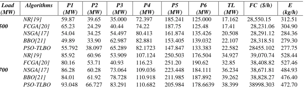
Table 7 Best compromise solution for case-II Load
(MW)
Algorithms P1
(MW)
P2 (MW)
P3 (MW)
P4 (MW)
P5 (MW)
P6 (MW)
TL (MW)
FC ($/h) E
(kg/h)
500
NR[19] 59.87 39.65 35.000 72.397 185.241 125.000 17.162 28,550.15 312.51
FCGA[20] 65.23 24.29 40.44 74.22 187.75 125.48 17.41 28,231.06 304.90
NSGA[17] 54.04 34.25 54.497 80.413 161.874 135.426 20.508 28,291.12 284.36
BBO[21] 49.89 33.90 62.987 82.881 153.405 139.032 22.107 28,318.51 279.30
PSO-TLBO 55.792 38.097 65.289 82.1723 147.847 133.383 22.582 28455.102 277.75
700
NR[19] 85.92 60.96 53.909 107.124 250.503 176.504 34.927 39,070.74 528.44
FCGA[20] 80.16 53.71 40.93 116.23 251.20 190.62 32.85 38,408.82 527.46
NSGA[17] 86.28 60.28 73.064 109.036 223.448 184.111 36.234 38,671.81 484.93
BBO[21] 84.01 61.92 78.728 110.918 211.985 187.892 39.262 38,828.27 476.40
PSO-TLBO 93.048 66.727 83.291 110.682 205.984 178.6639 38.399 38998.303 472.70
Case-III In this case, six generating units with ramp rate limit and prohibited zones constraints of all units are considered to check the adequacy of the PSO-TLBO algorithm for combined economic emission dispatch. The data are used from [21] for cost coefficients, active power limits, ramp rate limits, and prohibited zones. Table 8, 9 provides information of cost and emission coefficients. Table 10 provides the prohibited zones and ramp rate limit and table 11 provides loss coefficients.
Table 8 Generating Unit Capacity And Coefficients For Case-III
Unit Pimin Pimax ai ($)
bi ($/MW)
ci ($/MW2)
1 100 500 240 7.0 0.0070
2 50 200 200 10.0 0.0095
3 80 300 220 8.5 0.0090
4 50 150 200 11.0 0.0090
5 50 200 220 10.5 0.0080
6 50 120 190 12.0 0.0075
Table 9 Emission Coefficients For Case-III Units f (lb/h) e (lb/MW/h) d (lb/MW2/h)
1 13.85932 0.32767 0.00419
2 13.85932 0.32767 0.00419
3 40.26690 -0.54551 0.00683
4 40.26690 -0.54551 0.00683
5 42.89553 -0.51116 0.00461
6 42.89553 -0.51116 0.00461
Table10 Prohibited zones and ramp rate limits for case-III
Unit Prohibited zones MW)
Pi0 UPRi DPRi
1 [210 240][350 380] 440 80 120
2 [90 110][140 160] 170 50 90
3 [150 170][210 240] 200 65 100
4 [80 90][110 120] 150 50 90
5 [90 110][140 150] 190 50 90
6 [75 85][100 105] 110 50 90
Table12 Simulation Result of 6-Grnerator System With Different Algorithms For Case -III
0 100 200 300 400 500
2.1 2.2 2.3 2.4 2.5 2.6 2.7x 10
4
Iterations
T
o
ta
l
c
o
st
($
/h
) Operating Cost for 1000 MW Load
Figure5 Total Cost for 1000 MW load case-III
Case-IV: In this case, six generation units with ramp-rate limit and prohibited zones constraints of all units
are considered to check the adequacy of the PSO- TLBO algorithm for combined economic emission dispatch with additionally constraint environmental cost constraints. The all data is same as the case –III additionally data required for the for the case-iv that is coefficient of health and environmental damage CHE
That depend on the power generated by thermal power plants here CHE is assumed as 100 $/MWh. It is observed that major part of the optimized cost corresponding to each level of power demand is the cost paid for health and environmental damage that damage caused because of emission from the thermal units. So it needs to pay this part by thermal power plant to compensate the health and environmental damage because of emission. Case-iv is considered for three loads
that’s are 1000 MW, 1200 MW and 1500 MW. Here TEC represents the total environment cost in $/h.
Table13 Best Compromise Solution For Case-IV Unit PSO-TLBO
1000(MW) 1200(MW) 1500(MW)
P1(MW) 320.0071 344.4352 394.2155
P2(MW) 161.9398 200 200
P3(MW) 130.0942 209.9895 244.8919
P4(MW) 79.70434 133.1488 150
P5(MW) 193.7819 200 200
P6(MW) 119.9045 120 120
TG(MW) 1005.4319 1207.5735 1309.1074
TL(MW) 5.3104 7.5718 9.1074
PF 53.5198 110.3852 110.3852
TC($/h) 198446.97 437312.52 537253.19
FC($/h) 12169.261 14665.460 15939.178
E(lb/h) 1601.9218 2734.8754 3536.7364
TEC($/h) 100543.19 120757.34 130910.73
VIII. CONCLUSION
The paper provides Hybrid optimization based on the particles of swarm and teaching learning to solve the four-case problem of the combined economic emission of load dispatch. In the first case, PSTLBO offers the best fuel price among all its algorithms, and also finds that its best emission alternatives are similar to those found in Tabu search and NSGA. In all three cases of load demand, a system of 6 Generators, not including prohibited zones and raffle-ramp limitations (second example) shows similar fuel costs with a range of algorithms and significantly improves emissions level with PSTLBO. Non-linear property such as ramp rate limits and forbidden zones are provided for the practical operation of thermal generators and it is noted that the proposed algorithm has a better performance than other best-known methods such as the GA and PSO.
In the recent CEED problem, PSTLBO shows a smaller full (goal) importance relative to PSO
and GA in the third case. Given all Units
Algorithms
DEMAND (1000 MW) DEMAND (1200 MW)
GA PSO BBO[21] PSO-TLBO GA PSO BBO[21] PSO-TLBO
P1(MW) 320.0 320.00 320.00 320.1186 329.1083 329.6465 349.216 330.4007
P2(MW) 140.00 164.61 160.00 162.6623 198.0966 198.1324 200.000 197.3993
P3(MW) 142.14 138.10 137.77 137.3499 243.8283 240.0493 211.779 240.0173
P4(MW) 90.000 77.37 80.000 79.55501 121.3974 124.792 131.000 120.3688
P5(MW) 197.50 189.98 191.82 185.4665 199.8071 199.5031 200.000 199.6839
P6(MW) 119.99 119.50 120.00 119.9956 119.4460 119.9729 120.000 119.9663
TG(MW) 1,009.6 1,009.58 1,009.6 1005.1479 1,212.172 1,212.116 1,211.99 1207.8365
TL(MW) 9.6489 9.5813 9.6084 5.0663 12.1823 12.116 11.9964 7.7992
PF 6.1152 6.1152 6.1152 6.1152 12.8718 12.8718 12.8718 12.8718
these results, the proposed algorithm is ultimately perfect for near-ground optimization in terms of combined economic and emission dispatch issues with different loads, restrictions and costing functions.
REFERENCES 1. Wood AI,Woolenburg BF (1996) Power generation operation and
control. Wiley, New York.
2. D.J. Kothari and J.S. Dhillon, Power System Optimization, New Delhi, India: Prentice-Hall of India Pvt.Ltd, 2004, pp. 572.
3. Nanda J, Hari L, Kothari ML (1994) Economic emission load dispatch with line flow constraints using a classical technique. IEEProc Gen Transm Distrib 141(1):1–10.
4. Shoults RR et al (1986) A dynamic programming based method for developing dispatch for developing dispatch curveswhen incremental heat rate curves are non-monotonically increasing. IEEE Trans Power Syst 1(1):10–16.
5. Cai J, Ma X, Li L, Yang Y, Peng H, Wang X (2007) Chaotic antswarm optimization to economic dispatch. Electr Power Syst Res77:1373–1380
6. Park JH, Yang SO, Lee HS, Park YM (1996) Economic load dispatch using evolutionary algorithms. In: Proceedings of the international conference on intelligent systems applications to power systems, pp 441–445 (1996)
7. Swain AK, Morris AS (2000) A novel hybrid evolutionary programming method for function optimization. In: Proceedings of the 2000 congress on evolutionary computation, vol 1, pp 699–705
8. Chiang C-L (2005) Improved genetic algorithm for power economic dispatch of units with valve-point effects and multiple fuels. IEEE Trans Power Syst 20(4):1690–1699
9. Walters DC, Sheble GB (1993) Genetic algorithm solution of economic dispatch with valve point loading. IEEE Trans Power Syst 8:1325–1332 10. He H, Sykora O, Salagean A, Makinen E (2007) Parallelisation of genetic algorithms for the 2-page crossing number problem J Parallel Distrib Comput 67(2):229–241
11. Abido MA (2000) Robust design of multi-machine power system stabilizers using simulated annealing. IEEE Trans Energy Convers 15(3):297–304
12. Kennedy J, Eberhart R (1995) Particle swarm optimization. IEEE Int Conf Neural Netw, pp 1942–1948
13. Boeringer DW, Werner DH (2004) Particle swarm optimization versus genetic algorithms for phased array synthesis. IEEE Trans Antennas Propag. 52:771–779
14. Lu H, Sriyanyong P, Song YH, Dillon T (2010) Experimental study of a new hybrid PSO with mutation for economic dispatch with non-smooth cost function. Int J Electr Power Energy Syst 32(9):921–935
15. Abido MA (2009) Multiobjective particle swarm optimization for environmental/economic dispatch problem. Electr Power Syst Res 79(7):1105–1113
16. Roa-sepulveda CA, Salazar-Nova ER, Graciacaroca E, KnightUG and Coonick A (1996) Environmental economic dispatch viaHopfield neural network and taboo search. UPEC’96 Universities Power Engineering Conference, Crete, Greece, pp 1001–1004(1996).
17. Rughooputh Harry CS, King Robert TFAh (2003) Environmental/economic dispatch of thermal units using an elitist multi-objectiveevolutionary algorithm. ICIT Maribor, Slovenia, IEEEconference, pp 48–53.
18. Gaing Z-L (2003) Particle swarm optimization to solving the economic dispatch considering the generator constraints. IEEE Trans Power Syst 18(3):1187–1195.
19. Dhillon JS, Parti SC, Khotari DP (1993) Stochastic economic loaddispatch. Electric Power Syst Res 26:179–186.
20. Song YH, Wang GS, Wang PY, Johns AT (1997) Environmental/economic dispatch using fuzzy logic controller genetic algorithms. IEE Proc Gen Transm Distrib 144(4):377–382
21. Provas Kumar Roy · S. P. Ghoshal · S. S. Thakur (2010) Combined economic and emission dispatch problems using biogeography-based optimization,’’ Springer-Verlag ,Electr Eng ,92:173–184.
AUTHORS PROFILE
Rajanish kumar kaushal is born in 1986.He graduated from Madan Mohan Malviya Engineering College Gorakhpur, in Electrical engineering in 2009. He completed his Post graduation in Power System from the National institute of Technology Hamirpur and Presently, Pursuing Ph.D. in Electrical Engineering Department of the Punjab
Engineering College Chandigarh
Parveen Saini is born in 1982 .He graduated from Vaish College of Engineering, Rohtak in Electrical Engineering in 2007. He completed his Post graduation in
Electrical Engineering from Punjab Engineering College (University of Technology, Chandigarh) presently, pursuing PhD in Electrical Engineering Department of the Punjab Engineering College (deemed To be University) Chandigarh. in the area of power system.