The decomposition matrices of the Brauer algebra over the complex field

Volume 00, Number 0, Pages 000–000 S 0002-9947(XX)0000-0

THE DECOMPOSITION MATRICES OF THE BRAUER ALGEBRA OVER THE COMPLEX FIELD

PAUL P MARTIN

Abstract. The Brauer algebra was introduced by R. Brauer in 1937 as a tool in invariant theory. The problem of determining the Cartan decomposition matrix of the Brauer algebra over the complex field has remained open since then. Here we determine this fundamental invariant.

1. Introduction

For each field k, natural number n and parameter δ ∈ k, the Brauer algebra

Bn(δ) is a finite dimensional algebra, with a basis of pair partitions of the set {1,2, ...,2n} [4]. Indeed there is a Z_{[δ]-algebraB}Z

n (for δ indeterminate), free of

finite rank as a Z_{[δ]-module, that passes to each Brauer algebra by the natural}

base change. Further, there is a collection of modules{∆Z_(λ)}

λ∈Λn forB_nZ that are

Z_{[δ]-free modules of known rank, so that}

∆k(λ) =k⊗Z[δ]∆Z(λ)

areBn(δ)-modules; and there is a choice of fieldkextendingZ_{[δ] for which{∆}k_(λ)} λ∈Λn

is a complete set of simple modules. (The index set is Λn_{= Λ}

n∪Λn−2∪...∪Λn0

where Λn is the set of integer partitions ofn, and n0 = 0 forn even and = 1 for

nodd [5].) Accordingly we are presented with the following tasks in studying the representation theory ofBn(δ):

(1) There are finitely many isomorphism classes of simple modules — index these. (2) Describe the blocks (the reflexive-symmetric-transitive closure of the relation on the index set for simples given byλ∼µif simple modules L(λ) and L(µ) are composition factors of the same indecomposable projective module).

(3) Describe the composition multiplicities of indecomposable projective modules (which follow from the composition multiplicities for the ∆k_{(λ) (see for example}

[10,§16],[2,§1.9])).

Over the complex field, (1) was effectively solved in [5] (an index set is Λn_{, or}

Λn_\Λ

0 ifδ = 0 andneven), and (2) was solved in [7] (see references therein for other important contributions). Here we solve (3).

The layout of the paper is as follows. For each n, δ we wish to determine the Cartan decomposition matrix C given by Cλµ = [P(λ) : L(µ)], the composition multiplicity, where {P(λ)}λ∈Λn,δ and {L(λ)}_λ∈Λn,δ are complete sets of

indecom-posable projective and simple modules respectively. We firstly recall some organi-sational results to this end. We construct the modules ∆(λ), such that projective modules are filtered by these, with well-defined composition multiplicities denoted

1991Mathematics Subject Classification. Primary 16G30. c

XXXX American Mathematical Society

(P(λ) : ∆(µ)); and that C =DDT_{, where Dλµ = (P(λ) : ∆(µ)) = [∆(µ) : L(λ)]}

(so D is what might be called the ∆-decomposition matrix). Then we construct an inverse limit for the sets{Λn,δ_}

n and show that the Cartan decomposition

ma-trices (and the Ds) for alln can be obtained by projection from a corresponding limit. Next we give an explicit matrixDfor eachδ(this construction takes up the majority of the paper, and uses the block result [8, 9]). And finally we prove, in Section 7, by an induction onn, that thisD is the limit ∆-decomposition matrix.

It is probably helpful to note that the original route to the solution of the problem was slightly different. It proceeded from a conjecture, following [20, §1.2], that D

would consist of evaluations of parabolic Kazhdan–Lusztig polynomials for a certain reflection group given in, and parabolic determined by, our joint work in [8]. This is essentially correct, as it turns out, and without this idea we would not have had a candidate forD, the form of which then drives the proof of the Theorem. However the proof does not, in the end, lie entirely within the realms of Kazhdan-Lusztig theory and alcove geometry. Accordingly we do not rely on this framework, but instead use a more general one within which the proof proceeds uniformly. We return to discuss our parabolic Kazhdan-Lusztig polynomial solution in a second part to the paper: section 8 and thereafter.

As the derivation of our main result is somewhat involved, we end here with a brief preview of the result itself. For each fixedδ∈Z_{(the casesδ6∈}Z_{are semisimple}

[23]), the rows and columns of the limit ∆-decomposition matrixDmay be indexed by Λ, the set of all integer partitions. This matrix may be decomposed, of course, as a direct sum of matrices for the limit blocks. In this sense we may describe the blocks by a partition of Λ. As we shall see, there is a map for each block to the set

Peven(N_{) of subsets of}N_{of even degree. Under these maps all the block summands}

of D (and for all δ) are identified with the same matrix. Thus we require only to give a closed form for the entries of this matrix. The closed form is given in Section 5, but an indication of its structure is given by a truncation to a suitable finite rank. Such a truncation is given in Figure 7 (the entries in this matrix encode polynomials that will be used later, and which must be evaluated at 1 to give the decomposition numbers; the blank entries evaluate to zero, and all other entries evaluate to 1).

This paper is a contribution toward a larger project, with Cox and De Visscher, aiming to compute the decomposition matrices of the Brauer algebras over fields of finite characteristic. This is a very much harder problem again (it includes the representation theory of the symmetric groups over the same fields as a sub-datum — see [8]), and so it is appropriate to present the characteristic zero case separately.

2. Brauer diagrams and Brauer algebras

We mainly base our exposition on the notations and terminology of [7], as well as key results from that paper. For self-containedness, however, we review the notation here. Our hypotheses are slightly more general than in [7], however many of the proofs in [7] go through essentially unchanged (as we shall indicate, where appropriate). We shall also make use of a categorical formulation of the Brauer algebra (a subcategory of the partition algebra category of [19,§7]).

Jn,n let us define

Uij = {{1,1′},{2,2′}, ...,{i, j},{i′, j′}, ...,{n, n′}}; (1)

(ij) = {{1,1′_},{2,2′_{}, ...,{i, j}′_},{i′_{, j}, ...,{n, n}′_}}.

(2.2) An (n, m)-Brauer diagram is a representation of a pair partition of a row of

nand a row ofmvertices, arranged on the top and bottom edges (respectively) of a rectangular frame. Each part is drawn as a line, joining the corresponding pair of vertices, in the rectangular interval. We identify two diagrams if they represent the same partition. Write Br(n, m) for the set of (n, m)-Brauer diagrams (up to this identification). It will be evident that these diagrams can be used to describe elements ofJn,m. (In what follows it is usually safe to simply identify a diagram with its partition. If we need to emphasise the formal distinction we may write

d7→[d] for the mapBr(n, m)→∼ Jn,m.) For example,

7→ U24∈J6,6

We then define a ‘multiplication’∗as a composite map

Jn,m×Jm,l _α // ∗=β◦α

+

+

N_0×Jn,l β

/

/Z_[δ]Jn,l

as follows. Supposed′_{, d}′′ _{are diagrams representing the pair-partitions to be}

com-posed. Firstly vertically juxtapose the diagrams so that the two sets ofmvertices meet (i.e. with d′ _{over d}′′_{). This produces a diagram for an element d of Jn,l}

(the pair partition of the vertices on the exterior of the combined frame); together with some numberc of closed loops, which loops we discard. Thus we have a pair (c, d) ∈ N_{0×Jn,l. The final image is then δ}c_{d (i.e. we replace each closed loop}

formed in diagram composition by a factorδ).

For k a commutative ring and δ ∈ k we have a k-linear category Br_δ with object setN_{0; and for each pair (n, m) of objects a hom setkJn,m(or equivalently} kBr(n, m)); and composition k-linearly extending ∗. (Here we allow k =Z_{[δ] or}

any suitable base change.)

(2.3) The Brauer algebra Bn(δ) over k is the free k-module with basis Br(n, n) and the category composition. We write simplyBn forBn(δ) where no ambiguity arises.

(2.4) Write Br≤l(m, n) for the subset of Br(m, n) consisting of diagrams with ≤l propagating lines (lines from top to bottom); Brl(m, n) for the subset withl

propagating lines; and Brl(m, n) for the subset of these in which no pair of thel

propagating lines cross each other. Write 1r for the identity diagram in Br(r, r).

Note thatBrl(l, l) can be identified with the symmetric groupSl, so the category composition defines a bijection:

Brl(m, l) × Brl(l, l) → Brl(m, l) (2)

(2.5) Define a product ⊗:Br(m, n)×Br(r, s) → Br(m+r, n+s) by placing diagrams side by side. For example the injectionim+1,m+r:Br(m, n)֒→Br(m+ r, n+r) defined byd 7→ d⊗1radds propagating lines{{m+ 1, n+ 1′}, ...,{m+ r, n+r′_}}.

(2.6) Example. The sets Br(1,1), Br(2,0) and Br(0,2) each have a single element, here denoted 11, u and u′ respectively. The map kBr(1,3) →kBr(3,3) defined byd7→u⊗dis an injection. As a rightB3-module we have U12U23B3 ∼=

kBr(1,3) (pictorially, the right action corresponds to acting with diagrams from

Br(3,3) frombelow).

(2.7)Remark. A basic ‘integral’ version of the Brauer algebra is the case over the

ringk=Z_{[δ]. Starting from this case, there are thus two aspects to the base change}

to a field: the choice of k and the choice ofδ. More precisely this is the choice of

kequipped with the structure ofZ_{[δ]-algebra. Thus we have possible intermediate}

steps: base change to k[δ] (k a field); base change to Z _(a Z_{[δ]-algebra by fixing} δ =d ∈ Z_{). Each of these ground rings is a principal ideal domain and hence a}

Dedekind domain, and hence amenable to aP-modular treatment (see for example [10,§16],[2]).

3. Brauer-Specht modules

Here we construct the integral representations (in the sense of [2]) that we shall need. (These pass by base change to thestandardmodules of [7].)

(3.1) For any commutative ringkandδ∈k, we have, as an elementary consequence of the composition rule, a sequence ofBn(δ)-bimodules:

kBr(n, n) =kBr≤n(n, n) ⊃ kBr≤n−2(n, n)⊃kBr≤n−4(n, n)⊃...⊃kBrn0(n, n) (3) (n0 = 0,1 for n even, odd respectively). Note that the i-th section of the se-quence (3) has basis Brn−2i(n, n). For n−2i = l we write kBrl(n, n) for this section. We have

kBrl(n, n) ∼= M

w∈Brl_(l,n)

kBrl(n, l)w (4)

as a left Bn-module; where all the summands are isomorphic to kBrl(n, l) (a left Bn-module similarly, via the category composition, quotienting kBr(n, l) by

kBr≤l−2(n, l)).

Fixing a ringk, it will be evident thatBrl(m, l) is a basis for a free rightkSl -module by (2), and hence for a left-Bm(δ) right-kSl bimodule, so long as m ≥l

andm−l even.

(3.2) Proposition.Fix a commutative ring k and δ ∈ k. The free k-module

kBrl(m, l) (which is a left Bm(δ)-module by the action in (3.1)) is a projective

right kSl-module. Hence the functor

kBrl(m, l)⊗kSl− : kSl−mod → Bm(δ)−mod

between the categories of left-modules is exact.

Proof. As noted,kBrl(m, l) is a direct sum of copies of the regular rightkSl-module.

(3.3) Let Λn ={λ⊢n}, the set of integer partitions ofn. Let Λ be the set of all

integer partitions; and define

Λn= Λn∪Λn−2∪. . .∪Λn0, and Λn,0= Λn\Λ0

Forλ⊢l letS(λ) denote the correspondingkSl-Specht module (see e.g. [17]). For

m≥l define

∆m(λ) =kBrl(m, l)⊗kSlS(λ)

as the image of this Specht module under the functor in (3.2). Varyingl, we have a set{∆m(λ)}λ∈Λm.

(3.4)Proposition. Fixnand supposekis such that the left regular modulekSlkSl

is filtered by{S(λ)}λ∈Λl for all l≤n. Then the left regular moduleBnBn is filtered

by {∆n(λ)}λ∈Λn. In particular Brauer algebra projective modules over C (any δ)

are filtered by {∆n(λ)}λ∈Λn.

Proof. Note first that if a module M is filtered by a set {Ni}i, and these are all

filtered by a set{N′

j}j, thenM is filtered by{Nj′}j. By (3.1) the set{kBrl(n, l)}l

gives (via the action therein) a left-Bn filtration of Bn. By Prop. 3.2 each factor itself has a filtration by ∆s under the stated condition. For the last part, simply note thatC_{Slis semisimple, the modules{∆n(λ)}λ∈Λ}n are indecomposable overC

(for anyδ— see e.g. [7], or cf. Prop.3.10 and [15,§6.2]), and each indecomposable projectiveP (say) a direct summand ofBnBn. 2

(3.5)Proposition. [7, Lemma 2.4] Let b(λ)be a basis for S(λ). Then a basis for

∆m(λ) is

b∆m(λ)={a⊗b : (a, b)∈Br

l_{(m, l)×b(λ)}.}

Proof. This is a set of generators by (2); and it passes to a basis (of the image)

under the surjective multiplication map (using from [17] thatS(λ) is a left ideal), so it isk-free. 2

(3.6) The following low rank cases form the bases for inductions later on. We have

B0(δ)∼=B1(δ)∼=k. ForB2(δ) we have ∆2(∅), ∆2(2), ∆2(12), each of rank 1. These are inequivalent overC_{except whenδ= 0, where we have ∆2(2)→}∼ _{∆2(∅). Thus}

we may regard ∆2(2), ∆2(12) as the inequivalent simpleB2(0)-modules, andP2(2) is the self-extension of ∆2(2), while P2(12) = ∆2(12).

3.1. Globalisation functors. Here we define certain functors that will allow us, in Section 3.2, to manipulate composition muliplicity data for allnsimultaneously (cf. [19,§4], [15,§6]).

(3.7) Forn+meven thek-modulekBr(n, m) is an algebra bimodule. Thus there is a functor between left-module categories

kBr(n, m)⊗Bm− : Bm−mod → Bn−mod

Let us writeF for the functorkBr(n−2, n)⊗Bn−; andGfor the functorkBr(n, n−

2)⊗Bn−2− for anyn(ifδ∈ka non-unit we shall exclude the casen= 2 from this

notation — cf. Prop.3.8).

(3.8)Proposition.Suppose either n >2or δinvertible in k. Then

(I) the free k-modulekBr(n−2, n)is projective as a right Bn-module; and indeed

as a right Bn-module, for a suitable idempotent e∈kBr(n, n) (for n >2 we may

usee=U12U23; for n= 2 usee=δ−1U12).

(II) Functor F :Bn−mod→Bn−2−mod is exact; Gis a right-exact right-inverse

toF.

Proof. (I) Note thatU12U23is idempotent, sokBr(1,3) is projective by (2.6). This

argument generalises without difficulty. (II) follows immediately (see e.g. [1]). 2

(3.9) The first section in (3) obeys the algebra isomorphism

kBr≤n(n, n)/kBr≤n−2(n, n) ∼= kSn

Thus each kSn-module induces an identical (as k-module)Bn-module, where the action of any diagram with fewer than npropagating lines is by 0. In particular, forλ⊢n,S(λ) = ∆n(λ).

(3.10)Proposition.Let λ∈Λ. Set l=|λ| and regard S(λ)as a Bl-module as in

(3.9). Form∈N

∆2m+l(λ)∼= G◦mS(λ) = G◦m∆l(λ)

unless δ∈k a non-unit, andλ=∅, in which case ∆2m+4(∅)∼= G◦m∆4(∅).

Proof. Via Proposition 3.5 and the various definitions (cf. [7]). (The special case

arises in the isomorphism ofkBr(4,2)⊗B2kBr(2,0) withkBr(4,0), which holds

only if δhas an inverse.) 2

(3.11) Remark. If k is a field then in particular (unless n = 2 and δ = 0) the

categoryBn−2−mod fully embeds inBn−mod underG, and this embedding takes ∆n−2(λ) to ∆n(λ). The embedding allows us to consider a formal limit module

category (we take n odd and even together), from which all Bn−mod may be studied by ‘localisation’ (action of the functorF).

(3.12)Proposition.The set {Ln(λ) := head(∆n(λ)) | λ ⊢ n, n−2, ..., n0} is a

complete set of simple modules, up to isomorphism, forBn(δ)overC_{for anyδ∈}C_.

These modules are pairwise nonisomorphic; provided, in case δ= 0, that λ=∅ is

excluded.

Proof. By Prop. 3.4 this set includes the heads of all indecomposable projectives,

and hence all simples. For δ= 0 one can show directly that G◦(m−1)_∆

2(2) (with simple head) maps surjectively onto ∆2m(∅). For the remaining cases the arguments

in [7], or [15,§6.2], may be used. 2

It follows that every composition factor below the head of ∆n(λ) comes from

∆n(µ) with |µ| > |λ|. Thus the set {∆n(λ)}λ∈Λn (or, in case δ = 0, the subset {∆n(λ)}λ∈Λn,0) is a basis for the Grothendieck group. Note also, e.g. from [5], that

ifkis a field extendingZ_{[δ] thenBn(δ) is semisimple, so in this case the ∆-modules}

are a complete set of simples.

(3.13) If we wish to emphasise δ notationally we may write ∆δ

m(λ) for ∆m(λ).

On the other hand, where unambiguous we may just write ∆(λ). Also define ¯

∆m(λ) = ∆m(λT) (transposingλ). We shall adopt analogous conventions for the

simple modules ¯Ln(λ) and corresponding indecomposable projectives ¯Pn(λ).

(3.14)Proposition. [7, Lemma 2.6,Prop.2.7] Let Ind− and Res− denote the

in-duction and restriction functors associated to the injection Bn(δ)֒→Bn+1(δ).

Bn+1−mod).

(ii) Over the complex field we have, for each λ∈Λn_{, a short exact sequence}

0→M

µ⊳λ

∆n+1(µ)→Ind∆n(λ)→

M

µ⊲λ

∆n+1(µ)→0

(recallµ ⊳ λ ifµis obtained fromλby removing one box from the Young diagram).

Proof. (i) Unpack the definitions. (ii) Note from (i) and Prop. 3.10 that it is enough

to prove the equivalent result for restriction. Use the Brauer diagram notation. ConsiderBn acting on the firstnstrings. We may separate the diagrams out into those for which then+ 1-th string is propagating (which span a submodule, since action on the firstn strings cannot change this property), and those for which it is not. The result follows by comparing with diagrams from the indicated terms in the sequence, using the induction and restriction rules for Specht modules. (See also [13].) 2

3.2. Characters and∆-filtration factors. ForM a module, the shorthandM ≃

A1//A2//...(orM ≃//jAj) means thatM has a chain of submodules with sections

A1, A2, ...(up to isomorphism).

(3.15) Over the complex field the modules {∆n(λ)}λ∈Λn have pairwise distinct

characters except precisely in the casen= 2, δ= 0 in (3.6). Ifδ6= 0 there is a unique expression for any character in terms of ∆-characters (see (3.12)). This means that the ∆-filtration multiplicities for a ∆-filtered moduleP, denoted (P : ∆n(λ)), are

also uniquely defined (and, forP projective, coincide with the appropriate ‘lifted’ decomposition numbers [2, §1.9]).

For the caseδ= 0, when n= 2 the noted isomorphism means that these mul-tiplicities are not uniquely defined. For all other n, however, the multiplicities of the ∆n(λ)’s with λ 6= ∅ are defined as before (consider the quotient algebra Bn/kBr0(n, n) for example) and then the distinct character property of ∆s pre-cludes any remaining ambiguity. In particular, the sectioning of projectives in the block of ∆n(∅) up to λ⊢4 is indicated by

P4(2)≃∆4(2)//∆4(∅) P4(31)≃∆4(31)//∆4(2)

(this is an easy direct calculation). In this sense we may treatδ= 0 as a degenera-tion of the more general case, and treat the multiplicities (P : ∆n(λ)) as uniquely

defined throughout. We do this hereafter.

(3.16) Recall from Proposition 3.10 that G∆n(λ) = ∆n+2(λ). By Prop.3.10 and 3.12 the character of anyBn-module overC_{can be expressed in the form}

χ(M) =X

λ

αλ(M)χ(∆(λ)) (αλ(M)∈Z₎

If in addition a moduleM has a ∆-filtration then this is a non-negative combination and (with the caveat mentioned in (3.15)) we have from (3.8) (cf. [12, Appendix], say) that

(GM : ∆n+2(λ)) =

(M : ∆n(λ)) |λ|< n+ 2

0 |λ|=n+ 2

The functorGevidently takes projectives to projectives. It also preserves inde-composability, so

Combining these results we see that the multiplicities (P(λ) : ∆(µ)) depend on n

only through the range of possible values ofλ. Thus for eachδ (here with k=C₎

there is a semiinfinite matrixD with rows and columns indexed by Λ such that

(P(λ) : ∆(µ)) =Dλ,µ

for anyn. Note from (3.1) that (P(λ) : ∆(λ)) = 1 and otherwise

(P(λ) : ∆(µ)) = 0 if|µ| ≥ |λ| (6)

In our case the ‘standard’ decomposition matrix D also determines the Cartan decomposition matrix C (see e.g. [2, §1.9]). That is Dλ,µ = (P(λ) : ∆(µ)) = [∆(µ) :L(λ)], so that C =DDT_{. In particular there is an inverse limit of blocks}

that is a partition of Λ.

Equation(6) says that the matrixD is lower unitriangularisable. From this we have

(3.17)Proposition. IfP is a projective module containing∆(λ)with multiplicity

m and no ∆(µ) with |µ| >|λ|, then P contains P(λ) as a direct summand with

multiplicity m. 2

The induction functor takes projective modules to projective modules, and has a behaviour with regard to standard characters determined by Prop. (3.14). From this we see that

(3.18)Proposition.Forei a removable box of the Young diagram ofλ,

IndP(λ−ei)∼=P(λ)MQ

whereQ=⊕µP(µ)a possibly empty sum with noµ≥λ.

Proof: By Prop.3.17 a projective module is a sum of indecomposable projectives including all those with labels maximal in the dominance order of its standard factors. Now use (3.14). 2

(3.19)Remark. From the definitions we have

F∆n(λ) =

∆n−2(λ) |λ|< n

0 |λ|=n.

4. Blocks

(a) 0 2 −1 0 −2 −2 2 0 −1 −1 1 1 0’ 1 1’

(b)

−2 0 −6 2 4 6 8 −4 −8 0 0 0 0 0 2 4

Figure 1. (a) Possibleπ-rotation points. (b) A pair of rims,γ, γ′

say, such thatπx(γ) =γ′_{. Herexis the dot shown, on the charge-0}

diagonal in caseδ= 5.

(i)

0 0 0 0 0 0

0 −2 −4 4 6 8 −6 −8 12 2 22 10 −10 −12−14−16 −18 −20 −22 −24

(ii)

0 0 0 0 0 0

0 −2 −4 4 6 8 −6 −8 12 2 10 −10 −12−14−16

2 0 −2

16 14

(iii)

0 2 −2 0 4 −2 −4 4 2 −4 −6 −8 −8 −6 6 8 6 −10 8 10

Figure 2. Examples ofδ-pairs (δ= 1 in cases (i) and (ii)).

4.1. Theδ-balance condition. Recall that thecontentc(b) of a boxbin a Young diagram isc(b) = column position - row position. Block membership depends on the relative content of the labelling Young diagrams (see [7], [13]). We shall need to cast the content condition for blocks in various forms.

(4.1) The δ-charge of a box in a Young diagram ischg(b) := δ−1−2c(b) (cf. the ‘conjugate’ functionch(b) =δ−1 + 2c(b) used in [7,§1]).

Let ¯L(µ), ¯L(λ) be simple modules ofBn(δ) overC_{for givenδ∈}Z_{(N.B. (3.13)).}

We write ¯L(µ)∼δ _{L¯(λ) (orµ ∼}δ _{λ) if they are in the same block. A pairµ⊂λ}

gives modules in the same blockonly if the skew diagramλ/µ consists of±charge pairs of boxes [8]. (We give a precise statement shortly.) For example, with δ= 2 the skew (22_{)/(2) contains 3,1, so ¯L((2}2_))6∼δ=2_L¯((2)).

(4.3) A δ-pair is a skew that is aδ-opposite pair of rims such that no row of the skew is fixed by the associated π-rotation. There are several examples ofδ-pairs shown in Figure 2.

(4.4) Define a relation (Λ,←δ_{) byµ←}δ _{λifλ/µis aδ-pair. Define (Λ, <}δ_{) as the}

partial order that is the transitive closure of this relation.

(4.5)Proposition.(I) Ifµ⊂λandλ/µaδ-pair, then there is noµ⊂µ′ _⊂λsuch

that µ′_{/µis a δ-pair. (II) The relation (Λ,←}δ_{)is the cover (transitive reduction)}

of the partial order (Λ, <δ_).

Proof. (I): Letπ0be the rotation fixingλ/µand suppose (for a contradiction) that

someπγ fixes γ =µ′_{/µ⊂λ/µ. The positive charge part of λ/µ is connected, so}

there exists box b′ _∈λ/µ′ _{adjacent to b ∈γ. Thus π}

0(b′) lies inλ/µ adjacent to

π0(b). Define a ‘light-cone’ partial order on the set of boxes occuring in Young diagrams by boxa′_{> aifa}′ _{lies belowandto the right of the top-left-hand corner}

of a(anda′ _{6=a). Since λ/µ}′ _{is a skew overµ}′_{, we haveb}′ _{6≤b and hence (since}

adjacent)b′_{> b. Thus after rotationπ}

0(b)> π0(b′).

Suppose for a moment that π0 = πγ (i.e. they are rotations about the same point). Thenπ0(b′)< πγ(b), contradicting that γis a skew overµ. Thusπ06=πγ. Now, since π0 6= πγ, π0 fixes no pair b, πγ(b) inγ. Thus for example no charge appears more than once inγ, while all the charges appearing in γappear twice in

λ/µ. Thusλ/µis connected and all the lesser magnitude charges also appear twice. Note that the rotation point ofπ0 is necessarily half a box down and to the right of πγ. It then follows (consider Figure 1(a) say) that the two parts, call themγ+ and γ−, are disconnected from each other. Letc be the lowest charge box in γ+. The boxπ0(πγ(c)) is below and to the right of it. Thus there is a box ofλ/µto its immediate right. There cannot be a box ofλ/µabove it (since γis a skew overµ) so there is a box ofλ/µto the right ofπ0(πγ(c)). But theπ0image ofthisis to the left ofπγ(c)∈γ, contradicting theγ skew overµ property. Done.

Claim (II) follows from (I) sinceµ ⊂λ is a necessary condition for µ <δ _{λ so}

any failure of (Λ,←δ_{) to be a transitive reduction implies the existence of a µ}′

contradicting (I).2

(4.6)Theorem.Fix δ. Ifλ/µ is aδ-pair then Hom(∆δ

n(λT),∆δn(µT))6= 0.

Proof. Noting the formulation in [7, Theorem 6.5], it is enough to show that (Λ,←δ₎

gives the cover of the restriction of (Λ,⊂) to each block. This follows routinely from (4.5). 2

Write Λ∼δ _{for the reflexive-symmetric-transitive closure of the partial order}

(Λ, <δ_{). Write [λ]}

δ for the Λ∼δ-class ofλ∈ Λ. A pairλ, µ areδ-balanced if they

are in the same class.

(4.7)Proposition. [7, Corollary 6.7]The relationΛ∼δ _{gives the (transposed) block}

relation for Bn(δ)over the complex field. 2

(4.8) For anyn, we write Projλ−for the projection functor on the categoryBn(δ)−

mod onto the block associated to the class [λ]δ (i.e. the block containing ∆δn(λT)).

Write Indλ−for ProjλInd−.

4.2. The block graph. LetGδ(λ) be theλ-connected component of (Λ,←δ_{). This}

We call this theblock graph. The structure ofGδ(λ) will be crucial for the statement and proof of the main Theorem. We can describe it as follows.

(4.9) Firstly we embed the blocks for δ∈R _{(and in particular for δ ∈}Z_{) in} RN_.

Forδ∈R_define

ρδ = −δ

2(1,1, ...)−(0,1,2, ...) ∈R N

LetZf _{be the subset of finitary elements of}ZN

, so that Λ֒→Zf_{. Define}

e_δ:Zf ֒→ RN (7)

by λ 7→ λ+ρδ. In other words, since Λ ֒→ Zf_{, we have, for each δ, embedded}

our index set Λ into a Euclidean space. Thus our blocks [λ]δ now correspond to

collections of points in this space.

Example: e₂(∅) = (0,0,0,0, ...)−(1,1,1,1, ...)−(0,1,2,3, ...) = (−1,−2,−3,−4, ...)

(4.10) Now consider the following reflection group actions (ij) : RN → RN

for

i, j∈N_:

(ij) : (v1, v2, ..., vi, ..., vj, ...)7→(v1, v2, ..., vj, ..., vi, ...)

(ij)−: (v1, v2, ..., vi, ..., vj, ...)7→(v1, v2, ...,−vj, ...,−vi, ...) We notationally identify a reflection with its corresponding hyperplane inRN

where no ambiguity arises. WriteDfor the group generated by these reflections (alli < j); andD+ for the subgrouph(ij)iij. WriteHD andHD+for the corresponding closed

sets of reflection hyperplanes. Let σi = (i i+ 1),SD+ :={(i i+ 1) : i ∈N_{}, and} SD :=SD+∪ {(12)−}.WriteDvfor the orbit of a pointv∈RNunder the action of

D.

Comparing the definitions ofδ-pair (4.3),e_δ and (ij)₋ we find:

(4.11)Lemma. Fixδ. Ifλ/µis aδ-pair then

e_δ(λ) = wλ/µe_δ(µ) where wλ/µ :=

Y

ij

(ij)−,

where the product is over pairs of rows in the skew, from the outer pair to the

inner pair. No subset of this product, applied to e_δ(µ), results in a dominant (i.e.

descending) sequence. 2

It follows that theDaction onλ, via this construction, traverses the block [λ]δ.

In [8] it is shown that it intersects no other block, that is e_δ: [λ]_δ → D∼ e_δ(λ)∩e_δ(Λ).

Note that (D, SD) is a Coxeter system and (D+, SD+) a maximal parabolic [16].

An alcoveis a connected component of RN

\ ∪H∈H

DH. A chamber is a connected

component ofRN \ ∪H∈H

D+H. Note that there is a ‘dominant’ chamberC0

consist-ing of strictly decendconsist-ing sequences. ChamberC0 is bounded by the hyperplane set

SD+ (as is the region of ascending sequences). WriteA for the set of alcoves and A+ _{for the subset inC}

0. Choose the ‘fundamental’ alcovea0as the one containing

v− := (−1,−2,−3, ...). LetD(H_{D) denote the graph with verticesAand an edge}

Galc∼=Gδ(λ) [9]. Note thatGδ(λ) is trivial unlessδ∈Z_{so, unless stated otherwise,}

we takeδ∈Z_hereafter.

Note thate_δ(Λ)⊂C₀ for allδ. Indeede_δ(Λ) contains only stronglydescending

sequences, meaning that vi−vi+1 ∈ N>0 for all i. We write A+ for the set of strongly descending sequences.

(4.12) Define a partial order (RN

,≤) byv ≤ w if vi ≤ wi for all i. For v ∈ RN define

V(v) =Dv∩A+

The partial order (RN

,≤) restricts to a partial order (V(v),≤). The latter (unlike the former) has a unique transitive reduction. This reduction thus defines a directed acyclic graph, denotedG(v). Comparing with (4.5) and (4.11) we have, for (δ, λ)∈

Z_{×Λ, a graph isomorphism}e_δ :Gδ(λ)→∼ G(e_δ(λ)).

(4.13) We say a sequencev∈RN

isregularifv∈RReg _:=RN

\ ∪H∈H

DH. Ifv∈R

N

is regular then it lies within an alcove. Writea(v) for the alcove in whichvlies.

Forδ, λsuch thate_δ(λ) lies within an alcove, the underlying set bijection between Galc andG(e_δ(λ)) is clear using a :V(e_δ(λ))→ A∼ +, and the graph isomorphism Galc ∼= Gδ(λ) is straightforward to verify. However we will need to describe the specific isomorphismsGalc∼=Gδ(λ) in all cases, as in [9]. We do this next.

Firstly, sincev− =e₂(∅) is regular,a:V(v−)→ A∼ + is a bijection and we may

useV(v−) tolabelalcoves inA+_{. Thusa}

0becomes (−1,−2,−3, ...) in this labelling, and so on.

Note further that V(v−) is the set of the descending signed permutations of

v− that have an even number of positive terms. Such a sequence v is completely determined by the (possibly empty) list of its positive terms — that is, by an element of the power setP(N_{). Writeφ+(v) for this element. LetPeven(}N_)⊂P(N₎

denote the subset of elements of even order; then φ+ : V(v−)

∼

→ Peven(N_{) is a}

bijection and soPeven(N_{) is another convenient labelling set forA}+_{. For example} φ+(5,3,2,1,−4,−6, ...) ={1,2,3,5} (we may even abbreviate{1,2,3,5} to 1235, and so on).

(4.14) Consider the magnitudes of terms in a sequence in C0. Each magnitude occurs at most twice, i.e. in a sequence of form (..., x, ...,−x, ...).We call such a±x

pairing adoubleton. Define

Reg:C0→C0

such thatReg(v) is obtained from v by removing the doubletons [9]. For λ∈Λ writepδ(λ) for the set of pairs of rows{i, j}such thateδ(λ)j =−eδ(λ)i. This gives

the set of hyperplanes (ij)− upon whiche_δ(λ) lies. The setpδ(λ) is clearly not an

invariant of the block; although thesingularity

sδ(λ) :=|pδ(λ)|

is. However, given (δ, λ) and Reg(v) for v ∈ V(e_δ(λ)) we can recover v, so Reg

restricts to a bijection betweenV(e_δ(λ)) andV(Reg(e_δ(λ))), the dominant part of

theregularorbitDReg(e_δ(λ)).

(4.15) Define

oδ: Λ → P(N_{) (8)}

Examples: (3,3,3,1) e0

7→ (3,2,1,−2,−4,−5, ...) Reg7→ (3,1,−4,−5, ...) a

7→ (2,1,−3,−4, ...) φ+7→ {1,2};

(4,3,3,1) e0

7→(4,2,1,−2,−4,−5,−6, ...)Reg7→ (1,−5,−6, ...) a

7→(−1,−2,−3, ...)φ+7→ ∅. Note here that a useful way to compute a(v) directly in the V(v−) labelling is

thata(v)_i is (up to sign) the position ofvi in themagnitudeordering of the set of

numbers appearing inv.

(4.16) Givenδ and λwe define oλ

δ :Peven(N) → [λ]δ as follows. First construct e_δ(λ). This fixes the doubletons and (magnitudes of) singletons foroδ([λ]_δ). Ignore

the doubletons for a moment, and work out the magnitude order for the singletons. Now fora∈Peven(N_{) we give the positive sign to the corresponding singletons (in}

the magnitude order). The order in which the singletons can appear in a descending sequence is uniquely determined by their sign, so we have determined the singletons and their order in a descending sequence. The position of the doubletons is now forced. This gives the sequence e_δ(oλ

δ(a)). But eδ is readily invertible, so finally

apply this inverse.

Example: o(2)−1({1,2,4,5}). The doubletons ofe−1(2) are{5/2,−5/2}. The sin-gletons have magnitudes{1/2,3/2,7/2,9/2,11/2, ...}, written out in the magnitude order. For v = {1,2,4,5}we give + signs to 1/2, 3/2, 9/2 and 11/2 and the re-maining singletons are negative. Thus

e₋₁(o(2)

−1({1,2,4,5})) = ( 11

2 , 9 2,

5 2,

3 2,

1 2,

−5 2 ,

−7 2 ,

−13 2 ,

−15 2 , ...)

soo(2)−1({1,2,4,5}) = 524322.

(4.17)Lemma.Fixδ,λ. Thenoδ andoλδ are mutual inverses on[λ]δ ↔Peven(N).

2

(4.18) Define a directed graph,Geven, with vertex setPeven(N_{); and labelled edges:}

a→α b if a\b={α}, b\a={α+1}, (α∈N_{); a→}12 _{b if a\b=∅, b\a={1,2}.}

See Figure 3. There is a corresponding graphGodd with vertices given byPodd(N_).

Thetoggle mapτ:Podd(N_)→Peven(N_{) toggles the presence of 1 so as to make an}

odd set even. The mapτ is readily seen to pass to a graph isomorphism (the edge labels 1 and 12 are interchanged).

With the identification of V(v−) and A+ _{in mind, recall φ}

+ : V(e₂(∅)) → Peven(N_{) as the map that discards negative entries. Considering the effect of simple}

reflections on V(v−), such as (15)−(4,3,−1,2,−5, ...) = (5,3,−1,−2,−4, ...) we

seeφ+:Galc→∼ Geven. Indeed:

(4.19)Theorem. [9, Cor.7.3et seq] For allδ,λwe have isomorphisms

Gδ(λ) e_δ

→G(e_δ(λ)) Reg

→ G(Reg(e_δ(λ)))

a

→Galc→= G(e₂(∅)) φ+

→Geven

In particular oδ :Gδ(λ)→Geven is an isomorphism. 2

(4.20) Recall from [16] thatDacts simply transitively onA, so a bijectionζ:D → Ais defined by 17→a0. Edge (a, b)∈D(HD) can be written (a, as) for somes∈SD

via the right action ofDon itself (soD(H_{D) is the Cayley graph of (D, SD)). The}

Figure 3. (a) The beginning of the graph Geven∼=Galc. Edge labels are as in (4.18). (b) A simpler example for comparison: case

ˆ

A2/A2[16].

the sequence. For example: (4,3,−1,−2,−5, ...)(45) = (5,3,−1,−2,−4, ...). One readily checks:

(4.21)Lemma.The right label s∈SD of edge(a, as)inGalc passes viaφ+ to the

label α inGeven in case s= (α α+1) and to the label 12 in cases= (12)−. (See

Fig.3(a).) 2

(4.22)Theorem.Two edges inGeven pass to Galc edges in the same D-orbit (up

to direction) if and only if they have the same label. 2

5. Decomposition data

Letb:P(N_{)→ {0,1}}N

denote the natural bijection. For example:b:{1,3,5,6} 7→ 101011 (we omit the open string of 0s on the right). Define bδ : Λ→ {0,1}Nby bδ(λ) =b(oδ(λ)).

Viaζ, the right cosetsD+\ Dhave coset representatives labelled byA+_{(see e.g.} [22]). In this way we have a right action ofw∈ Dona∈ A+_{. Define a graphD}

+ with vertex set the right cosets D+\ D, and an edge (a, b) whenever b=aw and

l(aw)< l(a) for some reflectionw∈ D.

It is convenient here to write actions on the left, so we write hijia to denote

a(ij) in case (a, a(ij)) an edge inD+ (resp. hijia fora(ij)−). Otherwise hijiais

undefined.

ForS a set, the ‘hypercubical’ directed graphh(S) has vertex setP(S) and an edge (s, t) whenever subsettis obtained fromsby deleting one element. (Hypercube edges corresponding to deleting the same element ofSare ‘parallel’.) LetSbe a set of commutingreflectionsinD. Leta∈ A+_{be such that (a, ar) an edge inD}

+ for allr∈S. Then the map Ψa :P(S)→ A+ given by Ψa(S′) =aQr∈S\S′r defines

a hypercubical graph h(a, S) = Ψa(h(S)). Note that the edges of h(a, S) take a

particularly simple form when the vertices are written as elements ofPeven(N_{) using}

theφ+isomorphism: here (a, a(ij)) an edge, for example, means thata∈Peven(N) containsj not i, and a(ij) is the same set except containing i notj (cf. Geven). Henceforth we shall writeh(a, S) in this way. We shall need graphs of this form for certain special choices ofS.

(5.1) A generalisation of Brauer diagrams is to allow singleton vertices. A ver-tex pairing in such a diagram covers a vertex if the pair lie either side of it. A

TL-diagram (T L as in Temperley–Lieb) is here a diagram drawn in the positive

quadrant of the plane, consisting of a collection of vertices drawn on the horizontal part of the boundary (countable by the natural numbering from left to right); to-gether with a collection ofnon-crossing arcs drawn in the positive quadrant, each terminating in two of the vertices, such that no vertex terminates more than one arc, and no arc covers a singleton vertex. An example is:

It will be convenient to label each arc by the associated pair of numbered vertices.

(5.2) Each binary sequencebhas a TL-diagramd(b) constructed as follows. 1. Draw a row of vertices, one for each entry inb (up to the last non-zero entry). 2. For each binary subsequence 01 draw an arc connecting the corresponding ver-tices.

3. Consider the sequence obtained by ignoring the vertices paired in 2. For each subsequence 01 draw an arc connecting these vertices (it will be evident that this can be done without crossing).

4. Iterate this process until termination.

5. Note that this process terminates either in the empty sequence or in a sequence of 1s then 0s (either run possibly empty). Finally connect the run of vertices binary-labelled 1 in adjacent pairs (if any) from the left. Leave the remaining vertices as singletons.

Example: d(10011) = A number of examples are shown in

Figure 4.

(5.3) Fora∈P(N_{) we write Γa for the list of arcs (i.e. pairs) in T(a) := d(}b(a)) corresponding to 01 subsequences inb(a), and an initial 11 subsequence (i.e. if there is one in the 12-position); and Γa _{for the list of all arcs. For example, Γ}

6 1

4 2

5 1 2

5

3 6

5 7

5 6 7 4

6

1 4

3 4 2

5 6 1 2

6

1 4 5

3 4

2 5

1 6

8 4

3 4 7 8

4 1 2 3 1 2

3 4 7

5 6 6

7 4

6

3

3 7

2 5 6

4 4

1 6

1

3

3 7

2 5 6

4 7

7

2 6

11 10

8 12

2

1 7 9 10

5 8

4 11

3 12

Figure 4. Examples for the maps from a∈P(N_{) to sequences,}

to TL-diagrams, and then to sets of pairs Γa and Γa. In each case b(a) is indicated in the top row of boxes (shaded=1, unshaded=0). The second row shows the set of pairs of numbers Γa. The third

row shows the further pairs added to obtain the set Γa_.

0 01 1

0 1

1 0

0 10 1

1 10 0

23 14

ha₌

<α>a

<α>a

α β

β α

I

a

Figure 5. (a) Hypercube h3 4 _{(showing the TL arcs used in} the construction). (b) Decomposition of ha _{into sub-hypercubes}

(denotinghα α+1iabyhαia).

{{2,3},{4,5}} and Γ1356_{={{2,3},{4,5},{1,6}}. See Figure 4 for more examples.} We may write Γδ,λfor Γoδ(λ), and Γ

λ

δ for Γoδ(λ).

(5.4) Fora∈Peven(N_{) defineh}a _=h(a,Γa_{) (it is to be understood that{i, j} ∈Γ}a

acts as (ij)− if {i, j} ⊂ a). See Figure 5 for an example showing vertices in

the binary representation, so that the sequence at the other end of a given edge is obtained from the original simply by replacing 01→10 (or 11→00) at the ends of the corresponding TL arc.

The construction for ha _{also defines a hypercubical directed graph hδ(µ) for}

each pair (δ, µ)∈Z_{×Λ, obtained by applyingo}µ

δ to the vertices. That is,hδ(µ) = oµ_δ(hoδ(µ)_).

(5.5) We label each edge ofha _{by the corresponding arc{α, α}′_{}(or simply byαα}′_).

If labelα′_{=α+ 1 for an 01-arc, we may just label the edge byα. If{α, α}′_}={1,2}

(a) 776532 (35)− u u llll llll llll l (26)−

(16)−(25)−(34)−(26)−(35)−

) ) R R R R R R R R R R R R R 775522

RRRR))

R R R R R R R R R 766531 u u llll llll llll l ) ) R R R R R R R R R R R R R 652210 u u llll llll llll l 765521 ) ) R R R R R R R R R R R R R 642110 552200 u u llll llll llll l 542100

(b) 1356

23 v v nnnn nnnn nnnn 45

16 OOOO''

O O O O O O O O O 1256

PPPP((

P P P P P P P P P P 1346 v v nnnn nnnn nnnn ' ' O O O O O O O O O O O O O 35 w w oooo oooo oooo oo 1246 ( ( P P P P P P P P P P P P P P 25 34 w w oooo oooo oooo oo 24

(c) (6,5,3,1,−2,−4, ...)

(35)− t t hhhhhh hhhhhh hhhhhh (26)−

VVVVVVVVVVVVVVVVVV**

(6,5,2,1,−3, ...)

VVVVVVVVVVVVVVV(6VV,V4**,3,1,−2,−5, ...)

t t hhhhhh hhhhhh hhhhhh * * V V V V V V V V V V V V V V V V V

V (5,3,−1,−2, ...)

t t hhhhhh hhhhhh hhhhhh

(6,4,2,1,−3, ...)

* * V V V V V V V V V V V V V V V V V

V (5,2,−1,−3, ...)

(4,3,−1,−2, ...)

t

t

hhhhhh hhhhhh

hhhhhh

(4,2,−1,−3, ...)

Figure 6. Three labellings of the same hypercube in caseδ= 2: (a) partition labelling; (b)P(N_{) labelling; (c) descending sequence}

labelling.

It follows from the construction and Theorem 4.19 that if a vertex of some hypercubehδ(τ) isoδ(λ) for someλ, then a vertex beneath it down anαor 12-edge isoδ(µ) withλ/µ aδ-pair.

(5.6) Figure 6 gives an example ofhδ(λ) withδ= 2. We takeλ= (7,7,6,5,3,2) soλ+ρ2= (6,5,3,1,−2,−4,−7,−8, ...) givingo2(λ) ={1,3,5,6}and hence Γλδ =

{{2,3},{4,5},{1,6}}. Similarlyλ−e4= (7,7,6,4,3,2) e2

;(6,5,3,0,−2,−4,−7, ...);o2 {1,3,5,6}. Note here that h2(λ−e4) is isomorphic to h2(λ) above. That is, both are images ofh1356_.

(5.7) Note from the construction that no two vertices of ha _{(or hδ(µ)) have the}

same label. We shall write hδ(µ)ν = 1 if ν appears inhδ(µ), and = 0 otherwise.

Note that for any given block [λ]δ we have asigned a hypercube to each partition in

the block. The vertices in this hypercube then correspond to partitions in the same block. In this way we can use the hypercubes to determine, for each δ, a matrix (of almost all 0s, and some 1s), with rows and columns labelled by partitions. The

µ-th row is (hδ(µ)ν)ν∈Λ.

We will see in Theorem 7.1 that the resultant matrix gives our block decomposition matrix.

34 17 26 35 18 27 36 45 1234 19 28 37 46 1235 1X 15 24 16 25

0

12 13 14 23

29 38 47 56 39 48 1236 1245 1 11 2 10 1345 1246 1237 57

29 38 47 56 1236 1245 1 11 2 10 39 48 57 1237 1246 1345

34 17 26 35 18 27 36 45 19 28 37 46 1X 1234 1235 15 24 16 25 0 12 13 14 23 1 12 1 12 v v v v v v v v v v v v v v v v v v v v v v v v v v v v v v v v v v v v v v v v v v v v v v v v v v v v v v v v v v v v v v v v v v2 v2 v2 v2 v2 v2 v2 v2 v2 v2 v2 v2 v2 v2 v2 v2 v2 v2 v2 v2 v2 v2 v2 v2 v2 v2 v2 v2 v3 1 1 1 1 1 1 1 1 1 1 1 1 1 1 1 1 1 1 1 1 1 1 1 1 1 1 1 1 1 1 1 1 1 1 1 1 1 1 1 1 1 1

Figure 7. Table encoding array of polynomials in the Geven

labelling scheme (every non-zero polynomial is of formvi_{). Here}

12 denotes{1,2}, and so on.

this polynomial version evaluates to the decomposition matrix atv= 1.) The first few vertices of this form are shown in Figure 7, using theP(N_{) labelling scheme.}

(5.8) Forα∈N_{define ‘bump’ map~α:}N_→N_{byα~(i) =ifori < αand~α(i) =i+2}

otherwise. Let b = (b1, b2, ...) be a binary sequence, and α ∈N. Then ˆαb (resp. ˇ

further up in ˆαb). Examples: ˆ201 = 0011, ˇ201 = 0101. Define ˆα:P(N_)→P(N₎

similarly. In the sense indicated by Fig.5(b) we have an ‘exact sequence’

h(ˇαa, ~αΓa)֒→hαaˆ −−≫ h(ˆαa, ~αΓa). (9)

6. Embedding properties of δ-blocks inΛ

Here we consider how the embeddings inRN

of the different block graphs relate to each other. Via (3.14), this will allow us to pass information between blocks.

(6.1) Supposew∈ Dsuch thatwe_δ(λ) =e_δ(µ). Whenδis fixedwe may writew.λ

forµ. Also ifλ is a vertex of Gδ(µ) and αis the label (inherited fromGeven) on an edge touchingλwe write hαiλ, or simplyαλ, for the vertex at the other end.

(6.2) The isomorphism implicit in Theorem 4.19 between any pair of block graphs

Gδ(λ) andGδ(λ′_{) defines a pairing of each vertex inGδ(λ) with the corresponding}

vertex inGδ(λ′_{). A pair of block graphs isadjacentif they have the same singularity,}

and every such pair of vertices is adjacent as a pair of partitions. (If λ, λ′ _are

adjacent partitions in the sameD-facet thenGδ(λ) andGδ(λ′_{) are adjacent, since}

the same reflection group elements serve to traverse these graphs [8]. We shall need to show adjacency of a more general pairing of graphs.)

For given λ, if λ′ _{= λ−ei we write fi : Gδ(λ) → Gδ(λ−ei) for the direct}

graph isomorphism. (Strictly speaking fi depends onλ too, but we suppress this for brevity.)

(6.3) Fix δ and suppose λ ∈ Λ has a removable box ei. Suppose thatλ/αλ is a

δ-pair containingei. Writeπαfor theπ-reflection fixing thisδ-pair. Then note that

πα(ei) is an addable box ofαλ.

(6.4) Lemma.Fix δ. Suppose λ ∈ Λ has a removable box ei such that sδ(λ) =

sδ(λ−ei). Then

(I)oδ(λ) =oδ(λ−ei);

(II) There does not exist aλ−ei−ei′ ∈[λ]δ; nor a(λ−ei) +ei+ei′ ∈[λ−ei]δ.

Proof. (I) Writexfor (λ+ρδ)i. Thus, for somey < x−1:

λ+ρδ ∼(..., x

|{z}

i

, y, ...), λ+ρδ−ei∼(..., x−1

| {z }

i

, y, ...) (10)

Ifpδ(λ) =pδ(λ−ei) then one can readily check that the changed rowiappears in the magnitude order in both cases, and in the same position. In casex= 1/2 there is a sign change, but by the toggle ruleoδ(λ) =oδ(λ−ei). Ifpδ(λ)6=pδ(λ−ei) then from (10) we see firstly that−xoccurs inλ+ρδ and 1−xoccurs inλ+ρδ−ei(for if neither occurs then pδ does not change between them; while if only one occurs then sδ changes). It follows immediately that 1−x,−xoccur (and are adjacent) in both. Secondly,y < x−1 so x−1 does not occur inλ+ρδ. In computingoδ we discount the±xpair inλ+ρδ and the±(x−1) pair inλ+ρδ−ei. The discrepancy is thus now a 1−xin λ+ρδ compared to a−xin λ+ρδ−ei. But if 1−xis the

l-th largest magnitude entry inλ+ρδ then−xis thel-th largest magnitude entry inλ+ρδ−ei, with all else equal, sooδ is unchanged.

(II) Suppose λ/λ−ei−ei′ is a δ-pair. Here removing the last box in row i

means that rowsi, i′ _{become a singular pair inλ−ei, where they were not before,}

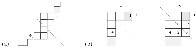
(a)

e_i

(b)

i

λ αλ

4 −4

4 2 −2 i

0 0

Figure 8. Examples (a), (b) for Lemma 6.6.

rowi′_{. But this cannot happen since that box is removable. (The argument in case} i′ _{=i+ 1 requires a slight modification.) The last claim is proved similarly.}

2

(6.5)Lemma. Fix δ and supposesδ(λ) =sδ(λ−ei)as before. Suppose λhas an

edge down labelled α, i.e. λ/αλ is aδ-pair; and letw be the product of commuting

reflections such thatwe_δ(λ) =e_δ(αλ), as in Lemma (4.11). Then (I)we_δ(λ−ei)

is dominant (i.e. w.(λ−ei)∈Λ);

(II)we_δ(λ−ei) =e_δ(α(λ−ei)).

Proof. Note thatoδ(λ−ei) =oδ(λ) by Lemma 6.4, soα(λ−ei) makes sense; and

oδ(α(λ−ei)) =oδ(αλ) (since both are equal to the formal set αoδ(λ)). Suppose

w.(λ−ei)isin Λ. Then it is in [λ−ei]δ by [8, Th.5.2], adjacent toαλwith the same

singularity, and by Lemma (6.4) (applied appropriately)oδ(w.(λ−ei)) =oδ(αλ). Thus it is enough to show (I).

We split into two cases. (A) Ifei intersectsλ/αλ thenπα(ei) is addable to αλ

as noted in (6.3). That ise_δ(αλ+πα(ei)) =we_δ(λ−ei) is dominant. (B) Ifeidoes

not intersectλ/αλthenwe_δ(λ−ei) is the same aswe_δ(λ) everywhere except in row i: we_δ(λ−ei) =we_δ(λ)−ei. Sinceλ−ei is dominant,λi> λi₊₁, but (αλ)_i=λi

in this case, and (αλ)i+1 ≤λi+1, so (αλ)i >(αλ)i+1, so αλ−ei is dominant, so

e_δ(αλ−ei) =we_δ(λ−ei) is dominant. 2

(6.6)Lemma.Fix δ and suppose sδ(λ) =sδ(λ−ei) as before. Suppose αλ/λ is

a δ-pair (i.e. α is an edge up from λ). Then there is a reflection group element

w such that w.λ = αλ (so w.αλ = λ) and w.(λ−ei) is dominant; whereupon

w.(λ−ei) =α(λ−ei).

Proof. As above it is enough to showw.(λ−ei)∈Λ. Given thatw.λis dominant, a

failureof dominance ofw.(λ−ei) must be either: (case A) a row with which row-i

is paired inw(j, say) is longer than row-(j−1) inw.(λ−ei); or (B) thei-th row itself is shorter than row-(i+ 1) inw.(λ−ei) (i.e. row-(i+ 1) intersects theδ-pair). We need to eliminate these.

Case (A): Suppose first that ei is ‘behind’ other than the last row of the skew. Then there is a box of the skew immediately to its right and one immediately below it. The π-rotation images of these are behind and above the image ofei, so

w.(λ−ei)∈Λ. On the other hand, supposeei is behind the last row of the skew. For example see Fig.8(a) (the boxπα(ei) is marked×). Herew.(λ−ei) is dominant unless the box aboveπα(ei) is missing fromλ. But if this is missing then this row and thei-row are a singular pair inλ−ei. Neither row can be in a singular pair in

λso this contradicts the hypothesis.

eigiven byπα(ei) is directly to the left of the skew, and we have a setup something like Fig.8(b) (the δ-balanced box is the box marked 4). If there is no box below the πα(ei) in λ then row-i is not in a singular pair inλ, and row-i and the row containing theπα(ei) are a singular pair inλ−ei, thussδ(λ)6=sδ(λ−ei) so we can exclude this. If there is a box below the πα(ei) in λthen this row and row-iare a singular pair inλ, and row-iand the row containing theπα(ei) are a singular pair inλ−ei. In this case, awwhich also has a factor acting on thei-th and undrawn row has the same effect onλas one which does not. Its effect onλ−ei is to restore the boxeiand to add a box in the undrawn row. Thisw.(λ−ei) is dominant since the added box is under a box added in the original skew. 2

Since the block graph Gδ(λ) is connected we may use Lemmas 6.5 and 6.6 to show:

(6.7)Theorem.If sδ(λ) =sδ(λ−ei)then Gδ(λ)is adjacent to Gδ(λ−ei). 2

(6.8) Lemma (6.4)(I) says that if the partitionsλ, λ−ei have the same singularity then they pass to the same point on the block graphGeven. That isfi(λ) =λ−ei

and so on. Thus forµ∈[λ]δ

hδ(λ)µ=hδ(λ−ei)fi(µ)

(6.9)Lemma.If sδ(λ) =sδ(λ−ei)then for all pairs (µ, fi(µ))∈[λ]δ×[λ−ei]δ

ProjλInd∆¯n(fi(µ)) = ¯∆n+1(µ)

Projfi(λ)Ind∆¯n(µ) = ¯∆n+1(fi(µ)) (11)

Proof. Note that the pair (µ, fi(µ)) are adjacent by Theorem 6.7. For any ν

Prop.3.14 gives Ind ¯∆(ν) =

+

_{+ +}

k∆(¯ ν−ek). Forν=fi(µ)

ad-jacent toµ, one of these summands is ¯∆(µ). Specifically either (i)µ=ν+el(some

l); or (ii)µ=ν−el (somel). In case (i) other summands are of formµ−el+ej,

µ−el−ek. By Prop.(4.5) the former are not in [µ]δ, and sincesδ(λ) =sδ(λ−ei),

Lemma (6.4)(II) excludes the latter. The other case is similar. 2

7. The Decomposition Theorem

(7.1) Theorem.For each δ ∈ Z _{the Brauer algebra ∆-decomposition matrix D}

overC_{is given by}

( ¯Pnδ(λ) : ¯∆nδ(µ)) =hδ(λ)µ or equivalently

¯

Pnδ(λ) =

+

δ n(µ).

(Recall we omit λ=∅ in case δ= 0.)

This data determines the Cartan decomposition matrixCfor any finitenby (3.16).

Proof. We prove for a fixed but arbitraryδ, working by induction onn. The base

cases aren= 0,1, which are trivial (andn= 2 forδ= 0, which is straightforward). We assume the theorem holds up to leveln−1, and considerλ⊢n. (For|λ|< n

(7.2) We call a removable box of largest magnitude charge (among those removable in the given skew) arim-end removable box. Examples are shown in Figure 2. The rim-end removable boxes (as labelled by charge) in the figure are (i) 22; (ii) -16; (iii) 8.

(7.3)Proposition.Fix δ. Pick α∈Γδ ,λ and letei be a rim-end removable box in

λ/αλ. Then

sδ(λ−ei) =

sδ(λ) + 1 if |λ/αλ|= 2

sδ(λ) otherwise

Proof: If|λ/αλ|= 2 the charges in the two boxes are (say)xand−x. Removingx

(from rowi) we get a row ending in chargex+ 2, giving (λ+ρδ)i=−x+2₂ +1₂ =

−x+1

2 . The row ending in−xhas (λ+ρδ)j =−

−x

2 +

1 2 =

x+1

2 thus these two rows are now a singular pair.

For|λ/αλ| 6= 2 there is a unique rim-end removable box. The caseλ/αλ= (22₎ is elementary. We split the remainder into two cases. If the upper end of a rim in

λ/αλends in a row of length greater than 1 then the removable box is at the upper end. Write−xfor its charge andi for its row. (Cf. the upper rim in Figure 2(ii), which ends in−x=−16.) Note that in this case there cannot be a row inλending in a box with chargex+ 2 orx. Note that a pair of rows is singular if the sum of charges in their end boxes is 2. It follows that neither the i-th row of λnor that of λ−ei is in a singular pair. Thus λ, λ−ei have the same set of singular pairs. (Indeed we remain in the same facet.)

If the lower end of a rim in λ/αλ ends in a column of length greater than 1 then the removable box is at the lower end. Writexfor its charge andifor its row. (Cf. the lower rim in Figure 2(i), which ends in x= 22; and Fig.2(iii) which ends in

x= 8.) Note that in this case there is a row inλending in a box with charge−x, and one with −x+ 2. It follows that both thei-th row of λand that ofλ−ei is in a singular pair (albeit each with a different partner). Thusλ−ei has a different set of singular pairs, but the samenumberof pairs: sδ(λ−ei) =sδ(λ). 2

(7.4) Proposition. Fix δ. For λ ∈ Λ pick α ∈ Γδ ,λ and let ei be a rim-end

removable box in λ/αλ. In case |λ/αλ| 6= 2

(i) the∆-decomposition data for P¯(λ)is the ‘translate’of that for P¯(λ−ei):

( ¯P(λ) : ¯∆(µ)) = ( ¯P(λ−ei) : ¯∆(fi(µ))) ∀µ∈[λ]δ

(ii) This verifies the inductive step for the main theorem in such cases. That is, hδ(λ)∼=hδ(λ−ei).

Proof: By Proposition 3.18 the ‘translation’ ProjλInd ¯P(λ−ei) = P¯(λ)⊕Q

withQ= ProjλQsome projective, possibly zero. In case|λ/αλ| 6= 2 each standard

module occuring in ¯P(λ−ei) induces precisely one standard module after projection onto the block of λ, by Lemma 6.9 (noting Proposition 7.3). More specifically, suppose ¯∆(ν(1)),∆(¯ ν(2)), ...,∆(¯ ν(l)) is a ∆-filtration series for ¯P(λ−ei) (i.e. ¯P(λ−

ei)≃//j∆(¯ ν(j))). Then by (6.2) there is a sequenceµ(1), µ(2), ...such thatν(j) =

fi(µ(j)); and (using Prop.3.14(i), 3.16 and exactness of Res−and Projλ−)

¯

P(λ)⊕Q= ProjλInd ¯P(λ−ei) ≃ //jProjλInd ¯∆(fi(µ(j))) = //j ∆(¯ µ(j))

On inducing again and projecting back to the block ofλ−ei, by (11) we have

That is, each standard module occuring in ( ¯P(λ)⊕Q) induces precisely one stan-dard module after projection onto the block of λ−ei. It follows that this second ‘translation’ may be identified with ¯P(λ−ei) again. Since this is indecomposable,

thefirsttranslation cannot be split, and hence is precisely ¯P(λ) — with the same

decomposition pattern. For the last part use (6.8). 2

(7.5)Proposition.Fix δ. Pick α∈Γδ ,λ and letei be a rim-end removable box in

λ/αλ. In case |λ/αλ|= 2

(I)bδ(λ) = ˆαbδ(λ−ei),bδ(αλ) = ˇαbδ(λ−ei).

(II) If( ¯P(λ−ei) : ¯∆(ν)) =hδ(λ−ei)ν (allν) then( ¯P(λ) : ¯∆(µ)) =hδ(λ)µ (allµ).

Proof: (I) As shown in the proof of Prop. 7.3, removingei from λmakes that row

part of a singular pair with the row containing the box with opposite charge. Thus a pair which contributed an 01 sequence inbδ(λ) does not contribute tobδ(λ−ei)

— i.e. bδ(λ) = ˆβbδ(λ−ei) for someβ. It remains to confirm the position of the modification. For somex≥0 and somei′ _{we have}

e_δ(λ) = (λ₁−δ

2, ...,

i−th

z }| {

x+ 1 , ...,

i′_−th

z}|{

−x , ...)

e_δ(λ−ei) = (λ₁−δ

2, ..., x , ..., −x , ...)

e_δ(αλ) =e_δ(λ−ei−ei′) = (λ1−δ₂, ..., x , ..., −x−1 , ...) Altogether thei, i′_{-pair contribute an 01 (resp.10) in b}

δ(λ) (resp. bδ(αλ)). Since

theαaction on λmanifests (by definition) as 10↔01 in theα, α+ 1 position of

bδ(λ) we see that β=α.

(II) Applying Projλ−to Proposition 3.14(ii) here we get a short exact sequence

0→∆(¯ λ−ei−ei′)→Proj_λInd ¯∆(λ−ei)→∆(¯ λ)→0 (12)

(non-split, by [7, Lemma 4.10]). Translating ¯P(λ−ei) away from and then back to λ−ei therefore produces a projective whose dominating content is two copies of ¯∆(λ−ei) (one from each of the factors in (12)). Hence, by (3.17), Projλ−eiInd (ProjλInd ¯P(λ−ei)) = P¯(λ−ei)⊕P¯(λ−ei). It follows that

ProjλInd ¯P(λ−ei) = P¯(λ). Now assume ( ¯P(λ−ei) : ¯∆(−)) = hδ(λ−ei). It

remains to show that (ProjλInd ¯P(λ−ei) : ¯∆(−)) =hδ(λ).

For each ¯∆(µ) in ¯P(λ−ei) one sees readily that ProjλInd ¯∆(µ) = ¯∆(ˆαµ)+ ¯∆(ˇαµ).

That the collection thus engendered overall is hδ(λ) now follows directly from (I) and Equation(9). Indeed we have (non-split [7, Lemma 4.10]) 0 → ∆(ˇ¯ αµ) → ProjλInd ¯∆(µ)→∆(ˆ¯ αµ)→0.2

Proposition 7.5 completes the cases for the main inductive step, establishing the Theorem. 2

(7.6) Example for Proposition 7.5:δ= 1, computing forλ= 4422 viaλ−e2= 4322. We have e₁(4322) = (7/2,3/2,−1/2,−3/2, ...) so o₁(4322) = toggle({2}) ={1,2}.

By the inductive hypothesis we have

( ¯P(4322) : ¯∆(−)) = h1(4322)− =

4322

D D D D D D

221 ∼ =

12

12??? ? ? ?

∅ ∼ =

01

B B B B B B

10

representation. Note that we have reverted to the untoggled form at the last since we will be inserting an 01 subsequence (removing the need for the toggle) at the next step. Translating off the wall we get 4322+221→(4422+4321)+(321+22). In binary this corresponds to 01→0∗∗1→0101+0011 and 10→1∗∗0→1100+1010. These four sequences therefore encode the content ofP4422.

The Theorem is verified in this case, since:

h1(4422) =

4422

ttt HHH

4321

J J

J 321

vvv

22

∼ =

34 23

xxx ₁₄FFF

24

F F

F 13

xxx

12

∼ =

0011

ttt HHH

0101

J J

J 101

vvv

11

Note how the insertion of a binary pair in the α position, and action of α on that pair, transforms h1(4322) to produce h1(4422). The effect is (i) to extend the hypercube by a new generating direction (labelled by α); (ii) the generating edge inherited fromh1(4322) changes label from 12 to 14 due to the bump (which illustrates how such non-Geven edge labels arise in this construction).

8. On parabolic Kazhdan–Lusztig polynomials

Associated to each Coxeter system (W′_{, S}′_{) and parabolic (W, S), acting as}

re-flection groups on space V, is an arrayP =P(W′_{/W) of Kazhdan–Lusztig}

poly-nomials — one for each ordered pair of alcoves. (Deodhar’s recursive formula [11] computes these polynomials in principle. However it generally tells us little about them in practice.) These polynomials play analogous roles to ha in certain cases in representation theory (see [22, 20] and references therein). Finally, then, we explain where the combinatorialideafor the form ofha comes from, by computing

P(D/D+).

8.1. The recursion for arrayP(W′_{/W). Let (W}′_{, S}′_{) be a Coxeter system,}

con-taining (W, S) as a parabolic subsystem. LetGa be the equivalent ofGalc in this case, and write (A+_{, <) for the poset defined by this acyclic digraph. The array}

P = P(W′_{/W) is a (generally semiinfinite) lower unitriangular matrix, with row}

and column positions indexed by A+_{. Write P = (pAB)}

A,B∈A+. It is natural to

organise this data into rows (although it is also of interest to organise into columns). The rows are thus of finite support.

The recursion for rows ofP above the root in the poset order is as follows (see [22] for equivalent constructions). To compute the rowpAwe first compute another polynomial for each alcoveD,p′

AD, also denotedp′A(D) as follows. (Actuallyp′A(D)

can depend on the choice made next in the computation, butpA does not and we supress this dependence in notation.)

Pick an edge (B, A) inGa ending atA(sopB is known). For each alcoveD let Γ±D

be the set of alcovesD′ ofGa such that (D′, D) (resp. (D, D′)) is an edge in the orbit of the edge (B, A). (By the Cayley property (4.20) we can express (B, A) = (B, Bs),s∈S′_{, whereupon any suchD}′ _{must obey (D}′_{, D) = (D}′_{, D}′_{s) = (Ds, D)}

(respectively (D, D′_{) = (D, Ds)).) Then}

p′A(D) =

X

D′∈Γ+

D

(v−1pB(D) +pB(D′)) + X

D′∈Γ−

D

(vpB(D) +pB(D′)) (13)