Design of High-performance Networked Real-time Control Systems
Peng Wen
1, Jiannong Cao and Yan Li
2 31Faculty of Engineering and Surveying
3Department of Mathematics and Computing University of Southern Queensland, Australia
2Internet and Mobile Compute Lab Department of Computing
Hong Kong Polytechnic University, Hong Kong
[email protected]; [email protected]; [email protected]
Abstract: The performance of a networked control system (NCS) is affected directly and indirectly by time delays generated in network communication. This paper addresses these time delays, their effects on system performance, and the measures taken in an NCS design. For a time delay which is random but less than one sampling interval T, we model the system as a time-invariant control system with constant time delay T. For a time delay which is random and greater than one sampling interval T, we consider the system as a control system with packet drop and model it as a jump linear control system. Based on the above models, we propose a systematic method to improve the control system quality of performance by choosing a proper sampling interval to reduce data transmission, optimally scheduling to minimize packet loss and optimizing controller design in case of packet loss. The simulation results in lab experiments demonstrate that the design method results in high performance in networked real-time control system.
Key words: Real-time system, networked control system, time delay, packet drop, optimal control.
Design of high-performance networked real-time
Wen, Peng and Cao, Jiannong and Li, Yan (2007)
control systems. IET Control Theory and Applications, 1 (5). pp. 1329-1335. ISSN 1751-8652
Introduction
Networked control systems are real-time systems where sensor and actuator data are transmitted through a shared or switched communication networks. The use of a data network in a control system path has several advantages such as re-configurability, low installation cost, and easy maintenance. It is also well suited for large geographically distributed systems. Wireless communication is playing an increasing important role in such a networked control system. Transmitting sensor measurement and control commands over wireless links allows rapid deployment, flexible installation, fully mobile operation and prevents the cable wear and tear problem in industrial environment. However, the introduction of a communication network into a networked control system can also degrade overall control system performance through quantization errors, transmission time delays and dropped measurements.
Building a networked control system over network links is a challenging task. First, the communication channel imposes a fundamental limit on the quality of service (QoS) of networks, and the random delays and packet losses are inevitable. The time delays caused by network communication are quite different from the usual control system time delays. They are inherently dynamic and cannot be anticipated before the systems are developed. Depending on the magnitude of network time delays relative to the sampling interval, their effects on the performance of a control system are originated from either a packet delay or packet loss. To be more precise, let τ and T denote the communication delay and the sampling interval, respectively. A delay problem results when
0
<
τ
<
T
, or whenτ
is a fixed value. The loss problem occurs whenτ
≥
T
as a delayed measurement is almost useless to a real-time control system and could be dropped to save limited bandwidth. The former represents the undesirable effects caused by a nonzero network time delay, while the latter represents the case of no update measurement or control output for one or more sampling intervals.This paper addresses the problems in high-performance networked control system design, and focuses on how to overcome the time delays and packet drop caused by communication networks. We start with identifying the time delay and packet loss problems over a communication network. Then, we analyze how the time delay affects control system performance and propose to minimize data transmission by choosing a proper sampling period. For the packet loss problem, we model it as a task failure of a periodic real-time system. Then we propose a schedule method to minimize the packet loss. In the case of packet loss, we provide a method to optimize the controller design. These methods and measures are tested in simulation and lab experiment.
The rest of the paper is organized as follows. Section 2 reviews the existing work. Section 3 discusses the network delay and its impact on system performance, and proposes a method to minimize data communication by selecting a proper sampling interval. Section 4 addresses the packet loss problem by proposing prevention methods and the optimal control based on unreliable data links. Simulations and experiment results are given in Section 5. The conclusion is drawn in Section 6.
2. Previous work
Network induced time delays can be constant, varying, or even random depending on the medium access control (MAC) protocol of a network. Networks for control purpose using CSMA protocols include DeviceNet and Ethernet [1-2]. A node on a carrier sense multiple access (CSMA) network monitors the network before each transmission. When the network is idle, it begins transmission immediately. Otherwise it waits until the network is not busy. When two or more nodes try to transmit simultaneously, a collision occurs. The way to resolve the collision is protocol dependent. DeviceNet, which is a controller area network (CAN), uses CSMA with a bitwise arbitration (CSMA/BA) protocol. Since CAN messages are prioritized, the message with the highest priority is transmitted without interruption when a collision occurs, and transmission of the lower priority message is terminated and will be retried when the network is idle. Ethernet employs a CSMA with collision detection (CSMA/CD) protocol. When there is a collision, all of the affected nodes will be back off, wait for a random number of time slots, and retransmit. Packets on these types of networks are affected by random delays, and the worst-case transmission time of packets is unbounded. Therefore, CSMA networks are generally considered nondeterministic. However, if network messages are prioritized, higher priority messages have a better chance of timely transmission.
the communication in the networks, packet transmission time delays occur while waiting for the token or time slot. Transmission delays can be made both bounded and constant by transmitting packets periodically [3].
Halevi and Ray [4] studied a clock driven controller with mis-synchronization between plant and controller. The system was represented by an augmented state vector that consists of past values of the plant input and output, in addition to the current state vectors of the plant and controller. This resulted in a finite-dimensional, time-varying discrete-time model. They also took message dropping into consideration. Nilsson [5] analysed NCSs in the discrete-time domain. He further modelled the network delays as constant, independently random, and random but governed by an underlying Markov chain. From there, he solved the Linear Quadratic Gaussian (LQG) optimal control problem for the various delay models. He also pointed out the importance of time-stamping messages, which allowed the history of the system to be known. Walsh et al. [6] considered a continuous plant and a continuous controller. The control network, shared by other nodes, was only inserted between the sensor nodes and the controller. They introduced the notion of maximum allowable transfer interval, denoted by τ, which supposed that successive sensor messages were separated by at most τ seconds. Their goal was to find that value of τ for which the desired performance (stability) of an NCS was guaranteed to be preserved.
Approaches for compensation for data loss over network links have also been proposed, among others, by Nilsson [5] and by Ling and Lemmon [7], who posed the problem of optimal compensator design for the case when data loss was independent and identically distributed (iid) as a nonlinear optimization. A sub-optimal estimator and regulator to minimize a quadratic cost were proposed by Azimi Sadjadi [8] and this approach was extended by Imer et al. in [9] and Sinopoli et al. in [10-11]. However, most of the work aimed at designing a packet loss compensator. The compensator used the successfully transmitted packets to come up with an estimate of the plant state. This estimate is then used by the controller. Gupta et al. realized that sensors and actuators equipped with wireless or network communication capabilities would likely have some computational power. They took these computational capabilities into consideration and extended the above result further. They introduced an encoder at the sensor end. The compensator then became a decoder for the information being transmitted over the unreliable link. The control, the encoder and the decoder were jointly designed to solve the packet loss problem and to achieve an LQG optimal control.
3. NCS performance with time delay
In a NCS, information among distributed sensors, controllers and actuators are shared over a communication network. Communication over shared network causes time delays in various sections of a NCS. These time delays cannot be neglected, especially when the time constant of the controlled plant is short and the order of the plant model is high [1]. They may affect network QoS and degrade control quality of performance (QoP).
In a NCS, message transmission delay can be broken into two parts: device delay and network delay. The device delay includes the time delay at the source and the destination nodes. The time delay at the source node includes the pre-processing time, Tpre, and the waiting time, Twait. The time delay at the destination node is only the
post-processing time, Tpost. The network time delay includes the total transmission time, Ttx, of a message and the
propagation delay of the network. The total time delay can be expressed as the follow [12].
Tdelay=Tpre +Twait +Ttx +Tpost (1)
The pre-processing time at the source node is the time needed to acquire data from the external environment and encode it into the appropriate network data format. This time depends on the device software and hardware characteristics. A message may spend time in a queue at the sender buffer before been transmitted or discarded. Depending on the amount of data the source node must send, the transmission protocol and the traffic on the network, the waiting time may be significant. Most of the time, the waiting time is random. The transmission time is the most deterministic parameter in a network system. The post-processing time is negligible in an NCS comparing to other time delays.
3.1. NCS Model with a short or constant time delay
...}
2
,
1
,
0
,
{
),
(
)
(
)
(
)
(
]
1
,
[
),
(
)
(
)
(
=
+
∈
−
−
=
=
+
+
+
∈
+
=
+
KX
t
t
k
k
t
u
t
CX
t
Y
k
k
t
t
Bu
t
AX
t
X
k k k kτ
τ
τ
τ
&
(2) kk
+
τ
where u(t+) is piecewise continuous and only changes value at . By sampling the system with period T
we obtain
.
)
(
,
)
(
,
where
)
(
)
(
),
1
(
)
(
)
(
)
(
)
(
)
1
(
1 0 0 1 0∫
∫
− −=
Γ
=
Γ
=
Φ
=
+
Γ
+
Γ
+
Φ
=
+
T T As k T As k AT k k k kBds
e
Bds
e
e
k
CX
k
Y
k
u
k
u
k
X
k
X
τ ττ
τ
τ
τ
(3)Defining Z(k)=[XT(k),u (k-1)]T T as the augmented state vector, the augment closed loop system is
.
0
)
(
)
(
)
(
where
)
(
)
(
)
1
(
1 0 ~ ~⎥
⎦
⎤
⎢
⎣
⎡
−
Γ
Γ
−
Φ
=
Φ
Φ
=
+
K
K
k
k
Z
k
k
Z
k kτ
τ
(4)In the case that the delay is less than one sampling interval T, we can estimate the maximum delay as T. The NCS system becomes a time invariant one. This type of systems can be analyzed using well-developed techniques.
When the delays can be longer than one sampling interval T, in this case the delayed packets will be dropped and the situation will be considered in the packet loss section. However, in a special case where (m-1) <τk<m for
all k is a constant, one control sample is received every sample period for k>m. In this case, the analysis follows that in [13], resulting in
T T T T k k k k
k
u
m
k
u
k
X
k
Z
m
K
I
)]
1
(
,
),
(
),
(
[
)
(
)
1
(
where
0
0
0
0
0
0
0
)
(
)
(
' ' 0 ' 1 ~
−
−
=
−
−
=
⎥
⎥
⎥
⎥
⎥
⎦
⎤
⎢
⎢
⎢
⎢
⎢
⎣
⎡
−
Γ
Γ
Φ
=
Φ
L
L
M
O
M
M
M
L
L
τ
τ
τ
τ
(5)Even in this simplest case, the next question is how long the time delay in an NCS system can tolerate before it becomes unstable.
To guarantee system stability and the performance, two control measures can be used: phase margin and control system bandwidth [3]. Phase margin is the change in open-loop phase shift required at unity gain to make the closed-loop system unstable. This margin can be obtained from system Bode plots or Nyquist plot. The primary effect of time delay is additional phase lag in system frequency response. In other words, the time delay does not affect the magnitude frequency response curve, but it does subtract a linearly increasing phase shift, ωT, from the phase frequency response. This can be seen in the following equation:
{
(
)
}
)
(
)
(
)
(
'
j
ω
e
ωG
j
ω
G
j
ω
ω
T
G
j
ω
G
=
−j T=
∠
−
+
∠
(6)
where G’(jω) is the system frequency response with time delay T, and G(jω) is the system frequency response without any time delay.
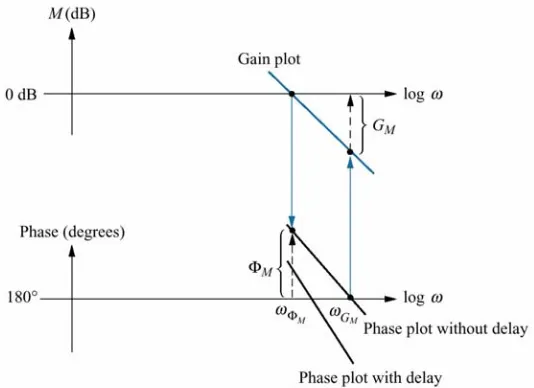
(Figure 1 goes here)
[image:5.595.71.301.399.467.2]The typical effect of adding time delay can also be seen in Figure 1. Assume that the gain and phase margin as well as the gain- and phase-margin frequencies shown in the figure apply to the system without delay. From the figure, we see that the reduction in phase shift caused by the time delay reduces the phase margin. Using a second order approximation, this reduction in phase margin yields a reduced damping ratio for the closed-loop system and a more oscillatory response. The reduction of phase also leads to a reduced gain margin frequency. A reduced gain margin frequency not only reduces the gain margin but also reduce the system bandwidth.
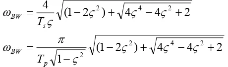
System bandwidth, ωBW, is defined in frequency domain as the frequency at which the magnitude response curve
is 3dB down from its value at zero frequency. In time domain it is interpreted as the maximum frequency at which the output of a system will track an input sinusoid in a satisfactory manner. Using a second order approximation, the system bandwidth can be related to system transient response in settling time and pick time in the following equations.
2
4
4
)
2
1
(
1
2
4
4
)
2
1
(
4
2 4 2
2
2 4 2
+
−
+
−
−
=
+
−
+
−
=
ς
ς
ς
ς
π
ω
ς
ς
ς
ς
ω
p BW
s BW
T
T
(7) where Tp, Tsandζ are system pick time, settling time and damping factor.
All the signals in an NCS system have to be discretized. Assume the discretization is implemented using A/D converters (ADCs). The ADCs sample signals and hold them until the next sampling instant comes. This procedure automatically generates one sampling period time delay, Ts, for all the sampled signals. This means
that there is a phase lag
φ
s=
ω
T
sdue to discretization. The phase lag due to time delay caused by network communication isφ
d=
ω
T
d. The total phase lag due to discretization and communication time delays can be expressed as follows:d s d
s
φ
ω
T
ω
T
φ
φ
=
+
=
+
(8)The maximum phase lag that an NCS system can tolerate with stability is its phase margin φM, we then have
)
(
s dd s d s
M
=
φ
+
φ
=
ω
T
+
ω
T
=
ω
T
+
T
φ
(9)The maximum time delay Td can be determined as
s M
d
T
T
=
−
ω
φ
(10)
BW
ω
s BD M
d
T
T
=
−
ω
φ
(11)
Td is the maximum time delay an NCS system can tolerate before it becomes unstable.
4. Model and optimal control based on packet loss
When time delay is irregular and longer than one sampling interval, the delayed packet is dropped. Packet loss is, therefore, another direct factor in NCS system performance degradation. Any improvement in packet loss can directly improve system performance.
4.1. NCS sampling period selection
Sampling is a major process in a control system. The sampling interval determines how frequently the sensors, controllers and actuator exchange their data through the shared networks. The sampling rate, therefore, must be chosen carefully by not only satisfying the Shannon’s sampling theorem, but also minimizing the data transmission. A higher sampling rate can improve performance and achieve higher stiffness (or disturbance rejection property). Increasing the sampling frequency, however, puts more data into the communication links, causes longer time delay and packet loss, and degrades system performance. Therefore, there is an upper bound for the sampling period. That means the network traffic is saturated in this sampling period. Any sampling period smaller than that would cause longer time delay and packets losses, and degrades the performance in an NCS system. The lower sampling period bound can be estimated using schedulability conditions. As these period tasks in an NCS system might be scheduled using Rate-Monotonic (RM) and Early-Deadline-First (EDF) algorithm, both schedulability conditions of RM and EDF should be met [3]. That is
)
n(
T
T
)
n(
T
T
,
T
T
T
s /n d/n d s d s s
1
2
1
2
1
max
)
min(
1 1−
+
=
⎟⎟
⎠
⎞
⎜⎜
⎝
⎛
−
+
+
=
(12)
where Ts is sampling interval and Td is network time delay.
For an NCS system, the numbers of period tasks are case dependent and sometimes are dynamic. A better estimation for this is
69
.
0
69
.
0
)
min(
s d ds
T
T
T
T
=
+
≅
(13)
where 0.69 is the maximum ratio of utilization to meet the sufficient schedulability for infinite period tasks [3], and Ts can be ignored as it is too small comparing with Td. When the device processing time and other delays are
considered, however, the lower sampling period bound would be increased further. A proper sampling period of an NCS should be below this bound.
4.2. Periodic task scheduling
For a real-time networked control system, most processes are periodic. While some of these periodic processes are completed locally, they need to share their data among sensors, controllers and actuators through networks. To use the shared networks efficiently, we need to schedule these data communications properly. If we consider each of these data transmissions as a periodic task, then they can be modelled as time periodic tasks in real-time computing system.
time, called the notification time. On or before the notice time if alternates are not scheduled, they can not be completed in time.
Applying this approach to our data transmission tasks, we get two versions for each of our n data transmission tasks. These tasks form a real-time periodic system. For this real-time periodic task system, all the alternates are scheduled using a fixed priority-driven scheduling algorithm to reserve time intervals as late as possible in a planning cycle before runtime. At runtime, if there are primaries pending during the time intervals that are not reserved by alternates, the scheduler chooses the primaries to execute. The primaries can be scheduled by an online scheduling algorithm, such as a (fixed or dynamic) priority-driven pre-emptive scheduling scheme with the RM or EDF priority assignment. A primary may fail at any time during its execution or take too long to complete. If a primary fails, its corresponding alternate must be executed. Moreover, when the notification time of an alternate Aij is reached, yet its corresponding primary Pij has not been completed or has failed, Aij is
activated. That is, pre-empting the execution of any primary, including Pij, or other lower-priority alternates. For
the primary Pij, if it has not been finished, it will be aborted since its alternate, Aij, is chosen to be executed. If
the primary is not Pij, it will be suspended and resumed later. Every alternate, if activated on or after its
notification time, has higher priority than all primaries and the activated alternates are executed according to their priorities assigned by the offline fixed-priority algorithm.
In calculating the notification times, we consider only the alternates, Aijs. We use ai as the computing time of τi and use a fixed–priority algorithm to construct a schedule (for example, by using the slack interval method to calculate it backward from time T to time 0, and find the finish time v ijof Aij in the schedule, for each n ≥ i ≥1
and ni ≥ j ≥1 (ni is the job number). We then use vij as the notification time of Aij at runtime. That is, the
notification times are the finish times of the alternates if they are scheduled by a fixed-priority algorithm backward from time T. Note that the notification times force the alternates to be scheduled as late as possible and, hence, the scheduling algorithm leaves the largest possible room for executing the primaries before executing the alternates.
The objective of our scheduling algorithm is to guarantee either the primary or alternate version of each job to be successfully completed before its corresponding deadline while trying to complete as many primaries as possible. This can efficiently reduce the packet loss by deadline expiring.
4.3. NCS system modeling and optimization
If any communication task is not completed by its deadline, it has to be discarded as delayed measurements or control actions are useless for most real-time control systems. Many approaches have been proposed to compensate for the data drop or packet loss in NCS system. The simplest one is to reuse the previous packet. In this case, the received packets are considered as individuals. However, the data from a controlled plant is closely related to each other. One packet loss is only a piece of a whole data set from a plant. If we can consider this set of data as a whole picture, then the lost packet might be estimated from the previous packets. That will provide an opportunity for us to minimize the impact of packet loss on system performance. Here we propose to use the successfully transmitted packets to come up with an estimate of the plant state. This estimate is then used to design an optimal control.
Consider a discrete time linear system evolving according to
)
(
)
(
)
(
)
1
(
k
AX
k
Bu
k
W
k
X
+
=
+
+
(14)where X(k) is the plant state vector, u(k) is the control input vector and W(k) is the plant noise assumed to be white, Gaussian, and zero mean with covariance matrix Qw. Some of the plant states are measured directly and
some are measured and transmitted as packets through shared networks. There are no packet losses for the directly measured data. However, the data measured through networks could be lost randomly. That is
[
]
⎥
⎦
⎤
⎢
⎣
⎡
+
⎥
⎦
⎤
⎢
⎣
⎡
=
⎥
⎦
⎤
⎢
⎣
⎡
)
(
)
(
)
(
)
(
)
(
)
(
2 1
2 1 2 1 2
1
k
V
k
V
k
X
k
X
C
C
k
Y
k
Y
(15)
where Y1(k) are measured data through networks andY2(k) are directly measured data. The measurement noise
are assumed white, zero mean, Gaussian and independent of the plant noise W(k). Note that
if we let C
⎥
⎦
⎤
⎢
⎣
⎡
=
)
(
)
(
)
(
2 1
k
V
k
V
k
V
connected through networks. If we let C1=0, the above system would be reduced to a normal control system
without including any networks.
To simplify our discussion, we consider a special case where there are two sensors. Each is connected through network link L1 and L2 respectively. However, while L1 drops packets randomly, L2 transmits all packets
successfully. Then we can apply the results in [12] to our system. The process can be summarized as follows.
Denote by si(k) the finite vector transmitted from the sensor i (i=1,2) to the controller at time step k. By
causality, si(k) can depend on yi(0), y (1),…, y (k); i.e.i i ,
))
(
,
),
1
(
),
0
(
(
)
(
k
f
y
y
y
k
s
i i i ik i
L
=
. (16)The information set, I(k)available to the controller at time k is the union of two sets I1(k) and I2(k) defined by
}
0
|
)
(
{
)
(
}
s.t.
,
|
)
(
{
)
(
2 2 1 1k
j
j
s
k
I
received
j
j
s
k
I
jL
=
∀
=
=
∀
=
η
(17)Also denoted by
t
1(
k
)
≤
k
the last time step at which a packet was delivered over link L1. That is} " " | max{ ) (
1 k j k received
t = ≤ ηj = . The maximal information set, at time step k is then the union of I max , 1 k
I
2k and the set defined by . The maximal information set is the largest set of
output measurements on which the control at time step k can depend. In general, the set of output measurements on which the control depends will be less than this set, since earlier packets, and hence measurements, may have been dropped. Without loss of generality, we will only consider controllers of the form . We denote the set of control laws allowed by U. We shall assume perfect knowledge of the system parameters A, B,
C, Q
max , 1
k
I
{
(
)
|
0
1(
)}
1 max ,
1
y
j
j
t
k
I
k=
≤
≤
)
,
(
)
(
k
u
I
k
u
=
kand Q
w v at the controller. Moreover we assume that the controller has the access to the previous control
signals u(0), u(1),…,u(k-1) while calculating the control u(k) at time step k. Finally, we can pose the packets based on LQG problem as:
)]
1
(
)
1
(
)
1
(
)
1
(
)
1
(
)
(
)
(
(
[
)
,
,
(
min
0 ,+
+
+
+
+
+
+
=
∑
= ∈ ∈K
X
K
P
k
X
k
X
R
k
X
k
u
Q
k
u
E
P
f
u
J
C T K k C T C T i K F f U u i (18)Here K is the horizon on which the plant is operated and the expectation is taken over the uncorrelated variables X(0), {Wk} and {Vk}. The parameters with superscript C are for the controller. Note that the cost function, Jk,
above depends on the random packet drop sequence P.
We aim to choose u(k) to minimize for given . The standard optimal LQG control technique gives us,
s
f
j)
,
,
(
u
f
P
J
j k)
(
)
(
)
(
1 1, _
K
AX
P
B
R
K
u
c K T C Ke − +
−
=
. (19)In the absence of the packet based link, the controller could simply use the standard optimal form. However, this control law does not lie in the set of allowable solutions U because it is not realizable for any non-trivial packet dropping sequence. Instead, we will calculate u(K) based on the information set IK and choose it to minimize JK.
The control problem thus reduces to an optimal estimation problem. Based on the information set I(K) at time K, and the previous controls (u(0), u(1), …,u(K-1), we denote the least mean square (LMS) estimate of a random
variable u(K) as
(
)
. Then we can write the optimal control at time step K as^
(20)
))
(
|
(
)
(
))
(
|
(
)
(
^
1 1
, ^
K
I
K
X
A
P
B
R
K
I
K
u
K
u
c K T C
K
e − +
−
=
=
Thus, we only need to find out the LMS estimate of X(K), given the information I(K) available to the controller. The details of how to estimate X(K) is given in [12].
)) ( | ( ^
K I K X
5. Examples and experimental testing
These approaches or methods proposed in the previous sections can be applied to NCS system design directly. The simulation and experimental testing are presented in this section.
5.1.Communication task scheduling
To verify our communication task scheduling algorithm, a simulation is carried out. The task set used in the simulation is τ=[τ1 , τ2 , τ3, τ4] with task (Ti, pi, a ), i=1, 2, 3i and 4. Here Ti is the task period, pi primary
transmitting time and ai the alternate transmitting time. We have τ1=(15, 4, 2), τ2=(24, 5, 3), τ3=(40, 10, 5), and
τ4=(160, 30, 15). Let the planning cycle, T, be the least common multiple (LCM) of τ1, τ2, τ3, τ4. Then the
planning cycle T is T=LCM(T1, T2, T3, T4)=LCM(15, 24, 40, 160)=2400. We test this algorithm for different
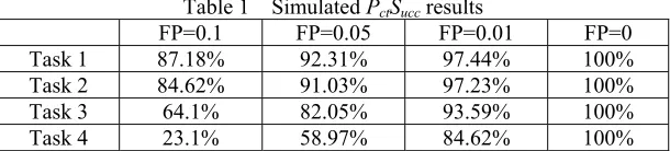
primary failure rates. The simulation results in the table below are presented by the metrics, PctSucc, which
[image:9.595.146.451.347.416.2]indicates the percentage of successfully completed primaries for each task.
Table 1 Simulated PctSucc results
FP=0.1 FP=0.05 FP=0.01 FP=0
Task 1 87.18% 92.31% 97.44% 100%
Task 2 84.62% 91.03% 97.23% 100%
Task 3 64.1% 82.05% 93.59% 100%
Task 4 23.1% 58.97% 84.62% 100%
In the above table, the metrics: PctSucc is calculated as follows. Suppose FP (failure probability) is 0.1 and there
are 20 jobs, then there are two primary failures because of FP × 20=0.1× 20=2, and 18 of the 20 jobs will complete successfully. If the actual schedule accommodates only nine successful primaries, then PctSucc=9/18=50%. That is, PctSucc is the percentage of actual successful primaries among the maximum possible
successful primaries. It represents how many subsequent primaries are affected by the early failures and how well the scheduling algorithm deals with early primary failures.
The simulation results in the above table indicate that the lower priority task suffers failure more significantly. For example, for FP=0.1, the percentage of successful primaries for Task 4 degraded to only 23.1%, while that of Task 1 is greater than 87.18%. The primary of Task 4 gets less of a chance to be executed because of its lower priority.
In this scheduling algorithm, however, as the alternate is guaranteed, the packet loss caused by deadline expiring has been avoided successfully no matter the primary or the alternate is completed.
5.2. Experimental testing
Incitec Limited is a large chemical manufacturing company with facilities located Australia wide. It is Australia’s largest fertilizer manufacturer, producing products such as ammonia, ammonium nitrate and urea. It has two main manufacturing sites, one at Gibson Island in Brisbane and the other at Kooragang Island in Newcastle. To maintain competitive the manufacturer has undergone a number of upgrades to maximise capacity and efficiency with minimum personnel or equipment cost. We propose to monitor and control this mixed large system through Internet which is available almost everywhere.
This network based real-time monitoring and control system can be modelled as a real-time periodic task system. In this system, there are six periodic tasks. They are
• Data acquisition
• Signal conditioning
• Control algorithm computation
• System data updating
• Display
Data acquisition is a task that deals with IO interfaces. It is the busiest task among the all. It is driven by a real-time clock interrupt and activated by AD conversion interrupts. A flag signal will be set up by the data acquisition task to inform the signal conditioning task, once a scan is completed. The signal conditioning task applies a digital filter to these measured data and provides noise-free signals to a control algorithm. The control algorithm calculation task carries out the calculation based on the noise-free input signals, controller parameters, system states and other constraints. The outcomes from this task are a sequence of control signals. These control signals are outputted to actuators immediately to keep the computation time delay to the minimum. After that, the system data updating progress will be activated. It will renew the system states using measured data, record the control signals and adjust parameters if necessary. Finally, the display task will refresh all the displayed information in the local control board. The communication task will run periodically to upload system information for storage or display purposes through the Internet.
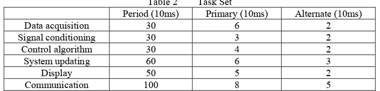
[image:10.595.106.490.284.376.2]As this is a distributed system, there are many computers and micro-controllers included. It is hard to do the scheduling as these tasks are executed in parallel by different processors. We have to normalise these transmission times and task periods into an equivalent transmission time and task periods. The outcomes for this normalisation are listed in the table below:
Table 2 Task Set
Period (10ms) Primary (10ms) Alternate (10ms)
Data acquisition 30 6 2
Signal conditioning 30 3 2
Control algorithm 30 4 2
System updating 60 6 3
Display 50 5 2
Communication 100 8 5
An inspection to the above table, we can see that the communication link utilization factor for this system is
. 713 . 0 100
8 50
5 60
6 30
4 30
3 30
6 )
( 1
= + + + + + = =
∑
= n
i i i
T e
U
τ
The least upper bound for it is. Obviously, 735
. 0 ) 1 2 ( 6 ) 1 2
( 1/n− = 1/6− =
n U(τ)=0.713<0.735, the system is then schedulable both by RM and EDF.
A prototype system is set up in our control lab through the Internet. There are two industrial PC computers in this prototype system. One computer is supposed to be located in the workshop end and connected to the programmable logic controllers (PLCs), transducers, sensors and actuators while another computer is supposed to be in the operational end to perform the displaying and operation functions. They are connected through the Internet in our university. In the testing operation, the switches are turned on and off at the workshop end. These changes are detected by PLCs, collected by the computer at the workshop end and are sent to the operational computer at the operational end. A sequence control command are sent out at the operational end, and executed correctly at the workshop end. The analogy signal measurement and other functions are also tested. All the real-time constraints can be met perfectly.
6.
Conclusions
This paper addresses the impact of time delay on a networked control system where sensors, actuators, and controllers are interconnected through a shared network. We start from identifying the time delay in a NCS, then classify the time delays into two categories. For a random time delay which is less than one sampling interval T, we treat the time delay as T and model the system as an ordinary time invariant control system with time delay T. Then the control problem can be solved using available control techniques. For time delay which is fixed but longer than one sampling interval, we can estimate this time delay as mT and design an optimal controller using the same method as the first category. For other time delays, we consider them as packet loss since the delayed message is almost useless to the system compared to the latest updated packet.
communication task in two versions, and schedule them online and offline to avoid any packet loss caused by deadline expiring. In the worst case where packets are lost, we model it as a system which has both reliable and unreliable links. Then we extend the approach proposed in [12], and provide an optimal solution. In the end, numerical simulation and experimental application are carried out to test these approaches in this study. The results demonstrate that the design method performs highly in networked real-time control system.
It is important to note that the strictness in control systems usually means that actions perform at exact time instants. On the other hand, in real-time computing systems, strictness means that actions have to complete their computations before a time constraint. However, in both cases, a common fact is that missing an action result can imply severe consequences to the system. Although both the simulation and experimental testing have shown the success there is still a lot of work to be done. In the future, we will study the relationship between packet drop patterns and system performance.
Acknowledgement
This work is partially supported by the Hong Kong Polytechnic University under the ICRG grant A-PF77.
References
[1]. Shin, K. G. and Cui, X., ‘Computing time delay and its effects on real-time control systems’, IEEE Trans. Control System Technology, 1995, 3, (2), pp. 218-224.
[2]. Zhang, W., Branicky, M. S. and Phillips, S. M., ‘Stability of networked control system’, IEEE Control Systems, 2001, 21, (1), pp.84-99.
[3]. Lian, F. L., Moyne, J. & Tilbury, D., ‘Network design consideration for distributed control system’, IEEE Trans. Control System technology, 2002, 10, (2), pp. 297-307.
[4]. Halevi, Y. and Ray, A., ‘Integrated communication and control systems: Part I – Analysis’, Journal of Dynamic System, Measurement and Control, 1988, 110, pp.367-373.
[5]. Nilsson, J., ‘Real-time control systems with delay’, PhD dissertation, Lund Institute of Technology, Lund, Sweden, 1998.
[6]. Walsh, G. C., Ye, H. and Bushnell, L., ‘Stability analysis of networked control systems’, Proceeding of American Control Conference, San Diego, CA , US, June 1999, pp. 2876-2880.
[7]. Ling, Q. and Lemmon, M. D., ‘Optimal dropout compensation in networked control system’, Proceeding of IEEE Conference on Decision and Control, Hawaii, USA, Dec., 2003, pp.231-236.
[8]. Sadjadi, B. A., ‘Stability of networked control systems in the presence of packet losses’, Proceeding of IEEE Conference on Decision and Control, Hawaii, USA, Dec., 2003, pp. 167-171.
[9]. Imer, O. C., Yuksel, S. and Basar, T., ‘Optimal control of dynamic system over unreliable
communication links’, Proceeding of Nonlinear Control Symposium,” Stuttgart, Germany, Aug., 2004. [10]. Sinopoli, B., Schenato, L., Franceschetti, M., Poolla K. and Sastry, S. S., ‘G Control with missing
observation and control packets’, Proceeding of IFAC World Congress on Automatic Control, Prague, Czech, Jul., 2005.
[11]. Sinopoli, B., Schenato, L., Franceschetti, M., Poolla, K. and Sastry, S., ‘Kalman filtering with intermittent observation’, IEEE Transaction on Automatic Control, 2004, 49, (9), pp. 1453-1464. [12]. Gupta, V., Spanos, D., Hassibi, B. and Murray, R. M., ‘Optimal LQG control across packet-dropping
link’, Proceeding of American Control Conference 2005, Portland, USA, Jun. 2005.
[13]. Astrom, K. J. and Wittenmark, B., ‘Computer Controlled System: Theory and Design’ (Englewood Cliffs, NJ: Prentice Hall, US,1997, 3rd ed.)
[14]. Lin, K. J., . Natarajan, S and Liu, J. W. S., ‘Imprecise results: Utilizing partial computations in real-time systems’, Proceeding of Real-time System Symptom, San Jose, USA, Dec., 1987, pp. 210-217.