materials
Article
Superplasticity of Ti-6Al-4V Titanium Alloy:
Microstructure Evolution and Constitutive Modelling
Ahmed O. Mosleh1,2 , Anastasia V. Mikhaylovskaya1,*, Anton D. Kotov1 , James S. Kwame3 and Sergey A. Aksenov4
1 Department of Physical Metallurgy of Non-Ferrous Metals, National University of Science and Technology “MISiS”, Leninsky Prospekt 4, 119049 Moscow, Russia; [email protected] (A.O.M.); [email protected] (A.D.K.) 2 Mechanical Engineering Department, Shoubra Faculty of Engineering, Benha University, 108 Shoubra St,
Cairo 11629, Egypt
3 Advanced Forming Research Centre-University of Strathclyde, 85 Inchinnan Dr, Inchinnan, Renfrew PA4 9LJ, UK; [email protected]
4 Moscow Institute of Electronics and Mathematics, National Research University Higher School of Economics, Tallinskaya 34, 123458 Moscow, Russia; [email protected]
* Correspondence: [email protected]; Tel.:+7-495-683-4480
Received: 19 April 2019; Accepted: 28 May 2019; Published: 30 May 2019
Abstract: Determining a desirable strain rate-temperature range for superplasticity and elongation-to-failure are critical concerns during the prediction of superplastic forming processes in
α+βtitanium-based alloys. This paper studies the superplastic deformation behaviour and related microstructural evolution of conventionally processed sheets of Ti-6Al-4V alloy in a strain rate range of 10−5–10−2s−1and a temperature range of 750–900◦C. Thermo-Calc calculation and microstructural analysis of the as-annealed samples were done in order to determine theα/βratio and the grain size of the phases prior to the superplastic deformation. The strain rate ranges, which corresponds to the superplastic behaviour with strain rate sensitivity index m>0.3, are identified by step-by-step decreasing strain rate tests for various temperatures. Results of the uniaxial isothermal tensile tests at a constant strain rate range of 3×10⁻⁴–3×10⁻³s−1and a temperature range of 800–900◦C are
presented and discussed. The experimental stress-strain data are utilized to construct constitutive models, with the purpose of predicting the flow stress behaviour of this alloy. The cross-validation approach is used to examine the predictability of the constructed models. The models exhibit excellent approximation and predictability of the flow behaviour of the studied alloy. Strain-induced changes in the grain structure are investigated by scanning electron microscopy and electron backscattered diffraction. Particular attention is paid to the comparison between the deformation behaviour and the microstructural evolution at 825◦C and 875◦C. Maximum elongation-to-failure of 635% and low residual cavitation were observed after a strain of 1.8 at 1×10⁻³s−1and 825◦C. This temperature
provides 23 ± 4% β phase and a highly stable grain structure of both phases. The optimum
deformation temperature obtained for the studied alloy is 825◦C, which is considered a comparatively low deformation temperature for the studied Ti-6Al-4V alloy.
Keywords: titanium alloys; superplastic deformation; microstructure evolution; constitutive modelling; cavitation
1. Introduction
Superplasticity is the ability of a material to undergo extremely large deformations (greater than 200-400%) at low stresses without necking due to high strain rate sensitivity of the flow stress [1,2]. Superplastic forming (SPF) is an advanced sheet metal deformation technique which utilises large
Materials2019,12, 1756 2 of 20
plastic strains to produce complex features in sheet parts [3–5]. This phenomenon has the greatest technological importance for Ti-based alloys. Due to their excellent physical and mechanical properties, titanium-based alloys are extensively adopted in a wide range of temperature applications. However, one of the issues impeding the adoption of titanium and its alloys are their poor formability at room temperature. Superplastic forming (SPF) technique provides the opportunity to produce complex shaped Ti-parts [5–7]. SPF is used in the successful production of complex shaped parts of Ti-6Al-4V for airspace industry [8]. Therefore, understanding the deformation behaviour and microstructural evolution of this alloy under superplastic deformation conditions becomes an important exercise that needs to be undertaken. Leyens and Peters et al. [3] noted that the production of very complex parts under low flow stresses, improved product quality and reduced components weight are the advantages of the SPF method. Sieniawski and Motyka [4] summarised the characteristics of superplasticity phenomenon in titanium alloys and their potential applications. Their work also confirmed the suitability of most Ti-based alloys for the SPF technique.
At elevated temperatures, the flow behaviour of Ti-based alloys is complicated. Knowledge of the stress-strain behaviour, the initial grain structure, and their evolution at superplastic deformation are required in order to optimise the material formability. Despite the fact that experimental study of the deformation behaviour and microstructure analysis provides a better understanding of the physical phenomenon of material forming, mathematical and computational modelling is in demand for the description and analysis of material behaviour. The deformation behaviour of materials can be predicted using these models which could translate into cost savings of materials used for trails to reach the desired forming shapes. Indeed, deformation behaviour prediction gives information about the nature of metal forming processes. A considerable amount of literature has been recently published on the superplasticity of titanium alloys. The most popular Ti-based alloy widely used for SPF is Ti-6Al-4V [9–22]. Zhou et al. [22] studied the superplastic tensile behaviour of Ti-6Al-4V alloy with an initialβ-grain size of 6µm andα-phase volume fraction of 62%. The authors obtained a maximum elongation and strain rate sensitivity (m) of 768% and 0.52, respectively at 850◦C and 5×10⁻⁴s−1.
Alabort et al. [8] identified the superplastic processing regime of conventional Ti-6Al-4V sheets. The authors constructed processing maps of this alloy [8] and also indicated differences in the superplastic deformation mechanisms at the various testing conditions [9]. The temperature range of 850–900
◦
C and strain rates range of 1×10⁻⁴s−1to 1×10⁻³s−1were the optimum ranges for superplastic
deformation of Ti-6Al-4V alloy according to Reference [8]. Akihiko [23] found that, Ti-6Al-4V alloys with ultra-fine grains (0.4µm) exhibited superplastic behaviour at 700◦C and 10−2s−1. Zherebtsov et al. [24] investigated the effect of microstructure evolution on the low-temperature superplasticity of Ti-6Al-4V alloy subjected to severe plastic deformation and having anαandβgrain size of 0.1 and 0.4
µm respectively. According to their work, the samples exhibited an elongation of 1000% with limited cavitation at optimum deformation conditions (550◦C with a strain rate of 2×10⁻⁴s−1).
Materials2019,12, 1756 3 of 20
models for predicting the flow behaviour of near-αtitanium alloy (Ti-2.5Al-1.8Mn) during superplastic deformation. The authors found that the error in predicting the unmodelled conditions for the Arrhenius-type constitutive model is lower compared to those realized for the artificial neural-network.
Despite the good phenomenological description of the superplastic Ti-6Al-4V alloy, there are insufficient data about the strain induced microstructure evolution and predictability of the constitutive models for this alloy. For microstructural studies and modelling experiments, most works relied on data gotten from initial strain rate tests where the strain rate values decrease with an increase in the strain. In fact, the stress-strain behaviour and the related strain-induced microstructural changes are different for the initial and constant strain rate tests. At the same time, the constant strain rate tests mirror superplastic forming conditions. In this study, constant strain rate tests are used to understand the microstructural evolution and the modelling of the stress-strain behaviour of Ti-6Al-4V alloy. The study focuses (1) on investigating the superplastic deformation behaviour and strain induced microstructural evolution for constant strain rate tests; (2) on suggesting an appropriate approach for accurately fitting and predicting the flow behaviour at superplastic deformation and constant strain rates of conventionally processed sheets of Ti-6Al-4V alloy.
2. Materials and Methods
Conventionally-rolled sheets of Ti-6Al-4V alloy, produced by VSMPO-AVISMA Corporation (Verkhnaya Salda, Sverdlovsk region, Russia) with a thickness of 1 mm were studied. In order to suppress the diffusion-controlled phase transformation and evaluate the grain structure at high temperatures, annealing in a temperature range of 750–900◦C for 30 min followed by water quenching was performed. Uniaxial tensile tests via step-by-step reduction of the strain rate and constant strain rate were performed using a Walter-Bay LFM100 testing machine (Walter+ Bai AG, Löhningen, Switzerland). Test samples with a gauge size of 14×6×1 mm were cut along the sheet rolling
direction. The test temperature-strain rate ranges of the uniaxial tensile tests are presented in Table1. The annealing process and the uniaxial tensile tests were performed in an Ar atmosphere to avoid oxidation. The microstructure examinations were performed on a TESCAN Vega 3 scanning electron microscope (Tescan Brno s.r.o., Kohoutovice, Czech Republic) fitted with EDS (energy dispersive X-ray spectrometer X-MAX80) (Oxford Instruments plc, Abingdon, UK) and EBSD (HKL NordlysMax electron backscatter diffraction detector) (Oxford Instruments plc, Abingdon, UK) techniques. The EBSD analysis was implemented with a step size of 0.15µm and a scan area of 250×250µm. All
samples were mechanically grinded on SiC papers up to 2400 PP and then polished on a CHEM MD cloth with a 50 ml colloidal silica+10 ml H2O2(30%)+5 ml Kroll’s agent as lubricant. A theoretical
[image:3.595.114.484.607.652.2]volume fraction of phases in the studied temperature range was calculated by Thermo-Calc software (Thermo-Calc Software, Stockholm, Sweden) using TTTi3 database. The constitutive model for fitting and predicting the flow behaviour was constructed based on the stress-strain results.
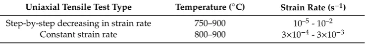
Table 1.Temperature and strain rate ranges of the uniaxial tensile test.
Uniaxial Tensile Test Type Temperature (◦C) Strain Rate (s−1)
Step-by-step decreasing in strain rate 750–900 10–5- 10–2 Constant strain rate 800–900 3×10⁻⁴- 3×10⁻³
3. Results
3.1. Microstructure Analysis after Annealing
Figure1shows the microstructures after annealing for 30 min in a temperature range of 750–900
◦
Materials2019,12, 1756 4 of 20
lower experimentalβ-fraction compared to the equilibriumβ-fraction was as a result of the lower diffusivity at temperatures below 825◦C and the insufficient annealing time required to finish the
α→βtransformation. Thus,α→βtransformation needed more than 30 min to provide an equilibrium state of the alloy in a temperature range of 750 to 800◦C.
Materials 2019, 12, x FOR PEER REVIEW 4 of 20
Table 1. Temperature and strain rate ranges of the uniaxial tensile test.
Uniaxial tensile test type Temperature (°C) Strain rate (s-1)
Step-by-step decreasing in strain rate 750–900 10–5 - 10–2
Constant strain rate 800–900 3×10⁻⁴ - 3×10⁻³
3. Results
3.1. Microstructure analysis after annealing
Figure 1 shows the microstructures after annealing for 30 min in a temperature range of 750–900
°C with a step of 25 °C. The β-phase volume fraction increased from 17% at 750 °C to 60% at 900 °C
(Figure 1). The temperature of α ≈ β (T50/50) was between 875–900 °C (Figure 1h). The measured
(solid lines in Figure 1h) and theoretical equilibrium (dotted lines in Figure 1h) values of phase ratio
were in good agreement within the temperature range of 825–900 °C (Figure 1h). The obtained lower
experimental β-fraction compared to the equilibrium β-fraction was as a result of the lower diffusivity
at temperatures below 825 °C and the insufficient annealing time required to finish the α→β
transformation. Thus, α→β transformation needed more than 30 min to provide an equilibrium state
of the alloy in a temperature range of 750 to 800 °C.
Fine β-grains were observed at 750 °C (Figure 1a) and the subsequent grain growth was due to
increased annealing temperature (Figure 1f). The mean β-grain size increased from 1.5 ± 0.2 to 2.1 ±
0.2 µ m in a temperature range of 750–825 °C. A temperature induced grain growth in the β-phase
was significant at temperatures above 825 °C. The mean grain size increased in two folds from 2.0 ±
0.2 µ m to 4.2 ± 0.2 µ m with increasing annealing temperature from 825–900 °C (Figure 1h). The α
-grains slightly grew from 3.2 ± 0.2 to 3.9 ± 0.3 µ m with increasing annealing temperature from 750 to
900 °C. Relatively coarse β-grains (4.2 ± 0.2 µ m) were also observed at 900 °C, after the annealing
process (Figure 1g).
Figure 1. Microstructure evolution of the investigated alloy after 30 min annealing at different temperatures: (a) 750 °C, (b) 800 °C, (c) 825 °C, (d) 850 °C, (e) 875OC and (f) 900 °C; (g) quantitative analysis of grain size, (h) quantitative analysis of volume fraction.
[image:4.595.89.502.155.428.2]3.2. Superplastic characteristics
Figure 1. Microstructure evolution of the investigated alloy after 30 min annealing at different temperatures: (a) 750◦C, (b) 800◦C, (c) 825◦C, (d) 850◦C, (e) 875OC and (f) 900◦C; (g) quantitative analysis of grain size, (h) quantitative analysis of volume fraction.
Fineβ-grains were observed at 750◦C (Figure1a) and the subsequent grain growth was due to increased annealing temperature (Figure1f). The meanβ-grain size increased from 1.5±0.2 to
2.1±0.2µm in a temperature range of 750–825◦
C. A temperature induced grain growth in theβ-phase was significant at temperatures above 825 ◦C. The mean grain size increased in two folds from 2.0±0.2µm to 4.2±0.2µm with increasing annealing temperature from 825–900◦C (Figure1h). The
α-grains slightly grew from 3.2±0.2 to 3.9±0.3µm with increasing annealing temperature from 750
to 900◦
C. Relatively coarseβ-grains (4.2±0.2µm) were also observed at 900◦
C, after the annealing process (Figure1g).
3.2. Superplastic Characteristics
3.2.1. Step-by-Step Reduction of Strain Rate Test
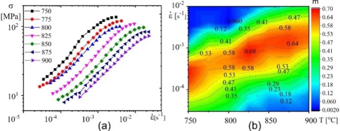
The superplastic characteristics were determined using a step-by-step reduction of strain rate test to evaluate the strain rate range of superplasticity in a temperature range of 750–900◦C. The strain rate sensitivity index (m) is a major indicator of superplasticity. The m is calculated by taking the slope of the Log stress-Log strain rate lines (m=∆(Log(σ))/∆(Log(´ε))). The material is considered to be under superplastic conditions when m≥0.3. Figure2a shows the logarithmic plots of flow stress vs.
Materials2019,12, 1756 5 of 20
1×10⁻³s−1in a temperature range of 825–900◦C (Figure2b). Even though the lower temperatures
(700–800◦C) also led to high m-values, they produced a lower strain rate at high flow stress values which are undesirable for SPF processes.
Materials 2019, 12, x FOR PEER REVIEW 5 of 20
3.2.1. Step-by-step reduction of strain rate test
The superplastic characteristics were determined using a step-by-step reduction of strain rate
test to evaluate the strain rate range of superplasticity in a temperature range of 750–900°C. The strain
rate sensitivity index (m) is a major indicator of superplasticity. The m is calculated by taking the
slope of the Log stress-Log strain rate lines (m = Δ(Log(σ))/ Δ(Log(έ))). The material is considered to
be under superplastic conditions when m ≥ 0.3. Figure 2a shows the logarithmic plots of flow stress
vs. strain rate curves. The curves exhibited sigmoidal shapes which are typical of superplastic behaviour. With an increase in deformation temperature, the linear part of the curve which corresponds to the maximum strain rate sensitivity (m) and superplastic behaviour, shifted towards high strain rates values and the flow stress values also decreased. The m-value exceeded 0.5 at strain
rates above 1 × 10⁻³ s−1 in a temperature range of 825–900 °C (Figure 2b). Even though the lower
temperatures (700–800 °C) also led to high m-values, they produced a lower strain rate at high flow
[image:5.595.121.470.143.278.2]stress values which are undesirable for SPF processes.
Figure 2. (a) Log stress-Log strain rate curves at a temperature range of 700 °C–900 °C obtained by a tensile test with step-by-step increment techniques. (b) The strain rate sensitivity index m.
3.2.2 . Constant strain rate tests
Figure 3 illustrates the true stress-strain curves (a–d), elongation-to-failure (e) and strain
hardening coefficient (n) (f) in the studied temperature-strain rate range.
Figure 3. Stress dependence on strain at various temperatures and various strain rates: (a) 4 × 10⁻⁴ s−1, (b) 6 × 10⁻⁴ s−1, (c)1 × 10⁻³ s−1, (d) 3 × 10⁻³ s−1, (e) elongation-to-failure, and (f) strain hardening coefficient (n).
Figure 2.(a) Log stress-Log strain rate curves at a temperature range of 700◦C–900◦C obtained by a tensile test with step-by-step increment techniques. (b) The strain rate sensitivity index m.
3.2.2. Constant Strain Rate Tests
Figure3illustrates the true stress-strain curves (a–d), elongation-to-failure (e) and strain hardening coefficient (n) (f) in the studied temperature-strain rate range.
Materials 2019, 12, x FOR PEER REVIEW 5 of 20
3.2.1. Step-by-step reduction of strain rate test
The superplastic characteristics were determined using a step-by-step reduction of strain rate
test to evaluate the strain rate range of superplasticity in a temperature range of 750–900°C. The strain
rate sensitivity index (m) is a major indicator of superplasticity. The m is calculated by taking the
slope of the Log stress-Log strain rate lines (m = Δ(Log(σ))/ Δ(Log(έ))). The material is considered to
be under superplastic conditions when m ≥ 0.3. Figure 2a shows the logarithmic plots of flow stress
vs. strain rate curves. The curves exhibited sigmoidal shapes which are typical of superplastic behaviour. With an increase in deformation temperature, the linear part of the curve which corresponds to the maximum strain rate sensitivity (m) and superplastic behaviour, shifted towards high strain rates values and the flow stress values also decreased. The m-value exceeded 0.5 at strain
rates above 1 × 10⁻³ s−1 in a temperature range of 825–900 °C (Figure 2b). Even though the lower
temperatures (700–800 °C) also led to high m-values, they produced a lower strain rate at high flow
stress values which are undesirable for SPF processes.
Figure 2. (a) Log stress-Log strain rate curves at a temperature range of 700 °C–900 °C obtained by a tensile test with step-by-step increment techniques. (b) The strain rate sensitivity index m.
3.2.2 . Constant strain rate tests
Figure 3 illustrates the true stress-strain curves (a–d), elongation-to-failure (e) and strain
hardening coefficient (n) (f) in the studied temperature-strain rate range.
[image:5.595.95.499.380.589.2]Figure 3. Stress dependence on strain at various temperatures and various strain rates: (a) 4 × 10⁻⁴ s−1, (b) 6 × 10⁻⁴ s−1, (c)1 × 10⁻³ s−1, (d) 3 × 10⁻³ s−1, (e) elongation-to-failure, and (f) strain hardening coefficient (n).
Figure 3.Stress dependence on strain at various temperatures and various strain rates: (a) 4×10⁻⁴s−1, (b) 6×10⁻⁴s−1, (c) 1×10⁻³s−1, (d) 3×10⁻³s−1, (e) elongation-to-failure, and (f) strain hardening coefficient (n).
The steady stage was characterized by strain hardening or softening which were observed to commence at a strain of nearly 0.1 (Figure3a–d). The strain hardening coefficient decreased with increasing strain rate and decreasing temperature (Figure3f). A strain rate of 3 × 10⁻³ s−1 in a
temperature range of 800–850◦C led to strain softening while strain hardening was observed at 900◦C with lower strain rates (3–6×10⁻⁴ s−1) (Figure 3a–c). In the studied strain rate range of
(0.3–3)×10−3
s−1, the elongation-to-failure exceeded 400% in a temperature range of 800–900◦C. It should be noted that, the maximum mean elongation-to-failure of 635% was obtained at a temperature of 825◦C and strain rate of 1 ×10⁻³ s−1(Figure 3e). This temperature is comparatively low for
Materials2019,12, 1756 6 of 20
At strain rate of 1×10⁻³s−1, a limited strain softening withn=0.06 was observed at 825◦C,
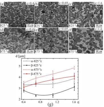
while strain hardening withn=0.25 was observed at 875◦C (Figure3f). To analyse the strain-induced grain structure changes, the samples after superplastic deformation at 825 and 875◦C with a strain rate of 1×10⁻³s−1and strains of 0.4, 0.69 and 1.6 were studied (Figure4). Theα-grains exhibit a stable size of 3.3±0.3µm and theβ-grains slightly decreased from 2.7±0.3 to 2.4±0.2µm with increasing
strain from 0.4 to 1.1 at 825◦C (Figure4a–c,e). The increasing strains resulted in an insignificant grain growth in both phases at higher values. In sharp contrast, monotonic grain growth was observed in both phases at 875◦C (Figure4d–g).
Materials 2019, 12, x FOR PEER REVIEW 6 of 20
The steady stage was characterized by strain hardening or softening which were observed to commence at a strain of nearly 0.1 (Figure 3a-d). The strain hardening coefficient decreased with
increasing strain rate and decreasing temperature (Figure 3f). A strain rate of 3 × 10⁻³ s-1 in a
temperature range of 800–850 °C led to strain softening while strain hardening was observed at
900 °C with lower strain rates (3–6 × 10⁻⁴ s-1) (Figure 3a–c). In the studied strain rate range of (0.3–3) ×
10-3 s-1, the elongation-to-failure exceeded 400% in a temperature range of 800–900 °C. It should be
noted that, the maximum mean elongation-to-failure of 635% was obtained at a temperature of 825 °C
and strain rate of 1 × 10⁻³ s-1 (Figure 3e). This temperature is comparatively low for conventional
Ti-6Al-4V alloy.
At strain rate of 1 × 10⁻³ s-1, a limited strain softening with n = 0.06 was observed at 825 °C, while
strain hardening with n = 0.25 was observed at 875 °C (Figure 3f). To analyse the strain-induced grain
structure changes, the samples after superplastic deformation at 825 and 875 °C with a strain rate of
1 × 10⁻³ s-1 and strains of 0.4, 0.69 and 1.6 were studied (Figure 4). The α-grains exhibit a stable size of
3.3 ± 0.3 μm and the β-grains slightly decreased from 2.7 ± 0.3 to 2.4 ± 0.2 µ m with increasing strain
from 0.4 to 1.1 at 825 °C (Figure4 a-c,e). The increasing strains resulted in an insignificant grain growth in both phases at higher values. In sharp contrast, monotonic grain growth was observed in
[image:6.595.116.481.205.580.2]both phases at 875°C (Figure 4 d–g).
Figure 4. Microstructure evolution after 0.4, 0.69, and 1.6 strain at a temperature of (a–c) 825°C, (d–f) 875 °C and (g) grain sizes-strain dependence.
Figures 5 and 6 present the EBSD grain-subgrain boundaries maps, grain diameter and
misorientation angle distributions for the samples deformed at 1 × 10⁻³ s-1 with strains of 0.4, 0.69, and
1.6. The analysis was done for the test samples with deformation temperatures of 825 and 875 °C. It
is known that, the β-phase partially transforms from BCC lattice to HCP lattice when the sample is
Figure 4. Microstructure evolution after 0.4, 0.69, and 1.6 strain at a temperature of (a–c) 825◦C, (d–f) 875◦C and (
g) grain sizes-strain dependence.
Figures 5 and 6 present the EBSD grain-subgrain boundaries maps, grain diameter and misorientation angle distributions for the samples deformed at 1 × 10⁻³ s−1 with strains of 0.4,
Materials2019,12, 1756 7 of 20
Materials 2019, 12, x FOR PEER REVIEW 7 of 20
cooled from high temperature to room temperature. Therefore, the measured grain diameter values
were matched to the HCP lattice structure (transformed β-phase and α-phase).
At 825 °C, the grain size was generally stable, with mean value of 3.2–3.3 μm (Figure 5 a–c). In
the as-deformed samples, the α-grains are normally distributed with a standard deviation of 1.8, 1.7,
and 1.6 for 0.4, 0.69, and 1.6 strains, respectively. This is reflective of the fact that the grain structure
was uniform (Figure 5d–f). During the deformation, the volume fraction of low-angle grain
boundaries (< 15°, LAGBs) decreased moderately, while that of high-angle grain boundaries (≥ 15°,
HAGBs) increased (Figure 5g–i). The fraction of the LAGBs < 15° at 0.4, 0.69, and 1.6 strains were
25.75%, 19.10%, and 14.50%, respectively. After 1.6 strain, the fraction of the LAGBs < 15° decreased by 0.65 times relative to those observed after 0.4 strain. This observation indicates the stability of attained grains during the deformation process.
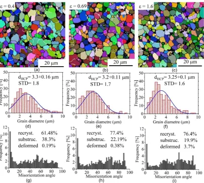
Figure 5. Electron backscattered diffraction (EBSD) grain-subgrain boundaries maps (a–c), grain size distribution (d–f) and the misorientation angle (g–i) at 1 × 10⁻³ s-1 and 825 °C for the HCP phase.
At 875 °C, the grains were dynamically grown with an increase in strain (Figure 6a–c). The grain
sizes and their distribution at 1 × 10⁻³ s-1 and 875 °C are presented in Figure 6d-f. The α-grains were
still normally distributed but with higher standard deviation than those at 825 °C for the same strains. Thus, the grain structure was less uniform at 875 °C. Similarly, at 825 °C, the volume fraction of
low-angle grain boundaries (< 15°, LAGBs) decreased, while that of high-angle grain boundaries (≥ 15°,
HAGBs) increased with the increasing strain (Figure 6g–i). The fraction of the LAGBs at 0.4 strain
[image:7.595.96.503.87.452.2]was smaller than those at 825 °C which reveals a high level of recrystallization under high temperature.
Figure 5.Electron backscattered diffraction (EBSD) grain-subgrain boundaries maps (a–c), grain size distribution (d–f) and the misorientation angle (g–i) at 1×10⁻³s−1and 825◦C for the HCP phase.
At 825◦C, the grain size was generally stable, with mean value of 3.2–3.3µm (Figure5a–c). In the as-deformed samples, theα-grains are normally distributed with a standard deviation of 1.8, 1.7, and 1.6 for 0.4, 0.69, and 1.6 strains, respectively. This is reflective of the fact that the grain structure was uniform (Figure5d–f). During the deformation, the volume fraction of low-angle grain boundaries (< 15◦, LAGBs) decreased moderately, while that of high-angle grain boundaries (≥15◦, HAGBs) increased
(Figure5g–i). The fraction of the LAGBs<15◦at 0.4, 0.69, and 1.6 strains were 25.75%, 19.10%, and 14.50%, respectively. After 1.6 strain, the fraction of the LAGBs<15◦decreased by 0.65 times relative to those observed after 0.4 strain. This observation indicates the stability of attained grains during the deformation process.
At 875◦C, the grains were dynamically grown with an increase in strain (Figure6a–c). The grain sizes and their distribution at 1×10⁻³s−1
and 875◦C are presented in Figure6d–f. Theα-grains were still normally distributed but with higher standard deviation than those at 825◦C for the same strains. Thus, the grain structure was less uniform at 875◦C. Similarly, at 825◦C, the volume fraction of low-angle grain boundaries (<15◦, LAGBs) decreased, while that of high-angle grain boundaries (≥15◦,
Materials2019,12, 1756 8 of 20
[image:8.595.99.498.87.447.2]Materials 2019, 12, x FOR PEER REVIEW 8 of 20
Figure 6. Electron backscattered diffraction (EBSD) grain-subgrain boundaries maps (a–c), grain size distribution (d–f) and the misorientation angle (g–i) at 1 × 10⁻³ s-1 and 875 °C for the HCP phase.
The microstructures of the near-fracture zone of the samples tested at 825 and 875 °C with a
strain rate of 1 × 10⁻³ s-1 are shown in Figures 7b,c. Several small cavities were observed in the gauge
part before failure at 825 °C (Figure 7b). At 875 °C, the residual cavitation was more intense (Figure
7c). It is notable thatthe cavities at 825 °C were significantly finer than those observed at 875 °C. The
sizes of cavities were 1–5 and 3–10 µ m at 825 and 875 °C, respectively. Several small residual cavities
were also observed in the gauge part after strain of 525% for 825 °C at 1 × 10⁻³ s-1 (Figure 7a). The
[image:8.595.92.505.602.708.2]cavities were small, narrowly distributed and not large enough to cause fracture with 525% strain at 825 °C.
Figure 7. SEM microstructure of the investigated alloy at 1 × 10⁻³ s−1 and temperature of (a,b) 825 °C and (c) 875 °C.
3.3. Classical constitutive equations (CE)
Figure 6.Electron backscattered diffraction (EBSD) grain-subgrain boundaries maps (a–c), grain size distribution (d–f) and the misorientation angle (g–i) at 1×10⁻³s−1and 875◦C for the HCP phase.
The microstructures of the near-fracture zone of the samples tested at 825 and 875◦C with a strain rate of 1×10⁻³s−1are shown in Figure7b,c. Several small cavities were observed in the gauge part
before failure at 825◦C (Figure7b). At 875◦C, the residual cavitation was more intense (Figure7c). It is notable that the cavities at 825◦C were significantly finer than those observed at 875◦C. The sizes of cavities were 1–5 and 3–10µm at 825 and 875◦C, respectively. Several small residual cavities were also observed in the gauge part after strain of 525% for 825◦C at 1×10⁻³s−1(Figure7a). The cavities were
small, narrowly distributed and not large enough to cause fracture with 525% strain at 825◦C.
Materials 2019, 12, x FOR PEER REVIEW 8 of 20
Figure 6. Electron backscattered diffraction (EBSD) grain-subgrain boundaries maps (a–c), grain size distribution (d–f) and the misorientation angle (g–i) at 1 × 10⁻³ s-1 and 875 °C for the HCP phase.
The microstructures of the near-fracture zone of the samples tested at 825 and 875 °C with a
strain rate of 1 × 10⁻³ s-1 are shown in Figures 7b,c. Several small cavities were observed in the gauge
part before failure at 825 °C (Figure 7b). At 875 °C, the residual cavitation was more intense (Figure
7c). It is notable thatthe cavities at 825 °C were significantly finer than those observed at 875 °C. The
sizes of cavities were 1–5 and 3–10 µ m at 825 and 875 °C, respectively. Several small residual cavities
were also observed in the gauge part after strain of 525% for 825 °C at 1 × 10⁻³ s-1 (Figure 7a). The
cavities were small, narrowly distributed and not large enough to cause fracture with 525% strain at 825 °C.
Figure 7. SEM microstructure of the investigated alloy at 1 × 10⁻³ s−1 and temperature of (a,b) 825 °C and (c) 875 °C.
3.3. Classical constitutive equations (CE)
Materials2019,12, 1756 9 of 20
3.3. Classical Constitutive Equations (CE)
In this approach, a Zener–Hollomon parameter Z and an exponent equation (Equations (1) and (2)) were used to express the relation of temperature and strain rate(
.
ε)at elevated temperature (T) [33,38].
Z= ε..×exp(Q
RT) (1)
. ε=
A1×σn1×exp
−Q1
RT
−Power law(ασ <0.8) A2×exp(βσ)×exp
−Q2
RT
−Exponential law(ασ >1.2) A3×[sinh(ασ)]n2×exp
−Q3
RT
−Hyperbolic sine law f or allσ
(2)
where, A,β, n1, n2andαare the material constants, and Q (kJ/mol) is an effective activation energy, R
is 8.314 J/(mol·K).
3.3.1. Model Parameters Determination
The flow stress-strain curves which were obtained from tensile tests at constant strain rates (Figure3) were utilized to compute the equation constants. The computing procedure of the model Factors at a strain of 0.4 is presented below as a guide. By taking the natural logarithm of both sides of Equation 2, the following equations (Equations (3)–(5)) were obtained:
lnε. =lnA1+ n1lnσ− Q1
RT ⇒ n1= "∂
lnε.
∂lnσ #
T
(3)
lnε. =lnA2+βσ− Q2
RT ⇒ β= "∂
lnε.
∂σ
#
T
(4)
lnε. =lnA3+ n2ln sinh(ασ) − Q3
RT ⇒ n2= "
∂lnε.
∂ln[sin h(ασ)]
#
T
(5)
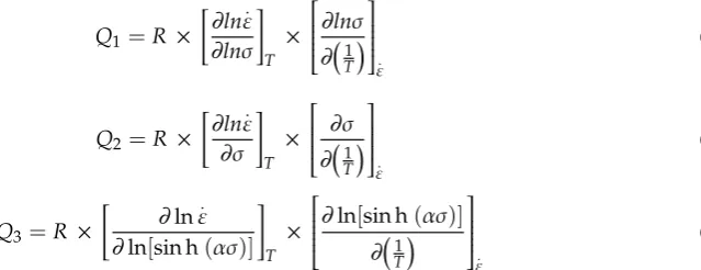
Q1,2,3(Equations (6)–(8)) was obtained by taking the partial differentiation of Equations (3)–(5).
Q1=R × "
∂lnε.
∂lnσ # T ×
∂lnσ
∂1 T . ε (6)
Q2=R × "
∂lnε.
∂σ # T × ∂σ ∂1 T . ε (7)
Q3=R × "
∂lnε.
∂ln[sin h(ασ)]
# T ×
∂ln[sin h(ασ)]
∂1 T . ε (8)
Figure8shows the linear plots of lnε. −lnσ(Figure8a), lnε.−σ(Figure8b), lnε. −ln sinh(ασ)
(Figure8c), and ln sin h(ασ)− 1000
RT (Figure8d). The average values of the inclined lines from ln
.
ε−lnσ
and lnε.−σcurves (Figure8a,b) are used to compute then1,β, andQ1,2. By the same way, the average
values of the inclined lines from lnε. −ln sinh(ασ)and ln sin h(ασ)− 1000
[image:9.595.188.508.481.604.2]Materials2019,12, 1756 10 of 20 Materials 2019, 12, x FOR PEER REVIEW 11 of 20
Figure 8. The plots of (a) ln 𝜀̇ − ln 𝜎; (b) ln 𝜀̇ − 𝜎; (c) plots of ln 𝜀̇ − ln sinh(𝛼𝜎); (d) ln sinh(𝛼𝜎) − 1000𝑅𝑇 .
3.3.2. The strain dependence of material constants
At a strain range of 0.1–1, the material constants n1,2, α, 𝑄1,3, and A1,3 were calculated to
determine the effect of strain on the constant values. The procedure to determine the solution of these constants was similar to those observed at a strain of 0.5. Figure 9 shows the dependence of material
constants vs.strain ε. The influence of strain on the material constants was regressed by a 3rd order
polynomial fitting method, which was the suitable order for the polynomial fitting Figure 9a. The material constants were significantly affected by the strains at all tested conditions. The fitting equations were expressed by Equation 16. The regressing coefficients of each equation are listed in Table 3.
The value of n1 andn2 had the samecharacteristics; they increased with the increasing strain
(Figure 9b). Thus, the (m) value decreased with increasing strain. The effective activation energy
𝑄1 𝑎𝑛𝑑 3 increased with increasing strain from 225 to 300 kJ/mol (Figure 9d). The 𝑄1 𝑎𝑛𝑑 3 vs. strain
dependence exhibited sigmoidal shape with a slight increase of 𝑄1 𝑎𝑛𝑑 3 in a strain range of 0.3–0.7
and a significant increase of the 𝑄1 𝑎𝑛𝑑 3 in a strain range of 0.7–1. Constant ln(A3) demonstrated a
similar behaviour (Figure 9d,e). However, ln(A1) exhibited an opposite characteristic, with trends
decreasing with an increase in strain (Figure 9e).
The relationship between the material constant α and the strain was dependent on the upward
parabola with values varying from 18.5–22 × 10-3. The strain of 0.7 provided the minimum value of α
constant (Figure 9c).
[image:10.595.94.503.428.468.2]Figure 8.The plots of (a) lnε.−lnσ; (b) lnε.−σ; (c) plots of lnε.−ln sinh(ασ); (d) ln sinh(ασ)−1000 RT .
Table 2.The computed values of the constants of both simple power law and hyperbolic sine equations.
ln(A1) n1/m * Q1
[KJ/mol] ln(A2)
β
[MPa−1]
Q2
[KJ/mol] α ln(A3) n2
Q3
[KJ/mol]
10.22 2.5/0.4 250.6 13.6 0.05 220.4 0.019 19 1.97 242
* The strain rate sensitivitym-index values were calculated asm=n1 1.
According to the power law function, the values of the strain rate and flow stress can be expressed as following (Equation (9)–(11)).
.
ε=A1σn1×exp
−Q1 RT
(9)
.
ε=2.77× 10⁴[σ2.58×exp
−250.6 × 1000 RT
] (10)
σ= z
A1 !n1
1
=
.
ε×exp250.6×1000
RT
2.77 × 10⁴ 1 2.58
(11)
Based on the hyperbolic sine function, which is used for various values of the strain rate, the flow stress can be expressed as following (Equations (12)–(15)).
.
ε=A3[sinh(ασ)]n2×exp(−Q3
RT) (12)
.
ε= 1.9 × 10⁸[sin h(0.019σ)]1.97×exp
−242 × 1000 RT
Materials2019,12, 1756 11 of 20
σ= 1
αln z A3
!n1 2 + z A3
!n2 2 +1 1 2 (14)
σ= 1
0.019ln .
ε×exp242×1000
RT
1.9 × 10⁸ 1 1.97 + .
ε×exp242×1000
RT
1.9 × 10⁸ 2 1.97 +1 1 2
(15)
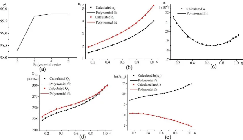
3.3.2. The Strain Dependence of Material Constants
At a strain range of 0.1–1, the material constants n1,2,α,Q1,3, and A1,3were calculated to determine
the effect of strain on the constant values. The procedure to determine the solution of these constants was similar to those observed at a strain of 0.5. Figure9shows the dependence of material constants vs. strainε. The influence of strain on the material constants was regressed by a 3rd order polynomial fitting method, which was the suitable order for the polynomial fitting Figure9a. The material constants were significantly affected by the strains at all tested conditions. The fitting equations were expressed by Equation 16. The regressing coefficients of each equation are listed in Table3.
Materials 2019, 12, x FOR PEER REVIEW 12 of 20
Figure 9. (a) Root mean square vs. the polynomial order, (b) variation of n1,2 vs. true strain (c) variation of α vs. true strain, (d) variation of 𝑄1,3, vs. true strain, and (e) variation of ln(A1,3) vs. true
strain (ε).
{
𝛼 = 𝑌0+ 𝐵1𝜀1+ 𝐵2𝜀2+ 𝐵3𝜀3
𝑛1,2 = 𝑌0+ 𝐵1𝜀1+ 𝐵2𝜀2+ 𝐵3𝜀3
𝐴1,3= 𝑌0+ 𝐵1𝜀1+ 𝐵2𝜀2+ 𝐵3𝜀3
𝑄1,3= 𝑌0+ 𝐵1𝜀1+ 𝐵2𝜀2+ 𝐵3𝜀3
(16)
Table 3. The coefficients of the polynomial fitting for α, n2, A3, and 𝑄3 and the R2 for this fitting.
Parameter Y0 B1 B2 B3
𝛼 0.024 -0.017 0.017 -0.004
𝑛1 1.516 3.243 -2.784 3.064
𝑛2 1.167 2.480 -2.153 2.355
ln(𝐴1) 10.607 3.451 -12.319 3.372
ln(𝐴3) 15.16 15.99 -21.95 15.06
𝑄1 212.00 159.94 -218.74 143.11
𝑄3 204.71 154.28 -217.34 154.6
Once the material constants at different strains were determined, the fitted flow stress can be
calculated using Equations 11–15 for both models. For evaluation of the performance and accuracy
of the models, the following comparative statistical terms were computed (Equations 17–20); where
Ei and Pi, are the experimental and the approximated flow stress values, 𝐸̅ and 𝑃,̅ are the mean
values of the experimental and approximated flow stress, and N is the total data number
correlation coefficient (𝑅) = ∑ (𝐸𝑖− 𝐸̅)
𝑁
𝑖=1 (𝑃𝑖− 𝑃̅)
√∑𝑁𝑖=1(𝐸𝑖− 𝐸̅)2∑𝑁𝑖=1(𝑃𝑖− 𝑃̅)2
(17)
average absolute relative error (𝐴𝐴𝑅𝐸) = 1 𝑁∑ |
𝐸𝑖− 𝑃𝑖
𝐸𝑖
|
𝑁
𝑖=1
[image:11.595.92.505.328.566.2](18)
Figure 9.(a) Root mean square vs. the polynomial order, (b) variation of n1,2 vs. true strain (c) variation ofαvs. true strain, (d) variation ofQ1,3, vs. true strain, and (e) variation of ln(A1,3) vs. true strain (ε).
Table 3.The coefficients of the polynomial fitting forα, n2, A3, andQ3and the R2for this fitting.
Parameter Y0 B1 B2 B3
α 0.024 −0.017 0.017 −0.004
n1 1.516 3.243 −2.784 3.064
n2 1.167 2.480 −2.153 2.355
ln(A1) 10.607 3.451 −12.319 3.372 ln(A3) 15.16 15.99 −21.95 15.06
Q1 212.00 159.94 −218.74 143.11
Q3 204.71 154.28 −217.34 154.6
Materials2019,12, 1756 12 of 20
Q1and3increased with increasing strain from 225 to 300 kJ/mol (Figure9d). TheQ1and3vs. strain
dependence exhibited sigmoidal shape with a slight increase ofQ1and3in a strain range of 0.3–0.7 and
a significant increase of theQ1and3in a strain range of 0.7–1. Constant ln(A3) demonstrated a similar
behaviour (Figure9d,e). However, ln(A1) exhibited an opposite characteristic, with trends decreasing with an increase in strain (Figure9e).
The relationship between the material constantαand the strain was dependent on the upward parabola with values varying from 18.5–22×10−3. The strain of 0.7 provided the minimum value ofα
constant (Figure9c).
α=Y0+B1ε1+B2ε2+B3ε3 n1,2=Y0+B1ε1+B2ε2+B3ε3 A1,3 =Y0+B1ε1+B2ε2+B3ε3 Q1,3=Y0+B1ε1+B2ε2+B3ε3
(16)
Once the material constants at different strains were determined, the fitted flow stress can be calculated using Equations (11)–(15) for both models. For evaluation of the performance and accuracy of the models, the following comparative statistical terms were computed (Equations (17)–(20)); where
EiandPi,are the experimental and the approximated flow stress values,EandP, are the mean values of the experimental and approximated flow stress, and N is the total data number.
correlation coefficient(R) =
PN
i=1
Ei− E
Pi− P
q
PN
i=1
Ei− E
2PN
i=1
Pi− P
2
(17)
average absolute relative error(AARE) = 1
N
N X
i=1
Ei− Pi
Ei
(18)
root mean square error(RMSE) =
v u t 1
N
N X
i=1
(Ei−Pi)2 (19)
Error= 1
εmax εmax Z
0
Ei.(ε)−Pi(ε)
dε (20)
Materials2019,12, 1756 13 of 20
Materials 2019, 12, x FOR PEER REVIEW 13 of 20
root mean square error (𝑅𝑀𝑆𝐸) = √1
𝑁∑(𝐸𝑖− 𝑃𝑖)2
𝑁
𝑖=1
(19)
𝐸𝑟𝑟𝑜𝑟 = 1 𝜀𝑚𝑎𝑥
∫ |𝐸𝑖.(𝜀) − 𝑃𝑖(𝜀)| 𝜀𝑚𝑎𝑥
0
𝑑𝜀 (20)
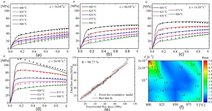
Figure 10 a–d and Figure 11a–d show the data of the experiment (lines) and the approximation
(scatters) made by both models’ flow stresses. Figure 10e–f and Figure 11e–f show the performance
and the error of the constructed model. Figure 10 shows that the flow stress can be best fitted and approximated by the power law constitutive model, because the approximated flow stresses are in
agreement with the tested stresses. The R, AARE, and RMSE values were 98.77%, 3.7%, and 2.16
(Figure 10e) respectively. The overall error (Error) is shown in (Figure 10f).
Figure 10. Comparative plots for the experimental results (lines) and fitted values by power law model (symbols) at (a) 4 × 10⁻⁴ s−1, (b) 6 × 10⁻⁴ s−1, (c)1 × 10⁻³ s−1, and (d) 3× 10⁻³ s−1; (e) the correlation between experimental and fitted flow stress; (f) the error between experimental and tested flow stress.
The hyperbolic sine law model also revealed a good fitting of the model and experimental
values. The R, AARE, and RMSE values were 98.84%, 4.4%, and 2.05 (Figure 11e), respectively. The
[image:13.595.93.501.87.300.2]overall error (Error) is shown in (Figure 11f).
Figure 10.Comparative plots for the experimental results (lines) and fitted values by power law model (symbols) at (a) 4×10⁻⁴s−1, (b) 6×10⁻⁴s−1, (c) 1×10⁻³s−1, and (d) 3×10⁻³s−1; (e) the correlation between experimental and fitted flow stress; (f) the error between experimental and tested flow stress.
Materials 2019, 12, x FOR PEER REVIEW 14 of 20
Figure 11. Comparative plots for the experimental results (lines) and fitted values by hyperbolic sine law model (symbols) at (a) 4 × 10⁻⁴ s−1, (b) 6 × 10⁻⁴ s−1, (c) 1 × 10⁻³ s−1 , and (d) 3× 10⁻³ s−1 ; (e) the correlation between experimental and fitted flow stress; (f) the error between experimental and tested flow stress.
3.3.3. Cross-approval of the suggested models
In this approach, a cross-validation procedure was employed in order to determine which constructed model; power law or hyperbolic sine law, can accurately predict the deformation behaviour of the studied alloy. The constructed models were proved by separating the tested flow stress-strain plots from each other. A twenty-trial dataset with various deformation temperatures and strain rates were performed (Table 4). The constructed models were rebuilt afterwards for each trial dataset and the predictions done for conditions of excluded stress-strain plot. In addition, the predicted values were compared with the tested data.
Table 4. The excluded conditions in trial datasets.
Trial Number Excluded conditions Trial Number Excluded conditions T (°C) 𝜀̇ (s−1) T (°C) 𝜀̇ (s−1)
Trial 1 800 3 x 10⁻⁴ Trial 11 850 1 x 10⁻³
Trial 2 800 6 × 10⁻⁴ Trial 12 850 3 x 10⁻³
Trial 3 800 1 x 10⁻³ Trial 13 875 3 x 10⁻⁴
Trial 4 800 3 x 10⁻³ Trial 14 875 6 x 10⁻⁴
Trial 5 825 3 x 10⁻⁴ Trial 15 875 1 x 10⁻³
Trial 6 825 6 x 10⁻⁴ Trial 16 875 3 x 10⁻³
Trial 7 825 1 x 10⁻³ Trial 17 900 3 x 10⁻⁴
Trial 8 825 3 x 10⁻³ Trial 18 900 6 x 10⁻⁴
Trial 9 850 3 x 10⁻⁴ Trial 19 900 1 x 10⁻³
Trial 10 850 6 x 10⁻⁴ Trial 20 900 3 x 10⁻³
Figure 12 demonstrates the dependence of n1, n2, Q1, and Q3 versus strain for all trials. The
material property factors nearly show similar characteristics with an increase in strain for all trials
[image:13.595.98.500.360.569.2](Figure 12a–d).
Figure 11.Comparative plots for the experimental results (lines) and fitted values by hyperbolic sine law model (symbols) at (a) 4×10⁻⁴s−1, (b) 6×10⁻⁴s−1, (c) 1×10⁻³s−1, and (d) 3×10⁻³s−1; (e) the correlation between experimental and fitted flow stress; (f) the error between experimental and tested flow stress.
The hyperbolic sine law model also revealed a good fitting of the model and experimental values. TheR, AARE, and RMSE values were 98.84%, 4.4%, and 2.05 (Figure11e), respectively. The overall error (Error) is shown in (Figure11f).
3.3.3. Cross-Approval of the Suggested Models
Materials2019,12, 1756 14 of 20
[image:14.595.113.483.157.311.2]were performed (Table4). The constructed models were rebuilt afterwards for each trial dataset and the predictions done for conditions of excluded stress-strain plot. In addition, the predicted values were compared with the tested data.
Table 4.The excluded conditions in trial datasets.
Trial Number
Excluded Conditions
Trial Number
Excluded Conditions
T (◦C) ˙
ε(s−1) T (◦C) ˙ ε(s−1)
Trial 1 800 3×10⁻⁴ Trial 11 850 1×10⁻³
Trial 2 800 6×10⁻⁴ Trial 12 850 3×10⁻³
Trial 3 800 1×10⁻³ Trial 13 875 3×10⁻⁴
Trial 4 800 3×10⁻³ Trial 14 875 6×10⁻⁴
Trial 5 825 3×10⁻⁴ Trial 15 875 1×10⁻³
Trial 6 825 6×10⁻⁴ Trial 16 875 3×10⁻³
Trial 7 825 1×10⁻³ Trial 17 900 3×10⁻⁴
Trial 8 825 3×10⁻³ Trial 18 900 6×10⁻⁴
Trial 9 850 3×10⁻⁴ Trial 19 900 1×10⁻³
Trial 10 850 6×10⁻⁴ Trial 20 900 3×10⁻³
Figure12demonstrates the dependence ofn1,n2, Q1,and Q3versus strain for all trials. The
material property factors nearly show similar characteristics with an increase in strain for all trials (Figure12a–d).
Materials 2019, 12, x FOR PEER REVIEW 15 of 20
Figure 12. Variation of n1, n2, Q1, and Q3 with true strain for all trails: (a) n1, (b) n2, (c) Q1, and (d)
Q3.
Figure 13. The error between experimental and tested flow stress after cross-validation of (a) power law model and (b) hyperbolic sine law model.
The cross-validation technique revealed that both models exhibited a low level of errors. Thus, both models can be used to correctly predict the flow behaviour of this alloy (Figure 13). The power law model exhibited only one critical region (lowest temperature-highest strain rate) with an error of 7% (Figure 13a). In the case of hyperbolic sine law, the extreme points (lowest tested temperature-highest strain rate and temperature-highest temperature-lowest strain rate) exhibited higher error compared with the other points (Figure 13b). Therefore, the proposed power law model had better predictability of the stress values under superplastic deformation.
4. Discussion
The material constants in the CE model indicate the deformation-controlling mechanisms in the studied temperature-strain rate range. The mechanisms can be evaluated by using the stress exponent
values n1,2 andan effective activation energy (𝑄1,3) [39].Grain boundary sliding (GBS) mechanism is
[image:14.595.102.494.383.647.2]considered to be dominant at n1,2 values close to 2. For dislocation viscous glide (DVG), it is assumed
Figure 12.Variation of n1, n2, Q1, and Q3 with true strain for all trails: (a) n1, (b) n2, (c) Q1, and (d) Q3.
Materials2019,12, 1756 15 of 20 Materials 2019, 12, x FOR PEER REVIEW 15 of 20
Figure 12. Variation of n1, n2, Q1, and Q3 with true strain for all trails: (a) n1, (b) n2, (c) Q1, and (d)
Q3.
Figure 13. The error between experimental and tested flow stress after cross-validation of (a) power law model and (b) hyperbolic sine law model.
The cross-validation technique revealed that both models exhibited a low level of errors. Thus, both models can be used to correctly predict the flow behaviour of this alloy (Figure 13). The power law model exhibited only one critical region (lowest temperature-highest strain rate) with an error of 7% (Figure 13a). In the case of hyperbolic sine law, the extreme points (lowest tested temperature-highest strain rate and temperature-highest temperature-lowest strain rate) exhibited higher error compared with the other points (Figure 13b). Therefore, the proposed power law model had better predictability of the stress values under superplastic deformation.
4. Discussion
The material constants in the CE model indicate the deformation-controlling mechanisms in the studied temperature-strain rate range. The mechanisms can be evaluated by using the stress exponent
values n1,2 andan effective activation energy (𝑄1,3) [39].Grain boundary sliding (GBS) mechanism is
considered to be dominant at n1,2 values close to 2. For dislocation viscous glide (DVG), it is assumed
Figure 13.The error between experimental and tested flow stress after cross-validation of (a) power law model and (b) hyperbolic sine law model.
4. Discussion
The material constants in the CE model indicate the deformation-controlling mechanisms in the studied temperature-strain rate range. The mechanisms can be evaluated by using the stress exponent valuesn1,2and an effective activation energy (Q1,3) [39]. Grain boundary sliding (GBS) mechanism is
considered to be dominant atn1,2values close to 2. For dislocation viscous glide (DVG), it is assumed
atn2values close to 3 whereas that of dislocation climb (DC) mechanism is linked to n1,2 values from 4–6 [40,41]. For the studied alloy, the stress exponent valuesn2 was increased from 1.5 to 4 (Figure7a) which suggests that the controlling deformation mechanism was changed with increasing strain. At strains below 0.7, both GBS and DVG are supposed to be the deformation-controlling mechanisms according to the values ofn1,2. The nature of the deformation mechanisms can change with increasing strain. With increasing strain to 0.8, the value ofn1,2increased to 3 and dislocation viscous glide is considered as the main mechanism governing the deformation. At strains up to 1, the n2increased to 4, which projects dislocation climb as the deformation-controlling mechanism.
The Q-value increased from 225–300 kJ/mol with increasing strain to 1.1. These values are typically associated with the increasing role of thermally activated dislocation slip/creep mechanisms [32]. The increase in dislocation activity with decreasing temperature was in-situ observed in Ti-6Al-4V by Alabort [9].
The most important result in this study is the observation of higher elongation-to-failure at 825 compared to 875◦C. Considering both temperatures at a constant strain rate of 1×10⁻³s−1, the samples
[image:15.595.100.506.89.242.2]Materials2019,12, 1756 16 of 20
softening at 825◦C was as a result of dynamic recrystallization, slight grain refinement ofβ-phase and high stability ofα-grains. The superplastic deformation behaviour at 875◦C was controlled by a competition between dynamic recrystallization and dynamic grain growth. The strain hardening was as a result of the higher impact of dynamic grain growth on both phases rather than the grain refinement due to dynamic recrystallization.
Typically, at higher temperatures, cavity ‘initiation’ occurs at larger strains due to the increasing proportions of ductileβ-phase hence the increased diffusional accommodation of the GBS phenomenon according to Reference [51]. In our case, the finer grain structure was the main reason for lower cavitation and the finer cavities size at 825◦C provided 23±4% of ductileβ-phase as compared to
875◦
C which provided 40±6% ofβ-phase.
Superplastic deformation mechanisms are controlled by atomic diffusion. The diffusion rate in two-phased titanium alloys depends on the deformation temperature, grain size and the volume fraction of diffusiveβphase. The results of this study suggested that stable and finer grain size are more important to improving superplasticity of the studied alloy than increasing diffusivity. The increased diffusivity comes about by virtue of the increasing volume fraction of the high diffusive and ductileβ-phase due to increasing deformation temperature. Due to fine and stable grain structure, the lower temperature of 825◦C provided a necking free deformation, a higher elongation-to-failure, a lower cavitation, and an acceptable flow stress value. The same trend was observed by Guo et al. [49] for Ti-6Al-4V. The dynamic grain growth with increased cavitation resulted in a strain hardening and a lower elongation at 875◦C. This observation can change by relieving the grain boundary sliding and its accommodation with finer grains at 825◦C. The 20% of fine-grained ductile and diffusive
β-phase at 825◦C provided the effective accommodation for grain boundary sliding by diffusion and dislocation slip/creep mechanisms. It is important to note that only 20% ofβ-phase was optimum for a good superplasticity of the studied samples. A similarly low optimalβ-phase volume fraction was reported for Ti-6Al-2Sn-4Zr-2Mo-0.1Si [45] and Ti-6Al-4V alloy [10,13]. Softening accompanying the deformation process also suggests the presence of dynamic recrystallization and, as a result, increased the role of the dislocation mechanisms at 825◦C [8]. We suggest that the dynamic grain growth at 875◦C had a significant effect on the accommodation of grain boundary sliding, while the dislocation accommodation was more important at 825◦
C.
5. Conclusions
The microstructure and superplastic deformation behaviour of conventionally processed sheets of Ti-6Al-4V alloy were analysed in a temperature range of 750–900◦C and a strain rate range of 10–5–10–2s−1. The experimental stress-strain data of the constant strain rate tests were used to construct constitutive models for fitting and predicting the superplastic flow behaviour. Based on the results of this study we concluded that:
• For the studied alloy composition, the experimental and Thermo-Calc calculatedβ-phase fraction vs. temperature was in agreement, and theα/βfraction changed from≈80/20 at 750 to≈40/60 at
900◦C. Theα-grain size slightly increased from 3.2±0.20 to 3.9±0.25µm while theβ-grains grew significantly from 1.8±0.20 to 4.2±0.20µm with an increase in annealing temperature from
750 to 900◦C. For theβ-grains, a significant temperature-induced grain growth by 2 folds was observed in a temperature range of 850–900◦C.
• The alloy demonstrated superplasticity in a strain rate range of 6×10⁻⁴–3×10⁻³s−1and in
a temperature range of 800–900◦C. An elongation-to-failure>400% andm-value>0.45 were observed. The considerably low optimal deformation temperature of 825◦C, which provided the maximum superplastic elongation, was established. Due to the fine-structure and its stability during superplastic deformation, a maximum elongation–to-failure of 635% and stable flow with strain hardening coefficient close to zero were achieved at a constant strain rate of 1×10⁻³s−1
Materials2019,12, 1756 17 of 20
• The recrystallization process was not finished before the superplastic deformation process
commenced. Continuous dynamic recrystallization accompanied by decreasing volume fraction of low angle grain boundaries occurred at superplastic deformation, as shown by the EBSD study.
• A comparison of the experimental and approximated flow stresses indicated that, the constitutive
models based on both power law and hyperbolic sine equations exhibited high accuracy and good efficiency in fitting and approximating the superplastic deformation behaviour of the studied alloy. The predictability of both developed models was compared using the cross-validation approach. The constitutive model based on the power law equation exhibited excellent predictability of the stress-strain superplastic behaviour of the alloy.
Author Contributions:Conceptualization, A.O.M. and A.D.K.; methodology, A.D.K.; software, A.V.M.; validation, A.O.M., A.D.K. and J.S.K.; formal analysis, A.V.M.; investigation, A.D.K.; resources, S.A.A; data curation, A.O.D.; writing—original draft preparation, A.V.M.; writing—review and editing, J.S.K; visualization, A.D.K.; supervision, A.V.M.
Funding:This research was funded by RSF, grant number Grant #18-79-00348.
Acknowledgments: The authors wish to dedicate this work to the memory of V.K. Portnoy. We are extremely thankful for his guidance, patience and support. He was always nice, calm, and he taught us how to be always optimistic, even in the dark.
Conflicts of Interest: The authors declare no conflict of interest. The funders had no role in the design of the study; in the collection, analyses, or interpretation of data; in the writing of the manuscript, or in the decision to publish the results.
Nomenclature
Symbol/Acronym Full name Symbol/Acronym Full name
SPF Superplastic forming ε True strain
CE Constitutive equations ε. Deformation strain rate (s-1)
R correlation coefficient T Deformation temperature
(◦C)
AARE mean absolute relative error m Strain rate sensitivity index
RMSE root mean square error GBS Grain boundary sliding
ANN artificial neural network A,β, n1, n2 andα Material constants
α Titanium alpha-phase (HCP) Q Effective activation energy (kJ/mol)
β Titanium beta phase (BCC) R gas constant 8.314 J/(mol·K).
SEM Scanning electron
microscope α
0
Returned beta phase
LAGB low-angle grain boundary EBSD Electron backscatter diffraction
σ Flow stress (MPa) HAGB high-angle grain boundary
References
1. Langdon, T.G. The physics of superplastic deformation.Mater. Sci. Eng. A1991,137, 1–11. [CrossRef] 2. Kawasaki, M.; Langdon, T.G. Superplasticity in ultrafine-grained materials.Rev. Adv. Mater. Sci.2018,54,
46–55. [CrossRef]
3. Leyens, C.; Peters, M.Titanium an Titanium Alloys, Wiley-VCH: Weinheim, Germany, 2002; ISBN 3527305343. 4. Sieniawski, J.; Motyka, M. Superplasticity in titanium alloys.J. Achiev. Mater. Manuf. Eng.2007,24, 123–130. 5. Nieh, T.G.; Wadsworth, J.; Sherby, O.D.Superplasticity in metals and ceramics; Cambridge University Press:
New York, NY, USA, 2014; ISBN 9780874216561.
Materials2019,12, 1756 18 of 20
7. Kaibyshev, O.A.Superplasticity of Alloys, Intermetallides and Ceramics, Springer-Verlag: Berlin/Heidelberg, Germany, 1992; ISBN 978-3-642-84675-5.
8. Alabort, E.; Putman, D.; Reed, R.C. Superplasticity in Ti-6A-4V: Characterisation, modelling and applications.
Acta Mater.2015,95, 428–442. [CrossRef]
9. Alabort, E.; Kontis, P.; Barba, D.; Dragnevski, K.; Reed, R.C. On the mechanisms of superplasticity in Ti-6Al-4V.Acta Mater.2016,105, 449–463. [CrossRef]
10. Seshacharyulu, T.; Medeiros, S.C.; Frazier, W.G.; Prasad, Y.V.R.K. Hot working of commercial Ti–6Al–4V with an equiaxedα–βmicrostructure: materials modeling considerations.Mater. Sci. Eng. A2000,284, 184–194. [CrossRef]
11. Matsumoto, H.; Nishihara, T.; Velay, V.; Vidal, V. Superplastic Property of the Ti–6Al–4V Alloy with Ultrafine-Grained Heterogeneous Microstructure.Adv. Eng. Mater.2018,20, 1–6. [CrossRef]
12. Xiao, J.; Li, D.S.; Li, X.Q.; Deng, T.S. Constitutive modeling and microstructure change of Ti-6Al-4V during the hot tensile deformation.J. Alloys Compd.2012,541, 346–352. [CrossRef]
13. Ko, Y.G.; Lee, C.S.; Shin, D.H.; Semiatin, S.L. Low-Temperature Superplasticity of Ultra-Fine-Grained Ti-6Al-4V Processed by Equal-Channel Angular Pressing. Metall. Mater. Trans. A2006, 37, 381–391. [CrossRef]
14. Gao, F.; Li, W.; Meng, B.; Wan, M.; Zhang, X.; Han, X. Rheological law and constitutive model for superplastic deformation of Ti-6Al-4V.J. Alloys Compd.2017,701, 177–185. [CrossRef]
15. Mosleh, A.O.; Mikhaylovskaya, A.; Kotov, A.D.; AbuShanab, W.; Moustafa, E.; Portnoy, V. Experimental Investigation of the Effect of Temperature and Strain Rate on the Superplastic Deformation Behavior of Ti-Based Alloys in the (α+β) Temperature Field.Metals2018,8, 819. [CrossRef]
16. Vanderhasten, M.; Rabet, L.; Verlinden, B. Deformation mechanisms of Ti-6Al-4V during tensile behavior at low strain rate.J. Mater. Eng. Perform.2007,16, 208–212. [CrossRef]
17. Zhang, X.; Zhang, S.; Zhao, Q.; Zhao, Y.; Li, R.; Zeng, W. In-situ observations of the tensile deformation and fracture behavior of a fine-grained titanium alloy sheet.J. Alloys Compd.2018,740, 660–668. [CrossRef] 18. Liu, Q.; Hui, S.; Tong, K.; Yu, Y.; Ye, W.; Song, S. yin Investigation of high temperature behavior and
processing map of Ti-6Al-4V-0.11Ru titanium alloy.J. Alloys Compd.2019,787, 527–536. [CrossRef] 19. Jha, J.S.; Toppo, S.P.; Singh, R.; Tewari, A.; Mishra, S.K. Flow stress constitutive relationship between lamellar
and equiaxed microstructure during hot deformation of Ti-6Al-4V.J. Mater. Process. Technol. 2019,270, 216–227. [CrossRef]
20. Tchein, G.J.; Jacquin, D.; Aldanondo, E.; Coupard, D.; Gutierrez-Orrantia, E.; Girot Mata, F.; Lacoste, E. Analytical modeling of hot behavior of Ti-6Al-4V alloy at large strain. Mater. Des. 2019,161, 114–123. [CrossRef]
21. Wang, J.; Xu, Y.; Zhang, W.; Wang, W. A finite-strain thermomechanical model for severe superplastic deformation of Ti-6Al-4V at elevated temperature.J. Alloys Compd.2019,787, 1336–1344. [CrossRef] 22. Zhou, G.; Chen, L.; Liu, L.; Liu, H.; Peng, H.; Zhong, Y. Low-Temperature Superplasticity and Deformation
Mechanism of Ti-6Al-4V Alloy.Materials (Basel)2018,11, 1212. [CrossRef]
23. Akihiko, C. Superplasticity of the Ultrafine-Grained Ti-6A Al-4V Alloy with a Metas stable -Single Phase Microstructure.Proc. 13th World Conf. Titan.2016, 789–792. [CrossRef]
24. Zherebtsov, S.V.; Kudryavtsev, E.A.; Salishchev, G.A.; Straumal, B.B.; Semiatin, S.L. Microstructure evolution and mechanical behavior of ultrafine Ti6Al4V during low-temperature superplastic deformation.Acta Mater. 2016,121, 152–163. [CrossRef]
25. Yang, P.R.; Cai, M.H.; Wu, C.F.; Su, J.H.; Guo, X.P. Strain-rate dependent hot deformation behavior and mechanism of interphase- precipitated Ti-Mo-xNb steels: Physical modeling and characterization.Mater. Sci. Eng. A2018,729, 230–240. [CrossRef]
26. Wang, X.D.; Pan, Q.L.; Xiong, S.W.; Liu, L.L.; Sun, Y.W.; Wang, W.Y. Prediction on hot deformation behavior of spray-formed 7055 aluminum alloy via phenomenological models.Trans. Nonferrous Met. Soc. China2018,
28, 1484–1494. [CrossRef]