This is a repository copy of
Local Binary Patterns for Graph Characterization
.
White Rose Research Online URL for this paper:
http://eprints.whiterose.ac.uk/132052/
Version: Accepted Version
Conference or Workshop Item:
Jawad, Mohammed, Aziz, Furqan and Hancock, Edwin R orcid.org/0000-0003-4496-2028
(Accepted: 2018) Local Binary Patterns for Graph Characterization. In: 24th International
Conference on Pattern Recognition, 21-24 Aug 2018. (In Press)
[email protected] https://eprints.whiterose.ac.uk/
Reuse
Items deposited in White Rose Research Online are protected by copyright, with all rights reserved unless indicated otherwise. They may be downloaded and/or printed for private study, or other acts as permitted by national copyright laws. The publisher or other rights holders may allow further reproduction and re-use of the full text version. This is indicated by the licence information on the White Rose Research Online record for the item.
Takedown
If you consider content in White Rose Research Online to be in breach of UK law, please notify us by
Local Binary Patterns for Graph Characterization
Muhammad Jawad
Institute of Management Sciences, Peshawar, Pakistan Email: [email protected]
Furqan Aziz
Institute of Management Sciences, Peshawar, Pakistan
Email: [email protected]
Edwin Hancock
Department of Computer Science, University of York, YO10 5GH, UK
Email: [email protected]
Abstract—In this paper we propose a novel approach for
defining Local Binary Patterns (LBP) to directly encode graph structure. LBP is a simple and widely used technique for texture analysis in static 2D images, and there is no work in the literature describing its generalisation to graphs. The proposed method (GraphLBP) is efficient and yet effective as a noise-tolerant graph-based representation. We compute the new feature representation for graphs by combining LBP with Galois Fields, using irreducible polynomials. The proposed method is scalable as it preserves the local and global properties of the graph. Experimental results show that GraphLBP can both increase the recognition accuracy and is both simpler and more computationally efficient when compared with state of the art techniques.
Index Terms—Graph Characterization, Local Binary Patterns,
Galois Fields
I. INTRODUCTION
There has recently been an increasing interest in how to analyze and compare patterns represented using graphs. This is due to the richer representational power offered by structures such as tree, graphs and hypergraphs. Moreover the possi-bility of using such data representations, places considerable demands on the available methodology from machine learning and pattern recognition, which usually operate manily on vec-torial data. A graph represents a pattern where nodes represent features and the edges represent their relationships. Over the past two decades graph-based methods have been widely used to model and solve problems in different domains. For instance a two-dimensional image can be represented by a planar graph whose nodes represent pixles or pixel features and the edges represent spatial relationship between those features. A mesh, on the other hand, provides a reliable representation of a shape represented in a three-dimensional (3D) space.
However, one of the limitations of graphs is that they cannot be directly used for analysis tasks. For example, a mesh constructed over a 3D shape might be very useful for visualisation tasks but it may not be useful for shape retrieval task. This is due to the lack of natural ordering in the vertices (or edges) of the graph and so the traditional statistical pattern recognition techniques cannot be directly applied to graphs. Therefore, compared to feature vectors, graphs based methods usually have high complexities. For example, while comparing two vectors for equality can be done in linear time with respect to the length of vectors, comparing two graphs for exact similarity is not known to be in P class till day. Another difficulty with graph-based representation is
the high sensitivity of graph to noise. Ideally the graph-based methods must be tolerant and should accommodate the noise by relaxing the graph matching constraints. For these reasons, exact algorithms may not be practical.
achieves higher accuracy when compared to state-of-the-art decomposition techniques that are based on the structural properties of a graph. Our idea is inspired by the Local Binary Pattern (LBP) that was originally proposed by [9] for texture analysis of 2D images. Due to its computational simplicity and discriminating power, it attracted the pattern recognition and image processing researchers and also found its application in other areas like remote sensing [10], visual inspection [11], face recognition [12] & motion analysis [13]. Recently, Werghi et al.[14] proposed a novel framework based on the idea of LBP for texture analysis of 3D shapes that are represented by meshes. The advantage of LBP-based methods for features extraction over traditional approaches is that of its simplicity and effectiveness. Motivated by this, in this paper we propose a novel framework, referred to asGraphLBP, that extends the idea of LBP to graphs. Our aim is to capture the dominant features of the vertices with its neighbours and encode the local structure around each vertex. To obtain a small set of the most discriminative LBP-based features for better performance and dimensionality reduction, LBP-based representations are associated with Galois Field Algebra which are useful in translating the local features into a vector of fixed length.
II. PRELIMINARIES
In this section we will give some basic definitions of important terminologies which are used throughout the paper.
A. Graph
A graph G = (V, E) consists of a finite nonempty set of
verticesV and a finite set ofedgesE. Two verticesvi andvj
are neighbours oradjacentif they are the end vertices of the same edgeek = (vi, vj). Two edges ei andej are adjacent if
they have an end vertex in common, sayvk, i.e.ei= (vk, vl)
andej= (vk, vm). If all vertices ofGare pairwise neighbours,
then G is complete. An edge is called incident on its end vertices. The degree (or valency)deg(V)of a vertexV is the number of edges incident on it.
B. Local Binary Patterns
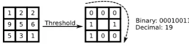
Local Binary Patterns (LBP) are a non-parametric method, that summarises local image structures efficiently by compar-ing each feature of the object with its neighbourcompar-ing features. The Local Binary Pattern (LBP) was introduced by Ojala et al. [15] [16] for describing 2D textures in still images. The most important properties of LBP for images are its tolerance regarding monotonic illumination changes and its computational simplicity. In the original definition, the LBP operator [15] assigns labels to image pixels by first comparing the 8 neighbours with the centre value (i.e., the neighbor pixel value is considered as 1 if its value is greater or equal to the central pixel value, and 0 otherwise), then considering the sequence of 1/0 in the pixel neighbourhood as a binary number. This is shown in Figure 1, where the upper left pixel in the neighbourhood is regarded as the most significant bit in the final code. This eight bit number encodes the mutual relationship between the gray levels of the central pixel and its
[image:3.595.330.524.111.159.2]neighbouring pixels. The histogram of the numbers obtained in such a way can then be used as a texture descriptor. This operator distinguished by its simplicity and its invariance to monotonic gray-level transformations.
Fig. 1. Computation of the basic LBP code from 3 x 3 neighbourhood of a central pixel. The central pixel is compared with each neighbour, starting from upper-left corner and produce 1 if its value is greater or equal, 0 otherwise. The result is an 8-bit binary code
LBP can be extended to operate on circular neighbourhoods of different radii, allowing sub-pixel alterations [16]. These initial formulations subsequently led to the definition of alter-native neighbourhood variants. For instance, Liao et al. [17] proposed oriented neighbourhood LBP which accounts for anisotropic information. Similarly the multi-block LBP(MB-LBP) that compares the averages of the gray level intensity of neighbouring pixels rather than the value of individual pixels, in order to capture macrostructural features in the image [18]. A more complete list and discussion on the many LBP variants can be found in [19].
C. Galois Field Algebra
A Galois Field is a finite field, i.e., a field in which there exists finitely many elements. For Galois Fields, the order of the field (i.e., the number of elements in the field) is always a prime or a power of a prime. For any prime integer p
and any integer m greater than or equal to 1, there is a unique field with pm elements denoted as GF(pm). These
finite fields are extensively used in cryptographic algorithms like Advanced Encryption Standard(AES), elliptical Curve Cryptography(ECC) as well as in coding theory like Reed Solomon codes. It is particularly useful in translating computer data as they are represented in binary forms. Representing data as a vector in a Galois field allows mathematical operations to scramble data easily and effectively. In this paper our goal is to use Galois field on the binary patterns obtained from the LBP when applied on a graph. Since our data is represented in the form of binary numbers, so we will assume our binary patterns are elements of GF(2m). As with any other field, the basic
operations are defined in Galois field. Two most commonly used operations are multiplicationandaddition.
Addition in Galois Fields:InGF(2m), addition is especially
easy, since addition and subtraction is the same, and further-more this operation can be done in hardware using basic XOR logic gate, since there is no concept of carry generation and carry propagation.
Multiplication in Galois Fields: In GF(2m), multiplication
polynomials over the same field. For example in the field of rational polynomialsQ[x](i.e., polynomialsf(x)with rational coefficients),f(x)is said to be irreducible if there do not exist two non-constant polynomialsg(x)andh(x)inxwith rational coefficients such that f(x) =g(x)h(x). A list of irreducible polynomials of degree 2 to 5 is given in Table I.
TABLE I
IRREDUCIBLE POLYNOMIALS OF DEGREES2THROUGH5
Degree irreducible polynomials
2 1 +x+x2
3 1 +x+x3,1 +x2+x3
4 1 +x+x4,1 +x+x2+x3+x4,1 +x3+x4
5
1 +x2+x5,1 +x+x2+x3+x5,1 +x3+x5, 1 +x+x3+x4+x5,1 +x2+x3+x4+x5, 1 +x+x2+x4+x5
III. GRAPHLBP
In this section we describe how LBP can be defined for a graph. We discuss the challenges that are involved in defining LBP on a graph and propose methods to overcome those problems. We refer the proposed framework as GraphLBP. We begin by defining LBP In its original form, the LBP operator assigns labels to image pixels by comparing the intensity value of a pixel with its 8 neighbours and is given by
LBP =
P−X1
p=0
s(gp−gc)2p,
wheregc is the gray value of the central pixel,gp is the gray
value of its neighbours andP is the total number of involved labels. The value of the function s(x) is 1 if x ≥ 0 and 0 otherwise.
In our approach, we define LBP for every vertex of a graph. For a labelled graph, where every vertex of a graph is assigned a unique label, comparison can be done directly (if there exists a partial ordering between lables). For unlabelled graphs, we use the degree of a vertex to construct LBP, i.e, the degree of a vertex is compared with the degree of its neighbour vertices. However, applying the LBP on graph-based representation is not a straight forward method because the graph-based representation has few limitations. First, there is no ordering information available in the vertices of a non-planner graph. This will result in different LBP for different ordering of neighbouring vertices. Secondly, the number of neighbours of a vertex are not fixed, resulting in LBP with varying lengths. Finally, graphs are sensitive to noise due to which there are additional/missing edges/vertices. For these reasons, applying LBP operator directly may not be practical.
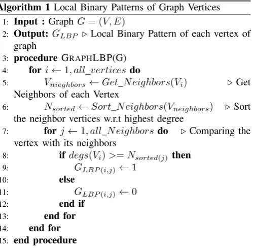
To overcome these problems, in this section we propose two algorithms, that together can be used to define GraphLBP. We begin by defining a LBP for a vertex of a graph. As mentioned earlier, we use the degree of a vertex to define its local binary pattern. To construct LBP for a vertex v, we take all the neighbours ofv and sort them in descending order according to their degrees. The pattern value for each vertex
[image:4.595.307.557.272.517.2]v is computed by comparing its degree with the degrees of its neighbour vertices and produce 1 if the deg(v) is greater or equal to the degree of its neighbour, otherwise 0. Consider, for example, the graph of Figure 2.
Fig. 2. A simple graph with 8 vertices
To construct a LBP for the vertexv in the graph of Figure 2, we take all its four neighbours and sort them into degree sequence order. The resulting sorted sequence is 6,4,4,3. Since deg(v) is 4, the LBP for the vertex v is 0111. This procedure is outlined in Algorithm 1.
Algorithm 1 Local Binary Patterns of Graph Vertices
1: Input :Graph G= (V, E)
2: Output: GLBP ⊲ Local Binary Pattern of each vertex of
graph
3: procedureGRAPHLBP(G)
4: fori←1, all vertices do
5: Vnieghbors←Get N eighbors(Vi) ⊲Get
Neighbors of each Vertex
6: Nsorted←Sort N eighbors(Vneighbors) ⊲ Sort
the neighbor vertices w.r.t highest degree
7: forj←1, all N eighbors do ⊲Comparing the
vertex with its neighbors
8: ifdegs(Vi)>=Nsorted(j)then
9: GLBP(i,j)←1
10: else
11: GLBP(i,j)←0
12: end if
13: end for 14: end for 15: end procedure
Note that the resulting binary pattern produced for a vertex
110. This value will be treated as the LBP of the vertex v. Note that this approach has two advantages. Firstly, it produces fixed length codes for each vertex. Secondly, it produces a more richer encoding by incorporating the information of the neighbours. The local binary patterns of the vertices are finally grouped using histogram binning to produce a global signature for graph characterization. Algorithm 2 outlines the steps performed in computing GraphLBP.
Algorithm 2 Features Extraction from Graph
1: Input : GraphGLBP, n
2: ⊲ The LBP computed in Algorithm 1 and bin size
3: Output: GraphV ector ⊲ Feature Vector of the Graph 4: procedure GETVECTOR(GLBP)
5: fori←1, all verticesdo
6: forj←1, all N eighborsdo
7: Vadd←gf add(GLBP(N eighborj), Vadd)
8: end for
9: Gvec(i)←gf deconv(Vadd, Pirreducible)
10: end for
11: Graphvector←hist(Gvec,10)
12: end procedure
Note that the Algorithm 2 requires two external parameters. In our experimental evaluation, we have chosen the irreducible polynomial1 +x+x3 of degree 3, while the number of bins as 10.
Time Analysis:The worst case running time of the GraphLBP (Algorithm 2) isO(|V|2). This is due to the fact that, in the
worst case(assuming complete graph), both the outer loop and the inner loop in the algorithm will be executed and will take
O(|V|2)of running time. For a graph, represented in the form
of adjacency list, the aggregate running time of the algorithm is O(|E|). Note that the running time of most state of the art algorithms including random walk, Ihara coefficients, and shape DNA isO(|V|3).
IV. EXPERIMENTALEVALUATION
In this section we perform experimental evaluation of the proposed method and compare it with state of the art methods. For this purpose, we selected the graphs that are extracted from different views of an object taken with various transformation and illumination conditions. The objective is to assess whether GraphLBP can be used to embed the graphs in a vector space to characterize their structure. The images are selected from
COIL (Columbia Object Image Library) [20]. This dataset consists of 20 different objects each with 72 views. These views are obtained from equally spaced directions over360o.
In our experiments we have selected 4 different objects with all their 72 views. Figure 3a shows some examples of photographs taken from COIL.
To construct graphs over these images, we have applied
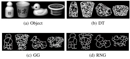
Harris corner detector[21]. Harris corner detector is used to extract a list of candidate feature points. We treat these feature points as vertices and construct a Delaunay triangulation over those feature points. A Delaunay triangulations (DT) [22]
for a set P of points in a Euclidean space is a triangulation, DT(P), such that no point in P is inside the circumcircle of any triangle in DT(P). Figure 3 shows an example of an object and its corresponding Delaunay Triangulation.
(a) Object (b) DT
[image:5.595.316.541.111.214.2](c) GG (d) RNG
Fig. 3. COIL Objects and their extracted Graphs
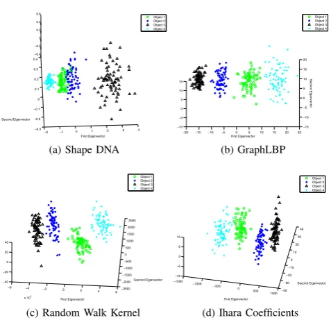
Once the graphs are extracted from the object images, we apply GraphLBP to the extracted graphs to embed them in a high-dimensional feature space. To evaluate the performance of the proposed method, we compare it with following state-of-the-art methods.
Random walk kernel [3]: Random walk kernel is state-of-the-art graph kernel used to compare graphs. It measures the similarity between two graphs by counting the frequencies of matching random walks in the two input graphs. It avoids the decomposition of the input graphs in to walks by using the product graph formalism. This increases the efficiency of the kernel.
shape DNA [23]: This method defines shape by a vector composed of first few smallest eigenvalues of the Laplacian matrix representation of a graph. This method was originally proposed by Reuter et al. [23] for 3D shape classification. For our experiments, we have chosen first ten positive eigenvalues of the Laplacian matrix. Note that the smallest eigenvalue of the Laplacian matrix is always zero and so we have ignored it in our representation.
Ihara coefficients [5]: This method uses a feature-vector that records prime cycle frequencies in a graph. These cycle frequencies are computed using first few coefficients of the reciprocal of the Ihara zeta function of the graph, commonly referred to as Ihara coefficients. For comparison purpose in our paper, we use the feature vector constructed from the coefficientsc3, c4andcln|2E|, as proposed by Peng in[5]. Note
that Ihara coefficients are considered a powerful tool to capture the cyclic structure of graphs [5], [24].
COIL dataset.
−2 −1 0 1 2 3 4 −0.3 −0.2 −0.1 0 0.1 0.2 0.3 0.4 −0.4 −0.2 0 0.2 0.4 0.6 First Eigenvector Second Eigenvector Object 1 Object 2 Object 3 Object 4
(a) Shape DNA
−20 −15 −10 −5 0 5 10 15 20 25 −15 −10 −5 0 5 10 15 20 −10 −5 0 5 10 15 Second Eigenvector First Eigenvector Object 1 Object 2 Object 3 Object 4 (b) GraphLBP
−6 −4 −2 0 2 4 6 x 10⁵
−2500 −2000 −1500 −1000 −500 0 500 1000 1500 2000 2500 −40 −20 0 20 40 Second Eigenvector First Eigenvector Object 1 Object 2 Object 3 Object 4
(c) Random Walk Kernel
−1500 −1000 −500 0
500 1000−40 −30 −20 −10 0 10 20 30 40 −10 −5 0 5 10 Second Eigenvector First Eigenvector Object 1 Object 2 Object 3 Object 4
[image:6.595.47.286.74.303.2](d) Ihara Coefficients
Fig. 4. PCA embedding of feature vectors computed from Delaunay Trian-gulations.
To quantitatively compare the performance of the proposed method with alternative methods, we cluster the graphs using
k-means clustering [25]. k-means clustering is a method, which aims to partition n observations intokclusters in which each observation belongs to the cluster with the nearest mean. We compute Rand index [26] of these clusters, which is a measure of the similarity between two data clusters. Table II compares the Rand indices of all the methods.
TABLE II
ACCURACIES OF DIFFERENT METHODS ONDELAUNAY TRIANGULATIONS
Method DT
GraphLBP 99.65%
Shape DNA 97.36%
Ihara 97.96%
Random Walk Kernel 97.99% Selected Ihara 98.97%
The above results show that GraphLBP can give better performance as compared to some state of the art methods.
To take this study one step further, we now apply GraphLBP to Gabriel graphs and relative neighbourhood graphs extracted from the same dataset. AGabriel Graph [27]for a set of n
points is a subset of Delaunay triangulation, which connects two data points vi and vj for which there is no other point
vk inside the open ball whose diameter is the edge (vi, vj).
The relative neighbourhood graph [28] is also a subset of Delaunay Triangulation. In this case a lune is constructed on each Delaunay edge. The circles enclosing the lune have their centres at the end-points of the Delaunay edge; each circle has a radius equal to the length of the edge. If the lune contains another node then its defining edge is pruned from the relative neighbourhood graph. Figure 3c and 3d show an example of a
Gabriel Graph and a relative neighbourhood graph respectively for corresponding images shown in Figure 3a. Note that, since both the GG and RNG are subset of DT, the experiments on those datasets allow us to investigate the performance of the proposed method under controlled structural modification.
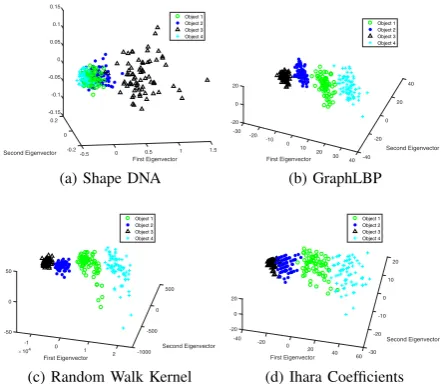
As with DT, we apply GraphLBP and alternate methods to the graphs extracted from the same objects and embed the resulting feature vectors in a three dimensional vector space using PCA. Figure 5 shows the resulting embeddings of the feature vectors extracted from Gabriel graphs, while Figure 6 shows the resulting embeddings of the feature vectors extracted from Relative neighbourhood graphs. For compari-son purpose, we have shown the visualisation results for the proposed method and the alternate methods.
−1 −0.5 0 0.5 1 1.5 2 2.5 −0.2 −0.15 −0.1 −0.05 0 0.05 0.1 0.15 0.2 −0.2 −0.15 −0.1 −0.05 0 0.05 0.1
0.15 Second Eigenvector
First Eigenvector
Object 1 Object 2 Object 3 Object 4
(a) Shape DNA
−20 −15−10 −5 0 5 10 15 20 25 30 −15 −10 −5 0 5 10 15 −10 −5 0 5 10 15 Second Eigenvector First Eigenvector Object 1 Object 2 Object 3 Object 4 (b) GraphLBP −2 −1 0 1 2 3 x 10⁵
−4000 −3000 −2000 −1000 0 1000 2000 3000 −1000 100 Second Eigenvector First Eigenvector Object 1 Object 2 Object 3 Object 4
(c) Random Walk Kernel
−400 −300 −200 −100 0 100 200 300 −50 −40 −30 −20 −10 0 10 20 30 40 −20 −10 0 10 20 First Eigenvector Second Eigenvector Object 1 Object 2 Object 3 Object 4
(d) Ihara Coefficients
Fig. 5. PCA embedding of feature vectors computed from Gabriel graphs.
The embedding results of Figure 5 suggest that, under controlled structural modification, GraphLBP can still provide a better separation as compared to other state of the art methods. To quantitatively evaluate the performance of the proposed method, we compute the Rand index of the resulting clusters. Table III reports the resulting Rand indices for the proposed method and alternative methods.
TABLE III
ACCURACIES OF DIFFERENT METHODS ONGABRIEL GRAPHS
Method GG RNG
GraphLBP 99.65% 98.30%
Shape DNA 71.66% 75.06%
Ihara 82.31% 64.97%
Random Walk Kernel 93.27% 95.66% Selected Ihara 93.85% 95.34%
-0.15 -0.1 -0.05 0
0.2 0.05 0.1 0.15
Second Eigenvector 0
First Eigenvector -0.2-0.5 0 0.5 1 1.5
Object 1 Object 2 Object 3 Object 4
(a) Shape DNA
40
20
Second Eigenvector 0 -20
-30
-20 -10 -20
First Eigenvector 0
10 20
30 -40 40 0
20
Object 1 Object 2 Object 3 Object 4
(b) GraphLBP
500
0
Second Eigenvector -500 -50
-1 104
First Eigenvector 0
1 2 -1000 0
50
Object 1 Object 2 Object 3 Object 4
(c) Random Walk Kernel
20
10
0
Second Eigenvector -10 -20
-20 -40
-20 First Eigenvector
0 20 40 -30 60 0
20
Object 1 Object 2 Object 3 Object 4
[image:7.595.55.276.54.246.2](d) Ihara Coefficients
Fig. 6. PCA embedding of feature vectors computed from relative neighbour-hood graphs.
V. CONCLUSION
In this paper we have described Graph-LBP. This is a novel framework for characterizing graphs extracted from both real world and synthetic data. The proposed method is scaleable and maintains the simplicity and elegance characteristics of original pixel LBP, which can be used to construct the fea-ture vectors from image texfea-tures. We provided a route for extracting structural properties from graphs via LBP, and have mapped them to a vector space using Galois field algebra. Our future research directions will focus on a) expanding our method to other datasets i.e. ALOI, ETHZ etc. b) encompass weighted graphs, directed graphs and hyper graphs - so that it can be extended to develop more general object represen-tations, and c) expand of idea of Graph-LBP on 3D mesh models.
REFERENCES
[1] H. Bunke, “On a relation between graph edit distance and maximum common subgraph,”Pattern Recognition Letters, vol. 18, no. 8, pp. 689– 694, 1997.
[2] A. Dutta and H. Sahbi, “High order stochastic graphlet embedding for graph-based pattern recognition,”arXiv:1702.00156, 2017.
[3] T. G¨artner, P. Flach, and S. Wrobel, “On graph kernels: Hardness results and efficient alternatives,” in Learning Theory and Kernel Machines. Springer, 2003, pp. 129–143.
[4] K. M. Borgwardt and H.-P. Kriegel, “Shortest-path kernels on graphs,”
inData Mining, Fifth IEEE International Conference on. IEEE, 2005,
pp. 8–pp.
[5] P. Ren, R. C. Wilson, and E. R. Hancock, “Graph characterization via ihara coefficients,” IEEE Transactions on Neural Networks, vol. 22, no. 2, pp. 233–245, 2011.
[6] J. Qiangrong, L. Hualan, and G. Yuan, “Cycle kernel based on spanning tree,” in Electrical and Control Engineering (ICECE), 2010
Interna-tional Conference on. IEEE, 2010, pp. 656–659.
[7] E. Hancock, “Spectral approaches to learning in the graph domain,” in
Proceedings of the 2010 Workshop on Graph-based Methods for Natural
Language Processing. Association for Computational Linguistics, 2010,
pp. 47–47.
[8] J. Sun, M. Ovsjanikov, and L. Guibas, “A concise and provably infor-mative multi-scale signature based on heat diffusion,” Comp. Grarph
Forum, pp. 1383–1392, 2010.
[9] T. Ojala, M. Pietikainen, and D. Harwood, “Performance evaluation of texture measures with classification based on kullback discrimination of distributions,” inProceedings of 12th International Conference on
Pattern Recognition, vol. 1, 1994, pp. 582–585 vol.1.
[10] C. Song, F. Yang, and P. Li, “Rotation invariant texture measured by local binary pattern for remote sensing image classification,” in
Education Technology and Computer Science (ETCS), 2010 Second
International Workshop on, vol. 3. IEEE, 2010, pp. 3–6.
[11] Z. Guo, L. Zhang, and D. Zhang, “Rotation invariant texture clas-sification using lbp variance (lbpv) with global matching,” Pattern
recognition, vol. 43, no. 3, pp. 706–719, 2010.
[12] D. Huang, C. Shan, M. Ardabilian, Y. Wang, and L. Chen, “Local binary patterns and its application to facial image analysis: a survey,”IEEE Transactions on Systems, Man, and Cybernetics, Part C (Applications
and Reviews), vol. 41, no. 6, pp. 765–781, 2011.
[13] L. Cai, C. Ge, Y.-M. Zhao, and X. Yang, “Fast tracking of object contour based on color and texture,”International Journal of Pattern Recognition
and Artificial Intelligence, vol. 23, no. 07, pp. 1421–1438, 2009.
[14] N. Werghi, S. Berretti, and A. Del Bimbo, “The mesh-lbp: a framework for extracting local binary patterns from discrete manifolds,” IEEE
Transactions on Image Processing, vol. 24, no. 1, pp. 220–235, 2015.
[15] T. Ojala, M. Pietik¨ainen, and D. Harwood, “A comparative study of texture measures with classification based on featured distributions,”
Pattern recognition, vol. 29, no. 1, pp. 51–59, 1996.
[16] T. Ojala, M. Pietikainen, and T. Maenpaa, “Multiresolution gray-scale and rotation invariant texture classification with local binary patterns,”
IEEE Transactions on pattern analysis and machine intelligence, vol. 24,
no. 7, pp. 971–987, 2002.
[17] S. Liao and A. C. Chung, “Face recognition by using elongated local binary patterns with average maximum distance gradient magnitude,” in
Asian conference on computer vision. Springer, 2007, pp. 672–679.
[18] L. Zhang, R. Chu, S. Xiang, S. Liao, and S. Z. Li, “Face detection based on multi-block lbp representation,” inInternational Conference
on Biometrics. Springer, 2007, pp. 11–18.
[19] M. Pietik¨ainen, A. Hadid, G. Zhao, and T. Ahonen,Computer vision
using local binary patterns. Springer Science & Business Media, 2011,
vol. 40.
[20] S. A. Nene, S. K. Nayar, H. Murase et al., “Columbia object image library (coil-20),” Technical report CUCS-005-96, Tech. Rep., 1996. [21] C. Harris and M. Stephens, “A combined corner and edge detector.” in
Alvey vision conference, vol. 15. Citeseer, 1988, p. 50.
[22] B. Delaunay, “Sur la sph´ere vide,” Izvestia Akademii Nauk SSSR,
Otdelenie Matematicheskikh i Estestvennykh Nauk, pp. 793–800, 1934.
[23] M. Reuter, F.-E. Wolter, and N. Peinecke, “Laplacebeltrami spectra as shape-dna of surfaces and solids,” Computer-Aided Design, vol. 38, no. 4, pp. 342 – 366, 2006.
[24] F. Aziz, R. C. Wilson, and E. R. Hancock, “Backtrackless walks on a graph,”IEEE transactions on neural networks and learning systems, vol. 24, no. 6, pp. 977–989, 2013.
[25] J. B. MacQueen, “Some methods for classification and analysis of multivariate observations,” inProc. of the fifth Berkeley Symposium on
Mathematical Statistics and Probability, vol. 1. University of California
Press, 1967, pp. 281–297.
[26] W. M. Rand, “Objective criteria for the evaluation of clustering meth-ods,”Journal of the American Statistical Association, vol. 66, no. 336, pp. 846–850, 1971.
[27] K. R. Gabriel and R. R. Sokal, “A new statistical approach to geographic variation analysis,”Systematic Zoology, pp. 205–222, 1969.