Thermal Safe Test Scheduling for Core Based System on a Chip Integrated Circuits

Thermal-Safe Test Scheduling for Core-Based System-on-Chip Integrated

Circuits

Paul Rosinger, Bashir M. Al-Hashimi University of Southampton

School of Electronics and Computer Science Southampton, SO17 1BJ, UK

{pmr,bmah}@ecs.soton.ac.uk

Krishnendu Chakrabarty

Department of Electrical and Computer Engineering Duke University

Durham, NC 27708 [email protected]

Abstract

Overheating has been acknowledged as a major problem during the testing of complex system-on-chip (SOC) integrated circuits. Several power-constrained test scheduling solutions have been recently proposed to tackle this problem during system integration. However, we show that these approaches cannot guarantee hot-spot-free test schedules because they do not take into account the non-uniform distribution of heat dissipation across the die and the physical adjacency of simultaneously active cores. This paper proposes a new test scheduling approach that is able to produce short test schedules and guarantee thermal-safety at the same time. Two thermal-safe test scheduling algorithms are proposed. The first algorithm computes an exact (shortest) test schedule that is guaranteed to satisfy a given maximum temperature constraint. The second algorithm is a heuristic intended for complex systems with a large number of embedded cores, for which the exact thermal-safe test scheduling algorithm may not be feasible. Based on a low-complexity test session thermal cost model, this algorithm produces near-optimal length test schedules with significantly less computational effort compared to the optimal algorithm.

1. Introduction

Recent reports from industry indicate that power consumption during scan testing in some designs can be significantly higher compared to the normal operation mode. A case study involving the Motorola Version 3 ColdFire processor [14] reported a minimum of 3X increase of test power over functional power. In the same experiment, there have been also cases where test power for at-speed compressed patterns was as high as 8X the functional power. A more recent industrial article [19] reports test power up to 30X higher compared to the normal operation mode. The elevated levels of power dissipation during test lead inherently to higher die temperatures compared to the normal operation. This creates a number of problems, because both soft error rates and aging increase exponentially with temperature. An undesirable consequence of overheating is thermal stress. At high temperatures, transistors fail to switch properly and many failure mechanisms, such as electro-migration, are accelerated resulting in an overall decrease in reliability or even permanent damage. These problems are exacerbated for core-based system-on-chip (SOC) designs because, quite often, several embedded cores are tested concurrently in order to reduce the overall test time. A significant amount of research has been devoted to reducing power consumption during test in order to avoid the overheating of the silicon die during test. Consequently, several low power solutions targeting core-level design-for-test(DFT), as well as system-level DFT have been recently proposed. Techniques falling in the first category include low-power scan chain architectures with gated clocks [18, 17], scan cell and test pattern reordering [3, 5], and low-transition test patterns generated by specialised ATPG algorithms [22] and low-transition TPGs [21]. The second category of techniques is mainly based on power-constrained test scheduling algorithms [2, 9, 11, 7, 6, 1, 15, 12, 13]1_.

This paper focuses on avoiding overheating during test through appropriate test scheduling. The main contri-butions of the paper are

• propose thermal-aware test as a better alternative to power-constrained test when dealing with overheating during test

• propose a test session thermal model which will reduce the thermal simulation effort required to identify a thermal-safe test schedule

The motivation for this work is presented in Section 2. The basic ideas behind the existing power constrained test scheduling approaches are examined from the perspective of chip overheating, and it is explained why these approaches cannot guarantee thermal-safety. Section 3 proposes a new test scheduling approach that overcomes this problem. An exact algorithm that guarantees minimum test times as well as thermal-safety is presented in

1_{It should be noted that in reference [13], the term “hot-spot” is used to denote an area of the die where the peak power consumption}

Section 3.1. It is shown through experimental results that significantly shorter test schedules can be obtained without increasing the maximum die temperature during test when compared with existing power-constrained test scheduling approaches. While this algorithm guarantees the optimal solution for a given thermal limit, it may require significant computational effort for complex systems, mainly due to the required amount of accurate thermal simulations. Therefore, a fast heuristic algorithm for thermal-aware test scheduling is proposed Section 3.3. This approach uses a low-complexity test session thermal cost model in order to speed-up the solution space exploration and reduce the thermal simulation effort required to reach an acceptable solution. The experiments show that this heuristic produces nearly-optimal test schedules (and even optimal schedules in some cases) while significantly reducing the thermal simulation effort.

2. Motivation

In this section, we examine the effectiveness of power-constrained test scheduling(PCTS) as a means of avoiding die overheating during test. The common idea behind PCTS is to impose a chip-wide maximum allowable limit on power consumption, which should not be exceeded during test application. Several recently proposed power-constrained test scheduling algorithms aim to maximise the number of tests running in parallel without exceeding this limit [2, 9, 11, 7, 6, 1, 15, 12, 13].

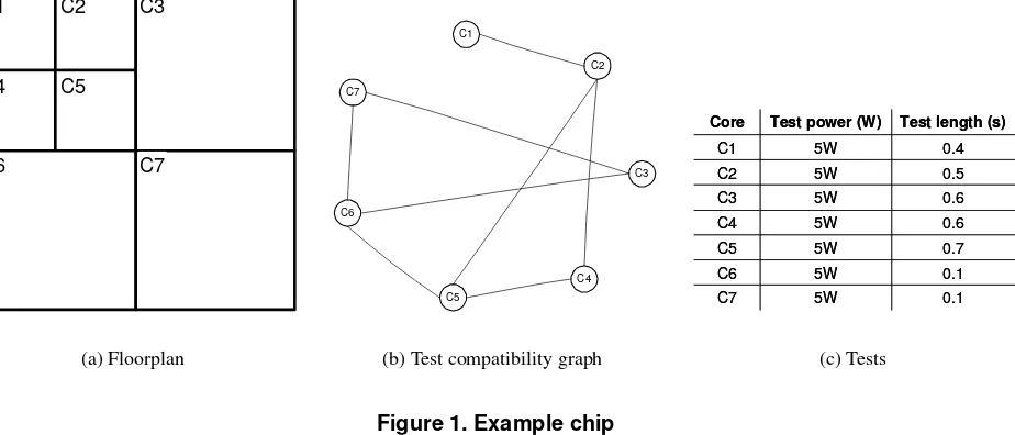
C1 C2 C4 C5 C3 C6 C7 (a) Floorplan C1 C2 C7 C3 C5 C4 C6

(b) Test compatibility graph

0.5 5W C2 0.6 5W C3 0.6 5W C4 0.7 5W C5 0.1 5W C6 0.1 5W C7 0.4 5W C1

Test length (s) Test power (W)

Core 0.5 5W C2 0.6 5W C3 0.6 5W C4 0.7 5W C5 0.1 5W C6 0.1 5W C7 0.4 5W C1

Test length (s) Test power (W)

Core

(c) Tests

Figure 1. Example chip

is 4 times higher than that of C3). Moreover, the hottest cores in the two test sessions were C5 and C7. This is because of their reduced lateral heat removal paths: cores C5 and C7 have only 2 “cold” (inactive) neighbours (more specifically, on their “EAST” and “SOUTH” edges), while all other cores have 3 “cold” neighbours.

This example has shown that imposing a global power constraint during test cannot guarantee thermal-safety because it does not consider power densities across the die nor the clustering of “hot” cores, which can limit the lateral heat removal. In the following section, we present a new test scheduling approach which overcomes these issues.

3. Thermal-safe test scheduling

The mean time to failure (MTTF)—a commonly used metric in reliability models—is based on the Arrhe-nius equation, which shows that reliability is decreasing exponentially with the absolute junction temperature:

M T T F = AeEakT, whereAis an empirical constant, E_a is the so-called activation energy andk is Boltzmann’s

In the following, we propose two thermal-safe test scheduling algorithms. The first one, although computation-ally expensive, computes the exact solution to the problem, i.e., the shortest test schedule that meets the thermal constraint. The second proposed algorithm takes into consideration the on-chip lateral heat transfer paths in order to determine a nearly-optimal solution with less computational effort. The results obtained using this algorithm are then compared with the solutions obtained using the exact algorithm.

Both proposed test scheduling algorithms start from the set of cores (S) of the target system, the corresponding test compatibility graph (TCG), such as the one shown in Figure 1(b), and the maximum junction temperature that can be tolerated during test (Tmax). Each core is annotated with the length of its corresponding test. The TCG

cap-tures the concurrency compatibility relationships between the system cores: each node in the TCG corresponds to a core, and an edge between two nodes means that the two corresponding cores can be tested concurrently without causing any resource conflicts. The floorplan of each system is also needed for performing thermal simulations on the generated test sessions. The algorithms return a thermal-safe test schedule as a list of test sessions, where each test session is a group of cores to be tested concurrently.

3.1. The exact algorithm

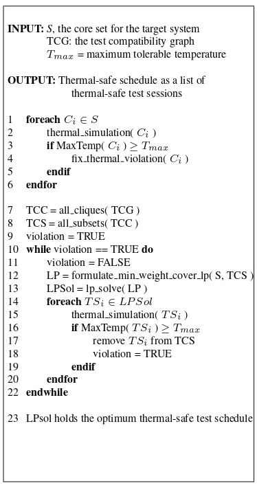
In this subsection we present an algorithm for determining an exact solution to the thermal-safe test scheduling problem (see Figure 2). The algorithm computes the shortest test schedule which guarantees that the specified

Tmaxwill not be exceeded during test. An outline of this algorithm is presented in the following. First, a thermal

simulation is performed on each individual core and corresponding test in order to ensure they all comply with the thermal constraint. the shortest test schedule is computed using only the test compatibility relations between the cores. A thermal simulation is then performed to check whether the test schedule complies with the thermal constraint (Tmax). IfTmaxis violated during any test sessions, these test sessions are discarded and the process is

repeated until a thermal-safe test schedule is found.

[C2,C1], [C3,C6,C7]]. Since the number of nodes in TCG (number of cores in a design) is reasonably low, we have used a straight-forward exhaustive search algorithm for determining TCC (the all cliques function in Figure 2 ). Each clique in the TCC represents a maximal group of cores that can be tested concurrently without causing resource sharing conflicts. Consequently, any valid test schedule must consist only of subsets (TCS) of the cliques in TCC (line 8 in Figure 2). The shortest test schedule can be determined as the minimum weight set cover for TCS, where the weight of each test compatible subset in TCS is the length of its longest test (it is assumed that all tests in a test session start at the same time). For our example, TCS and the corresponding subset weights is [C2]=0.5, [C2, C5, C4]=0.7, [C5]=0.7, [C5, C6]=0.7, [C2, C5]=0.7, [C3]=0.6, [C7, C3]=0.6, [C4]=0.6, [C2, C4]=0.6, [C5, C4]=0.7, [C3, C6]=0.6, [C7, C6]=0.1, [C7]=0.1, [C2, C1]=0.5, [C1]=0.4, [C7, C3, C6]=0.6, [C6]=0.1 The minimum weight set cover is determined using a O-1 integer linear programming (ILP) formulation (theformulate min weight cover lpfunction in Figure 2). The ILP formulation for our example is shown below:

Constraint 1:XT CS0+XT CS1+XT CS4 +XT CS8 +XT CS13 = 1

Constraint 2:XT CS1+XT CS2+XT CS3 +XT CS4+XT CS9 = 1

Constraint 3:XT CS6+XT CS11+XT CS12+XT CS15= 1

Constraint 4:XT CS5+XT CS6 +XT CS10+XT CS15 = 1

Constraint 5:XT CS13+XT CS14 = 1

Constraint 6:XT CS1+XT CS7 +XT CS8 +XT CS9 = 1

Constraint 7:XT CS3+XT CS10+XT CS11+XT CS15+XT CS16 = 1

Minimise: 0.5XT CS0 + 0.7XT CS1 + 0.7XT CS2 + 0.7XT CS3 + 0.7XT CS4 +0.6XT CS5 + 0.6XT CS6+ 0.6XT CS7 + 0.6XT CS8

+0.7XT CS9 + 0.6XT CS10+ 0.1XT CS11 + 0.1XT CS12

+0.5XT CS13 + 0.4XT CS14+ 0.6XT CS15+ 0.1XT CS16

A value of 1 for the binary variable XT CSi , means T CSi represents a test session in the final test schedule, and a value of 0 if it does not. A constraint is added to the ILP formulation for each coreCi, hence 7 constraints

for our example, enforcing that each core should be covered by one and only one TCS in the final solution. The ILP objective is to minimise the sum of the weights (in this case the test lengths) of the test compatible subsets in the minimum weight set cover. The solution for this particular ILP is XT CS1 = 1, XT CS14 = 1

and XT CS15 = 1. The corresponding test schedule will be [[C2, C5, C4],[C1],[C7, C3, C6]]. Once a valid test

schedule has been computed, a thermal simulation is performed to check whetherTmaxis not exceeded during test.

step. The maximum temperature for each core can then be easily computed from these traces. Thermal simulations for the three test sessions in the previously computed test schedule produce the following results:

Test session [C2,C4,C5] [C1] [C3,C6,C7]

Max temperature (°C) 127.19 98.83 66.47

These results show that the maximum die temperature during the first test session([C2,C5,C4]) violates the thermal constraint of 110 °C(line 16). Consequently, this test session is removed from TCS and a new test schedule is computed based on the updated TCS. The algorithm continues until a test schedule which does not violate the thermal constraint is found. For our example, the shortest thermal-safe test schedule is found after three such iterations and it consists of the following test sessions:

Test session [C2,C4] [C5] [C1] [C3,C6,C7]

Max temperature (°C) 103.2 106.54 98.83 66.47

In order to reach this result, a total of 5.8 seconds of test session time had to be thermally simulated.

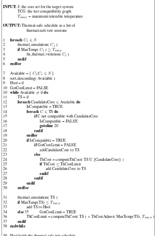
INPUT:S, the core set for the target system

TCG: the test compatibility graph

Tmax= maximum tolerable temperature

OUTPUT:Thermal-safe schedule as a list of

thermal-safe test sessions

1 foreachCi∈S

2 thermal simulation(Ci)

3 ifMaxTemp(Ci)≥Tmax

4 fix thermal violation(Ci)

5 endif

6 endfor

7 TCC = all cliques( TCG ) 8 TCS = all subsets( TCC ) 9 violation = TRUE

10 whileviolation == TRUEdo

11 violation = FALSE

12 LP = formulate min weight cover lp( S, TCS ) 13 LPSol = lp solve( LP )

14 foreachT Si∈LP Sol

15 thermal simulation(T Si)

16 ifMaxTemp(T Si)≥Tmax

17 removeT Sifrom TCS

18 violation = TRUE

19 endif

20 endfor

22 endwhile

23 LPsol holds the optimum thermal-safe test schedule

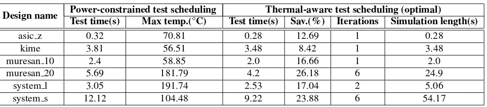
3.2. Experimental results for the exact algorithm

Design name Power-constrained test scheduling_{Test time(s) Max temp.(°C) Test time(s) Sav.(%) Iterations Simulation length(s)}Thermal-aware test scheduling (optimal)

asic z 0.32 70.81 0.28 12.69 1 0.28

kime 3.81 56.51 3.48 8.42 1 3.48

muresan 10 2.4 58.85 2.0 16.66 1 2.0

muresan 20 5.69 181.79 4.2 26.18 6 24.9

system l 3.05 191.74 2.53 17.04 2 5.06

system s 12.12 104.48 9.22 23.88 6 54.17

Table 1. Power-constrained test scheduling vs. optimal thermal-aware test scheduling

Table 1 compares the results obtained using the proposed algorithm with those obtained using the power con-strained test scheduling approach presented in [7]. We have chosen the approach presented in [7] for comparison since it is very recent, has been applied to large designs and performs well in comparison with other existing power constrained test scheduling approaches. Details such as floorplan information and realistic test power and time values had to be added or modified in the original design descriptions in order to provide all necessary in-formation for the proposed thermal safe test scheduling algorithms. The modified design descriptions used in our experiments can be found at [16]. Some of the physical constants used for thermal simulations performed with the HotSpot tool presented in [20] are reported in Table 4. The second column shows the test times corresponding to the power-constrained test schedules. Columns 4 to 7 show the results corresponding to the proposed thermal-aware test scheduling algorithm. For each design, the temperature limitTmaxwas set to the maximum temperature

under one second of CPU time on a Pentium IV @ 1.8GHz system.

3.3. Heuristic algorithm

Although the algorithm presented in the previous section computes the optimal solution to the thermal-safe test scheduling problem, it requires significant computational effort, especially because it requires a large amount of thermal simulations. This is mainly because no knowledge of the heat transfer paths is used while computing the test schedule and the thermal compliance check is performed only in a post-scheduling phase. This implies that for tight thermal constraints (such as in the case ofsystem sshown in Table 1), several iterations, and thus several thermal simulation runs, are required until a valid solution is found. The thermal simulation effort required to identify thermal-safe test schedules can be reduced by exploiting the knowledge of the on-chip heat transfer paths. There are two predominant paths for heat transfer out of the integrated circuit package. The first one is from the die to the surrounding package material, then to the package lead frame and on to the printed circuit board, and finally to the ambient air. The second path is from the package to the heat spreader to the heat sink and then to the ambient air. Local die temperature is strongly dependent on the proximity with other heat sources because close heat sources means more heat has to flow through the same paths. Therefore, keeping simultaneous heat sources as far apart as possible reduces the probability of hot-spots.

In order to capture the thermal interactions between different cores that are tested concurrently, we have derived a thermo-resistive model for the test sessions. The basic idea is to derive some quantitative measure of the lateral heat removal paths for a core by taking into account the thermal interactions with active neighbouring cores.

The duality between the electrical and thermal domains, illustrated in Table 2, offers a convenient basis for an architecture-level thermal model. According to this duality relationship, heat flow can be described as a “current” passing through a thermal resistance, leading to a temperature difference analogous to a “voltage”. Thermal resistanceRthis directly proportional to the thickness of the material (t) and inversely proportional to the

cross-sectional area across which the heat is being transfered (A):

Rth= t

kA (1)

wherek is the thermal conductivity of the material per volume unit (100W/mK for silicon and 400W/mK for

copper at 85°C).

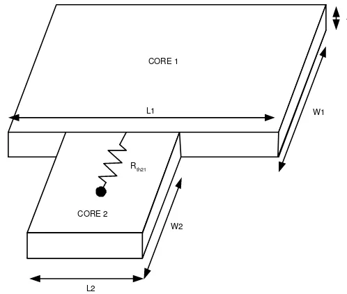
In order to clarify how the lateral thermal resistances are computed, consider the two adjacent cores CORE1 and CORE2 shown in Figure 3. The chip thickness is t and the core dimensions are (L1,W1) and (L2, W2)

respectively. The lateral resistanceRth21is the thermal resistance from the centre of Block 2 to the shared edge of

Thermal domain Electrical domain

P, heat flow, power (W) I, current flow (A) T, temperature difference (K) V, voltage (V)

Rth, thermal resistance (K/W) R, electrical resistance (Ω)

Table 2. The duality between the thermal and electrical domains

and L2*t . The constriction thermal resistance can be calculated by assuming the heat source area to be L1*t , the silicon bulk area that accepts the heat to be L2*t , and the thickness of the bulk to be W2/2. With these values found, the spreading/constriction resistance can be computed using the formulas given in [8]. The resistance is of the spreading type if the lateral area of the source is smaller than the bulk lateral area, and it is of the constriction type otherwise. When computing lateral thermal resistances, each core is assumed to present a thermal resistance towards each neighbouring core.

L2

W2

L1 W1

Rth21

CORE 1

CORE 2

t

Figure 3. Lateral thermal resistance between neighbouring cores

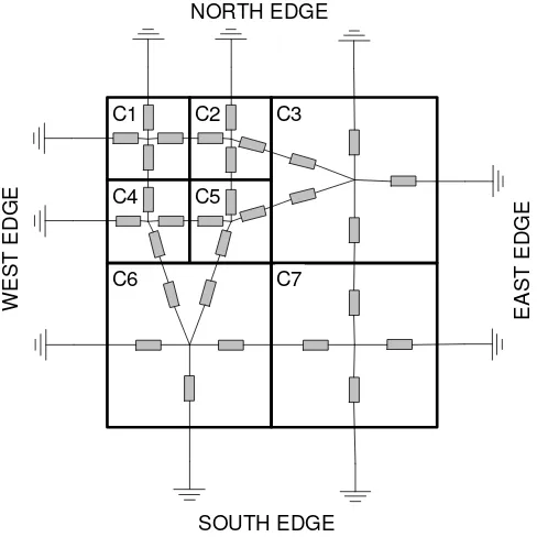
The lateral thermo-resistive representation for the example floorplan system shown in Figure 1(a) according to the thermo-resistive model thermal model presented in [20], is shown in Figure 4. In the following we are proposing a test session thermal cost model aiming to capture the thermal effects due to the physical proximity of simultaneously active cores, since these effects can be controlled by the choice of cores that are to be active at the same time. The proposed test session thermal cost model is derived from this lateral thermo-resistive model presented using the following simplifying assumptions:

2. The heat transfer between two cores tested concurrently is considered to be negligible, hence the thermal resistance between those cores is ignored for the current test session. This is a valid assumption because the amount of exchanged heat depends on the temperature difference, which is low for cores tested at the same time.

3. Inactive cores are assumed to be thermally grounded, i.e. their temperature is assumed to be equal to the ambient temperature and fixed for the entire duration of the test session.

C1 C2

C4 C5

C3

C6 C7

W

E

S

T

E

D

G

E

E

A

S

T

E

D

G

E

SOUTH EDGE NORTH EDGE

Figure 4. Lateral thermo-resistive model

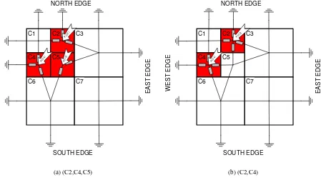
C1 C2 C4 C5 C3 C6 C7 W E S T E D G E E A S T E D G E SOUTH EDGE NORTH EDGE P(C 4) P(C 2) P(C 5) (a) (C2,C4,C5) C1 C2 C4 C5 C3 C6 C7 W E S T E D G E E A S T E D G E SOUTH EDGE NORTH EDGE P(C 4) P(C2 ) (b) (C2,C4)

Figure 5. Lateral thermo-resistive models for two test sessions

associated with an active core represents good heat exchange between the core and the ambient, consequently it predicts a lower core temperature during test. On the other hand, a large lateral thermal spreading resistance means poor heat exchange with the ambient, therefore it signals a potential hot-spot during test for cores with high power consumption. This can be seen by comparing the lateral thermo-resistive models shown in Figure 3.3. Each active core in Figure 5(a) has only three lateral heat removal paths, represented by three thermal resistors. Cores C2 and C4 shown in Figure 5(b) have both gained an additional lateral heat removal path through the removal of core C5 from the test session. The equivalent lateral thermal resistances of cores C2 and C4 is lower in this case compared to the scenario for test session [C2,C4,C5] shown in Figure 5(a). Thermal simulations performed on the two test sessions shown in Figure 3.3 yielded a 103.20 °C maximum temperature for [C2,C4] and a 127.19 °C maximum temperature for [C2,C4,C5], which supports our earlier observations.

The thermal cost model we are proposing for a core is basically the value of the equivalent thermal resistance towards cooler surroundings weighted by the power dissipated by that core, as shown in Equation 2. This is necessary in order to account for the actual power density of the core as well as for the lateral heat removal paths.

T hCost(Ci, T S) =Rth(Ci, T S)×P(Ci), Ci ∈T S (2)

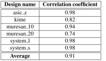
computed its thermal cost according to Equation 2, and the worst-case (i.e. maximum) values were correlated with the maximum temperature reached during the execution of each test session. The high correlation coefficients obtained for several designs, shown in Table 3, suggest that lateral heat spreading has a significant influence on the maximum core temperature. The maximum core temperature during test was determined through thermal simulations using the HotSpot tool [20].

Design name Correlation coefficient

asic z 0.98

kime 0.82

muresan 10 0.94

muresan 20 0.74

system l 0.98

system s 0.98

Average 0.91

Table 3. Correlation between the test session thermal cost and maximum core temperature

Based on the results of the previous experiment, we are extending our thermal cost model to test sessions as follows:

T hCost(T S) = maxT hCost(Ci, T S), Ci∈T S (3)

cost of TS, scaled down linearly by the fraction by which Tmax was exceeded. The thermal cost adjustment factor is computed as follows:

T hCostAdjust(M axT emp(T S), Tmax) = (M axT emp(T S)−Tmax)

Tmax ×

K+ 1 (4)

where K ∈ (0,1] is a user specified constant used to relax the thermal cost limit (ThCostLimit). In our experiments, we have usedK= 0.5. Once a thermal cost limit had been computed, a core is added to the current test session only if does not increase the test session thermal cost over ThCostLimit (lines 23-38). This way, it is ensured that once a thermal violation has been detected, test sessions with similar or worse lateral heat exchange capabilities are avoided without requiring lengthy thermal simulations.

We are illustrating the steps of this algorithm using the example system shown in Figure 2. The same thermal constraint Tmax = 100 °C used for the exact algorithm in Section 3.1 will be used here as well. After the initial core check, theAvailablearray is initialised with all cores in the system arranged in the descending order of their test lengths (Line 7):

Available= [C5, C3, C4, C2, C1, C6, C7] (5)

=[C5], and TS is added to the test schedule and removed from the available cores since it’s maximum temperature of 106.54 °C meets the thermal constraint. The GotCostLimit is set to FALSE, and the algorithm continues to schedule the remaining cores. In the next iterations, the algorithm adds [C3,C6,C7], [C2,C4] and [C1] to the test schedule. This matches the test schedule produced by the exact algorithm, however the thermal simulation effort was reduced from 5.8 seconds of test session time to 3.7 seconds. The complexity of computing a test session using this approach isO(N3), where N is the number of cores. However, the thermal simulation (line 31 in Figure 6), which is the most computationally expensive part of the algorithm is performed in the outer-most loop, which has only a complexity ofO(N). This is a considerable improvement in terms of the required computational effort over the exact algorithm described in Section 3.1, which has exponential complexity due to the NP-hard nature of the optimisation problem.

3.4. Experimental results for the heuristic algorithm

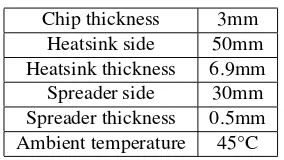
Chip thickness 3mm Heatsink side 50mm Heatsink thickness 6.9mm Spreader side 30mm Spreader thickness 0.5mm Ambient temperature 45°C

Table 4. Chip physical constants

A number of experiments have been performed in order to assess the performance of the proposed test schedul-ing heuristic. The first set of experiments were used to compare the proposed heuristic with the power-constrained test scheduling approach presented in [7]. The results of these experiments are reported in Table 5. The maximum temperature during test corresponding to the power constrained test schedules was used as a thermal constraint (Tmax) for the proposed test scheduling algorithm. This way, it is guaranteed that the resulting test schedules will

not lead to higher temperatures than that using the power-constrained approach. From the 4th and 5th columns, it can be observed that the proposed heuristic algorithm outperformed the power-constrained test scheduling ap-proach for all designs, producing up to 24% shorter test schedules. Moreover, for 3 out of the 6 designs considered, the heuristic algorithm produced the same test schedules as the exact algorithm presented in Section 3.1. The last column in Table 5 shows significant reductions in terms of thermal simulation effort when compared to the exact algorithm. For example, the simulation length was reduced from 54 seconds to 18 seconds forsystem s.

INPUT:S, the core set for the target system TCG: the test compatibility graph

Tmax= maximum tolerable temperature

OUTPUT:Thermal-safe schedule as a list of

thermal-safe test sessions

1 foreachCi∈S

2 thermal simulation(Ci)

3 ifMaxTemp(Ci)≥Tmax

4 fix thermal violation(Ci)

5 endif

6 endfor

7 Available ={Ci|Ci∈S}

8 sort descending( Available ) 9 Hsol =∅

10 GotCostLimit = FALSE

10 whileAvailable6=∅do

11 TS =∅

12 foreachCandidateCore∈Availabledo

13 IsCompatible = TRUE

14 foreachC∈TSdo

15 ifC not compatible with CandidateCore 16 IsCompatible = FALSE

17 gotoline20

18 endif

19 endfor

20 ifIsCompatible = TRUE 21 ifGotCostLimit = FALSE 22 addCandidateCore to TS

23 else

24 ThCost = computeThCost( TS U{CandidateCore}) 25 ifThCost≤ThCostLimit

26 add CandidateCore to TS

27 endif

28 endif

29 endif

30 endfor

31 thermal simulation( TS ) 32 ifMaxTemp(TS)≤Tmax

33 add TS to Hsol

34 else35 GotCostLimit = TRUE

36 ThCostLimit = computeThCost( TS )×ThCostAdjust( MaxTemp(TS),Tmax)

37 endif

38 endwhile

39 Hsol holds the thermal-safe test schedule

Figure 6. Heuristic thermal-safe test scheduling algorithm

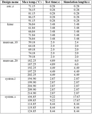
9.22 seconds to 8.44 seconds when the thermal constraint is increased from 109.85°C to 114.85°C forsystem s. Even more reductions are obtained in terms of simulation effort. For example, forsystem s, increasing the thermal constraint from 109.85°C to 114.85°C reduced the simulation effort by half, from nearly 18 seconds to less than 8.5 seconds.

Design name Power-constrained test scheduling_{Test time(s) Max temp.(°C) Test time(s) Sav.(%) Violations Simulation length(s)}Thermal-aware test scheduling (heuristic)

asic z 0.32 70.81 0.28 12.69 0 0.28

kime 3.81 56.51 3.48 8.42 0 3.48

muresan 10 2.4 58.85 2.0 16.66 1 2.4

muresan 20 5.69 181.79 4.89 14.05 1 6.0

system l 3.05 191.74 2.87 5.09 0 2.87

system s 12.12 104.48 9.22 23.88 1 17.67

Table 5. Power constrained test scheduling vs. heuristic thermal-aware test scheduling

Design name Max temp.(°C) Test time(s) Simulation length(s)

asic z 71.15 0.28 0.28

76.15 0.28 0.28

81.15 0.28 0.28

86.15 0.28 0.28

91.15 0.28 0.28

kime 56.84 3.48 3.48

61.84 3.48 3.48

66.84 3.48 3.48

71.84 3.48 3.48

76.84 3.48 3.48

muresan 10 59.18 2.0 2.4

64.18 2.0 2.0

69.18 2.0 2.0

74.18 2.0 2.0

79.18 2.0 2.0

muresan 20 182.25 4.89 6.0

187.25 4.89 6.0

192.25 4.49 4.49

197.25 4.49 4.49

202.25 4.49 4.49

system l 194.90 2.87 2.87

199.90 2.87 2.87

204.90 2.87 2.87

209.90 2.87 2.87

214.90 2.87 2.87

system s 104.85 9.22 17.67

109.85 9.22 17.67

114.85 8.44 8.44

119.85 8.44 8.44

124.85 8.44 8.44

Table 6. Test times for different temperature constraints

Design name Test time increase(%) Simulation effort reduction(%)

asic z 0 0

kime 0 0

muresan 10 0 -20

muresan 20 16.4 75.9

system l 13.4 43.28

system s 0 67.38

Table 7. Comparison between the exact and the heuristic thermal-aware test scheduling algorithms

4. Conclusions

Overheating has been acknowledged as a major problem during the testing of complex system-on-chip (SOC) integrated circuits. In this paper, we have outlined the need for thermal-safe testing and explained that existing power-constrained test scheduling approaches cannot guarantee thermal safety during test. Next, we have proposed a new test scheduling approach that produces short test schedules and guarantees thermal-safety during test at the same time. Two possible algorithms have been developed for the proposed thermal-safe test scheduling approach. The first proposed algorithm, although computationally expensive, provides an optimal solution to the thermal-safe test scheduling problem. The second algorithm uses a fast heuristic based on a low-complexity test session thermal model in order to reduce the required computational effort while producing optimal or near-optimal test schedules. Experimental results show that up to 24% shorter test schedules can be obtained using the proposed approach without increasing the maximum temperature during test application, when compared to power constrained test scheduling approaches. The proposed approach provides an effective solution to the problems arising from chip overheating during test.

5. Acknowledgements

P. Rosinger and B. M. Al-Hashimi acknowledge the Engineering and Physical Sciences Research Council (EP-SRC) for funding this work under grant no. GR/S05557. The work of K. Chakrabarty was supported in part by the US National Science Foundation under grant no. CCR-0204077. The authors wish to acknowledge Erik Larsson from Linkoping University, Sweden for providing the code and designs used for the work presented in reference [7].

References

[1] K. Chakrabarty. Design of system-on-a-chip test access architectures under place-and-route and power constraints. In

Proc. IEEE/ACM Design Automation Conference (DAC), pages 432–437, 2000.

[3] P. Flores, J. Costa, H. Neto, J. Monteiro, and J. Marques-Silva. Assignment and reordering of incompletely specified pattern sequences targeting minimum power dissipation. In12th International Conference on VLSI Design, pages 37–41, 1999.

[4] A. Gibbons.Algorithmic graph theory. Cambridge University Press, 1985.

[5] P. Girard, C. Landrault, S. Pravossoudovitch, and D. Severac. Reducing power consumption during test application by test vector ordering. InProc. International Symposium on Circuits and Systems (ISCAS), pages 296–299, 1998. [6] V. Iyengar and K. Chakrabarty. System-on-a-chip test with precedence relationships, preemption and power constraints.

IEEE Transactions on Computer-Aided Design of Integrated Circuits and Systems, 21:1088–1094, September 2002. [7] E. Larsson, K. Arvidsson, H. Fujiwara, and Z. Peng. Efficient test solutions for core-based designs.IEEE Transactions

on Computer-Aided Design of Integrated Circuits and Systems, 23(5):758–775, May 2004.

[8] S. Lee, S. Song, V. Au, and K. Moran. Constricting/spreading resistance model for electronics packaging. In

ASME/JSME Thermal Engineering Conference, pages 199–206, 1995.

[9] V. Muresan, X. Wang, V. Muresan, and M. Vladutiu. A comparison of classical scheduling approaches in power-constrained block-test scheduling. InProc. IEEE International Test Conference (ITC 2000), pages 882–891, 2000. [10] National Semiconductor. Understanding Integrated Circuit Package Power Capabilities, April 2000.

http://www.national.com/ms/UN/UNDERSTANDING INTERGRATED CIRCUIT PACKAGE POWER CA.pdf. [11] N. Nicolici and B. Al-Hashimi. Power conscious test synthesis and scheduling for BIST RTL data paths. InProc. IEEE

International Test Conference (ITC 2000), pages 662–671, October 2000.

[12] M. Nourani and J. Chin. Power-time trade off in test scheduling for SoCs. InProc. IEEE International Conference on Computer Design(ICCD), pages 548–553, October 2003.

[13] M. Nourani and J. Chin. Test scheduling with power-time tradeoff and hot-spot avoidance using MILP. IEE Proceed-ings - Computers and Digital Techniques, 151(5):341–355, September 2004.

[14] B. Pouya and A. Crouch. Optimization trade-offs for vector volume and test power. InInternational Test Conference (ITC), pages 873–881, 2000.

[15] C. P. Ravikumar, G. Chandra, and A. Verma. Simultaneous module selection and scheduling for power-constrained testing of core based systems. In13th International Conference on VLSI Design, pages 462–467, 2000.

[16] P. Rosinger. Sample designs for validating thermal-aware test solutions. 2005. http://www.ecs.soton.ac.uk/ pmr/thermal test sample designs.zip.

[17] P. Rosinger, B. Al-Hashimi, and N. Nicolici. Scan architecture with mutually exclusive scan segment activation for shift and capture power reduction. IEEE Transactions on Computer Aided Design of Integrated Circuits and Systems, pages 1142–1154, 2004.

[18] J. Saxena, K. M. Butler, and L. Whetsel. An analysis of power reduction techniques in scan testing. InIEEE Interna-tional Test Conference(ITC), pages 670–677, 2001.

[19] C. Shi and R. Kapur. How power aware test improves reliability and yield. In EETimes. September, 15 2004. http://www.eetimes.com/news/design/features/showArticle.jhtml?articleId=47208594&kc=4235.

[20] K. Skadron, M. Stan, W. Huang, S. Velusamy, K. Sankaranarayanan, and D. Tarjan. Temperature-aware microarchitec-ture. InInternational Symposium on Computer Architecture (ISCA), pages 2–13, 2003.

[21] S. Wang and S. K. Gupta. DS-LFSR: A new BIST TPG for low heat dissipation. InProc. IEEE International Test Conference, pages 848–857, 1997.