Using Age and Spatial Flow Structures in the Indirect Estimation of Migration Streams

U

A

S

F

S

I

E

M

S

J

R

,

A

R

A

This paper presents a modeling strategy for describing and estimating interregional migration

flows. The categorical log-linear model is used to demonstrate various approaches to

estimation, including direct and indirect methods. And estimates of known data on

interdivisional migration patterns in the United States during the 1995-2000 period are used to

illustrate the effectiveness of the various log-linear models. The important aspects of the

modeling strategy presented in this paper include parameter interpretation, incorporation of

auxiliary or a priori information, and assessment of the various model predictions. The results

show that capturing the interactions between origins and destinations are very important for

accurate predictions.

Using Age and Spatial Flow Structures in the Indirect

Estimation of Migration Streams

James Raymer

and Andrei Rogers

September 17, 2005

*

Division of Social Statistics, School of Social Sciences, University of Southampton, Southampton, SO17 1BJ, United Kingdom, e-mail: [email protected]

†

ABSTRACT

This paper presents a modeling strategy for describing and estimating

USING AGE AND SPATIAL FLOW STRUCTURES IN THE INDIRECT ESTIMATION OF MIGRATION STREAMS

1. INTRODUCTION

In the absence of adequate migration data for a particular study region, demographers generally have turned to estimates obtained by combining related information (drawn from several sources, time periods, and geographical areas) with models that impose regularities exhibited by past migration patterns in the particular study region or elsewhere. These efforts often seek to produce estimates of a migration variable on the basis of information that may be only indirectly related to its value, or that may be out of date.

Interdivisional migration data for the United States during the 1995-2000 period are used to illustrate the formal method.

Migration estimation techniques are needed to provide the necessary inputs for better understanding population redistribution patterns and to improve current or projected estimates of population totals. At present, only residual methods to obtain net migration totals and, to a lesser extent, model migration schedules to estimate age patterns of migration have been incorporated into books on demographic methods (e.g., Morrison, Bryan and Swanson 2004; Preston, Heuveline and Guillot 2000; Rowland 2003). On the other hand, there exists a vast literature on methods for estimating fertility and mortality. For most countries in the world, migration is a major component of population change. It is therefore somewhat surprising that more attention is not given to methods for analyzing and estimating migration flows. To find models of migration, one generally has to go to texts on quantitative geography and look for gravity or spatial interaction models (e.g., Fotheringham, Brunsdon and Charlton 2000; Plane and Rogerson 1994; Robinson 1998). Much of the background for this paper comes from developments in spatial interaction modeling made by geographers in the late 1970s and early 1980s (Plane 1981, 1982; Snickars and Weibull 1977; Willekens 1980, 1982, 1983).

2. ORIGIN, DESTINATION, AND AGE STRUCTURES OF INTERDIVISIONAL MIGRATION IN THE UNITED STATES

The data used for this study include the observed age-specific interdivisional migration patterns in the United States during the 1985-1990 and 1995-2000 periods obtained from the 1990 and 2000 censuses, respectively. The emphasis, however, is on analyzing and estimating the migration patterns of the latter period. The 1985-1990 migration patterns are applied as a priori information in the direct estimation model set out in Section 3 of this paper. The U.S. migration data obtained from the 1990 and 2000 censuses represent transition or status migration data, that is, place of residence at the time of the census and five-years prior to the census. These can be distinguished from event migration data obtained from population registers (Morrison, Bryan and Swanson 2004; Willekens 1999).

2.1 Describing Age and Spatial Structures with Multiplicative Components Interdivisional migration flows (without age) can be disaggregated into four separate components (Rogers et al. 2002): an overall component representing the level of migration, an origin component representing the relative “pushes” from each region, a

destination component representing the relative “pulls” to each region, and a two-way

origin-destination interaction component representing the physical or social distance between places (not explained by the overall and main effects). This breakdown is multiplicative, such that

ij j i

ij T*O *D *OD

where nij is an observed flow of migration from region i to region j, T is the total number of migrants (i.e., n₊₊), Oi is the proportion of all migrants leaving from region i (i.e.,

), and D +

+ +/n

n_i j is the proportion of all migrants moving to region j (i.e., ). The interaction component OD

+ + + /n

n _j

ij is defined as nij/

(

)

migration to expected migration (for the case of no interaction). This general type of model is termed a multiplicative component model.

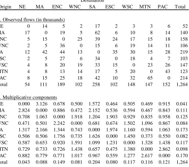
To illustrate the advantages of analyzing migration in terms of multiplicative components, consider the U.S.-born migration flows between the nine Census Bureau-defined divisions during the 1995-2000 time period set out in Panel A of Table 1. Note that non-migrants (i.e., ) are not included in the table. During this period, 14.6 million U.S.-born persons over the age of 5 years made an interdivisional migration. Nearly half of all migrants came from the East North Central, South Atlantic, and Pacific divisions and about a quarter of all migrants went to the South Atlantic division. The largest origin-destination-specific flow was from the Middle Atlantic division to the South Atlantic division.

Table 1. The spatial structure of U.S.-born interdivisional migration (in thousands), 1995-2000

Origin NE MA ENC WNC SA ESC WSC MTN PAC Total

NE 0 167 61 22 298 23 41 59 100 771

MA 245 0 199 54 1,084 74 105 145 191 2,097

ENC 68 161 0 297 674 280 223 273 241 2,217

WNC 25 48 270 0 185 63 205 215 145 1,157

SA 168 437 413 139 0 393 314 215 301 2,380

ESC 18 40 185 47 379 0 159 54 67 947

WSC 37 76 184 188 358 179 0 235 226 1,482

MTN 43 72 154 166 197 53 222 0 472 1,379

PAC 92 151 230 180 397 101 310 766 0 2,227

Total 696 1,150 1,696 1,093 3,573 1,165 1,581 1,962 1,741 14,657

NE 0.000 2.755 0.686 0.388 1.583 0.374 0.494 0.573 1.092 0.053

MA 2.464 0.000 0.820 0.344 2.120 0.445 0.466 0.516 0.765 0.143

ENC 0.647 0.926 0.000 1.794 1.247 1.589 0.934 0.920 0.913 0.151

WNC 0.460 0.523 2.015 0.000 0.658 0.687 1.647 1.390 1.054 0.079

SA 1.486 2.341 1.500 0.786 0.000 2.075 1.225 0.674 1.063 0.162

ESC 0.393 0.532 1.688 0.664 1.641 0.000 1.554 0.425 0.592 0.065

WSC 0.519 0.652 1.071 1.704 0.992 1.516 0.000 1.185 1.281 0.101

MTN 0.653 0.662 0.967 1.612 0.587 0.481 1.495 0.000 2.883 0.094

PAC 0.873 0.862 0.892 1.082 0.732 0.570 1.291 2.570 0.000 0.152

Total 0.047 0.078 0.116 0.075 0.244 0.080 0.108 0.134 0.119 14,657

Destination

B. Multiplicative components A. Observed flows

Note: NE = New England, MA = Middle Atlantic, ENC = East North Central, WNC = West North Central, SA = South Atlantic, ESC = East South Central, WSC = West South Central, MTN = Mountain, and PAC = Pacific.

Atlantic to South Atlantic flow of 1,084 thousand persons disaggregated into the four multiplicative components:

25

n = T*O₂*D₅*OD₂₅

=

( )

= 14,657*0.143*0.244*2.120 = 1,084

The ratio of observed to expected flows captures the relative association or “interaction” between divisions, so the interaction component value of 2.12 indicates a strong association between the Middle Atlantic and South Atlantic regions. Other flows that exhibited high levels of association (over 2.0) were New England-Middle Atlantic, Middle New England, West North Central-East North Central, South Atlantic-Middle Atlantic, South Atlantic-East South Central, Mountain-Pacific, and Pacific-Mountain. In all of these cases, the divisions shared borders with each other.

Next, consider age-specific migration between divisions. The multiplicative component model for this table is specified as:

ijx jx

ix ij

x j i

ijx T*O *D *A *OD *OA *DA *ODA

n = (2)

where the superscript A denotes age and x denotes a five-year age group. The age groups for the U.S. migration data start with 5-9 years and end with 85+ years and are measured at the time the census was taken. In total, there are seventeen age groups. This model is more complicated because there are now three two-way interaction components and one three-way interaction component between the variables origin, destination, and age. However, the interpretations of the parameters remain relatively simple and follow the same format as presented for the two-way table. That is, interaction components represent observed flows or marginal totals to expected ones. For example, the origin-age

interaction component is calculated and represents ratios of observed age profiles of out-migration from each division divided by the overall age profile of migration (as demonstrated below).

) A * O * T /(

The age and spatial structures of U.S.-born interdivisional migration during the 1995-2000 period are described next using the multiplicative components set out above. The analysis follows a hierarchical format starting with the overall level component and ending with the two-way interaction components. The three-way interactions between origin, destination, and age are not analyzed for two reasons. The first is that most of the structure found in the migration patterns is captured by the overall, main, and two-way interaction effects. The second reason is, while there are often patterns found in the three-way interactions, it is tedious to incorporate these into the modeling process and their interpretation is more difficult. Therefore, we just focus on the more simple and powerful aspects of the model represented by the other seven components.

The overall level, origin main effect, destination main effect, and

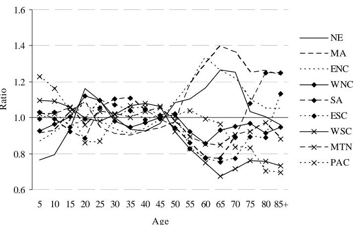
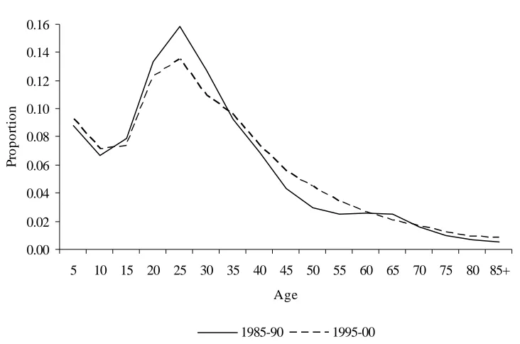
origin-destination interaction components of U.S.-born interdivisional migration have already been presented in Table 1. The values and interpretations remain the same regardless of the number of dimensions in the data, as long as the components are calculated in reference to the total sum. The age-specific shares of all migrants (i.e., the age main effect component) are set out in Figure 4, which shows that the shares of migration were higher for persons in age groups 0-4 to 40-44 years, with a peak occurring in the 25-29 year old age group and the low point occurring for persons in the last age group.

Middle Atlantic, East North Central, and West North Central divisions and less likely to leave the South Atlantic and Pacific divisions. Finally, retirement migrants were more likely to come from the New England, Middle Atlantic, and East North Central divisions.

0.6 0.8 1.0 1.2 1.4 1.6

5 10 15 20 25 30 35 40 45 50 55 60 65 70 75 80 85+

Age

R

a

tio

NE

MA

ENC

WNC

SA

ESC

WSC

MTN

PAC

Figure 1. The origin-age interaction components of U.S.-born interdivisional migration, 1995-2000

0.6 0.8 1.0 1.2 1.4 1.6

5 10 15 20 25 30 35 40 45 50 55 60 65 70 75 80 85+

Age R a tio NE MA ENC WNC SA ESC WSC MTN PAC

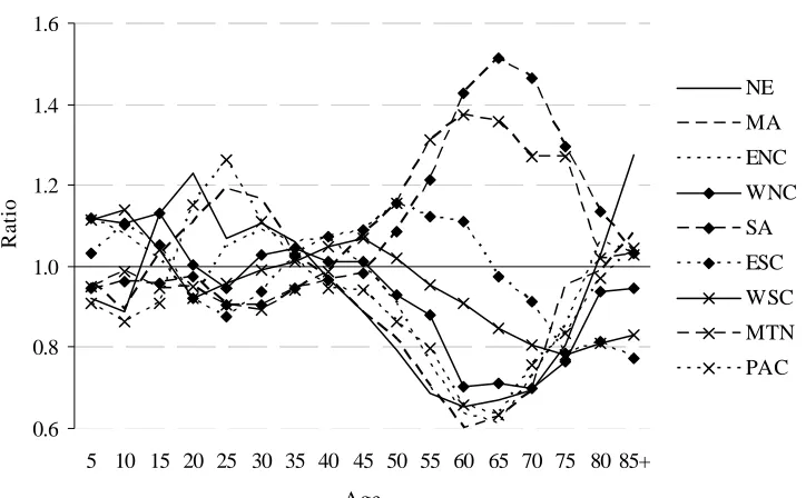
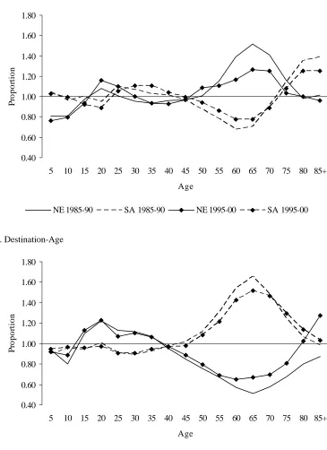
Figure 2. The destination-age interaction components of U.S.-born interdivisional migration, 1995-2000

2.2 The Log-Linear Model for Analyzing Structures in Migration Flow Tables The multiplicative component model set out in Equation 2 used for describing migration age and spatial structures can be expressed as a saturated log-linear model:

ODA ijx DA jx OA ix OD ij A x D j O i ijx) n

ln( =λ+λ +λ +λ +λ +λ +λ +λ (3)

or in multiplicative form:

ODA ijx DA jx OA ix OD ij A x D j O i ijx

where the λ’s or ’s denote the parameters or “effects” of the model. When expressed in this form, migration structures can be modeled using standard statistical techniques for categorical data (see, e.g., Agresti 1996). Also, specific effects can be taken out to identify contributions of the various structures in the data identified by goodness-of-fit measures.

τ

Reduced forms of the models set out in Equations 3 and 4 are considered

unsaturated models. For example, the model that only includes the main effects of origin, destination, and age is specified as

A x D j O i ijx

nˆ =ττ τ τ (5)

This model assumes independence between each of categories of origin, destination, and age and is designated [O][D][A], using the notation set out in Knoke and Burke (1980). A model that includes the interaction between origin and destination plus all of the main effects is designated as [OD] rather than its longer form, [O][D][A][OD]. Similarly the saturated model is expressed as [ODA], which in its longer form would be expressed as [O][D][A][OD][OA][DA][ODA]. The simpler notations are used because these models are hierarchical, that is, for two-way interaction terms, the main effect parameters must be included and for three-way interaction terms all the main effects and two-way interactions must be included.

This model is considered quasi-independent. To do this, an offset is required. This model is specified as:

A x D j O i * ijx ijx n

nˆ = νν ν ν (6)

where the offset, , includes 0’s in the diagonal elements and 1’s in the off-diagonal elements. The ν’s denote the parameters of the log-linear-with-offset model (refer to Rogers, Willekens and Raymer 2003:60-61).

* ij

n

The eight unsaturated models set out in Table 2 all include structural zeros to remove non-migrants from the predictions. We use the likelihood ratio statistic (G2) to compare model fits:

∑

=2 n ln(n /nˆ )

G2 _{ijx ijx ijx} , (7)

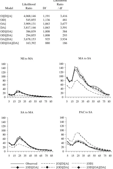
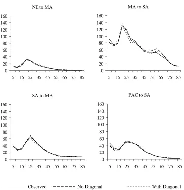
where denotes the predicted age-specific migration flows. The most obvious finding in Table 2 is that the origin-destination interaction term is very important for accurately predicting the age-specific migration flows. Most of the flows do not contain a large retirement peak or major deviations from the overall age profile of migration. However, the fits are slightly improved when the origin-age or destination-age interactions (with the latter doing a better job) are included. This is further demonstrated by the several age- and origin-destination-specific flows illustrated in Figure 3. Of course, to capture retirement peaks found in some of the flows, origin-age or destination-age interactions

Table 2. Unsaturated log-linear model fits: Age-specific U.S.-born interdivisional migration, 1995-2000

Likelihood

Likelihood Ratio

Model Ratio Df / df

[O][D][A] 4,068,146 1,191 3,416

[OD] 545,855 1,136 481

[OA] 3,909,131 1,063 3,677

[DA] 3,817,146 1,063 3,591

[OD][OA] 386,839 1,008 384

[OD][DA] 294,855 1,008 293

[OA][DA] 3,678,153 935 3,934

[OD][OA][DA] 163,392 880 186

NE to MA

0 20 40 60 80 100 120 140 160

5 15 25 35 45 55 65 75 85

MA to SA

0 20 40 60 80 100 120 140 160

5 15 25 35 45 55 65 75 85

SA to MA

0 20 40 60 80 100 120 140 160

5 15 25 35 45 55 65 75 85

PAC to SA

0 20 40 60 80 100 120 140 160

5 15 25 35 45 55 65 75 85

Observed [O][D][A] [OD]

[OD][OA] [OD][DA] [OD][OA][DA]

3. DIRECT ESTIMATION

The 1995-2000 age-specific interdivisional migration patterns are directly

estimated in this section using some of the structures found in the previous census. Much of this work follows recent developments (e.g., see Rogers, Willekens and Raymer 2002, 2003), but the idea of updating tables of migration using iterative proportional fitting algorithms goes back at least to the 1970s (Rogers 1973; Willekens 1977). Efforts to estimate migration flows using historical tables have been shown to be very effective (Isserman et al. 1985; Plane 1982; Rogerson and Plane 1984). Indeed a study by Snickars and Weibull (1977) found that historical data outperformed spatial interaction approaches in such efforts.

To demonstrate the continuity of spatial structures over time, ratios of the 1995-2000 to the 1985-1990 spatial structures (see Equation 1) have been calculated and are set out in Table 3. The ordering of the ratios is the same that was used in Table 1B. Ratios with values close to one indicate continuity in spatial structures over time. For example, consider a comparison over time of the Middle Atlantic to South Atlantic flow

multiplicative components: 90 85 25 00 95 25 n n − −

= ₈₅₉₀

25 90 85 5 90 85 2 90 85 00 95 25 00 95 5 00 95 2 00 95 OD * D * O * T OD * D * O * T − − − − − − − − = 977 . 1 * 263 . 0 * 145 . 0 * 341 , 14 120 . 2 * 244 . 0 * 143 . 0 * 657 , 14

= 1.022*0.988*0.927*1.073

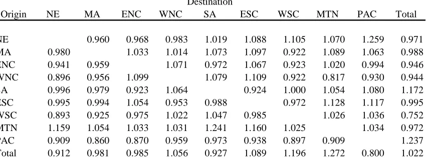
As can be seen with this calculation, there was not much change observed between the 1985-1990 and 1995-2000 periods for the Middle Atlantic to South Atlantic flow. Both the level and the multiplicative components remained relatively close over time. This was true for most, but not all of the multiplicative components. For example, the share of migration from the South Atlantic and Pacific divisions increased by 17 percent and 24 percent, respectively, and decreased by nearly 25 percent in the West South Central division. The proportions of migrants going to the West South Central and Mountain divisions increased substantially, whereas those going to the Pacific division declined. For the origin-destination interaction components, the extremes were those corresponding with the New England to Pacific flow, which increased by 26 percent, and with the West North Central to Mountain flow, which decreased by 18 percent.

Table 3. A comparison of U.S.-born interdivisional migration: Ratio of 1995-2000 spatial structure to 1985-1990 spatial structure

Origin NE MA ENC WNC SA ESC WSC MTN PAC Total

NE 0.960 0.968 0.983 1.019 1.088 1.105 1.070 1.259 0.971

MA 0.980 1.033 1.014 1.073 1.097 0.922 1.089 1.063 0.988

ENC 0.941 0.959 1.071 0.972 1.067 0.923 1.020 0.994 0.946

WNC 0.896 0.956 1.099 1.079 1.109 0.922 0.817 0.930 0.944

SA 0.996 0.979 0.923 1.064 0.924 1.000 1.054 1.080 1.172

ESC 0.995 0.994 1.054 0.953 0.988 0.972 1.128 1.117 0.995

WSC 0.893 0.925 0.975 1.022 1.047 0.985 1.026 1.036 0.752

MTN 1.159 1.054 1.033 1.031 1.241 1.160 1.025 1.034 0.972

PAC 0.909 0.860 0.870 0.959 0.973 0.938 0.897 0.909 1.237

Total 0.912 0.981 0.985 1.056 0.927 1.089 1.196 1.272 0.800 1.022

The age structures also showed consistencies over time. The age main effect components for the 1985-1990 and 1995-2000 periods are set out in Figure 4. The main difference between the two periods is that the labor force peak became slightly wider in the later period. A comparison of New England and South Atlantic’s origin-age and destination-age interaction components for the two migration periods are set out in Figure 5. Here, the most noticeable differences are found in the retirement years where the patterns of the 1995-2000 period are less extreme than in the 1985-1990 period. Overall, the comparisons of the age and spatial structures of migration between the two periods show continuity over time and suggest that a model relying on the 1990 census data used to estimate the 1995-2000 patterns should perform well.

0.00 0.02 0.04 0.06 0.08 0.10 0.12 0.14 0.16

5 10 15 20 25 30 35 40 45 50 55 60 65 70 75 80 85+

Age

P

rop

or

ti

o

n

1985-90 1995-00

A. Origin-Age

0.40 0.60 0.80 1.00 1.20 1.40 1.60 1.80

5 10 15 20 25 30 35 40 45 50 55 60 65 70 75 80 85+

Age

P

rop

or

ti

o

n

NE 1985-90 SA 1985-90 NE 1995-00 SA 1995-00

B. Destination-Age

0.40 0.60 0.80 1.00 1.20 1.40 1.60 1.80

5 10 15 20 25 30 35 40 45 50 55 60 65 70 75 80 85+

Age

P

rop

or

ti

o

n

NE 1985-90 SA 1985-90 NE 1995-00 SA 1995-00

We apply the log-linear-with-offset model (i.e., Equation 6) to directly estimate the 1995-2000 age-specific interdivisional migration flows. The offset in this case is the observed 1985-1990 age-specific interdivisional migration flows. Depending on the available data, the estimation can focus on (1) migrants or (2) both migrants and non-migrants. The first implies that the aggregate numbers of persons in-migrating and out-migrating for each division are known, whereas the second implies that only the

beginning and ending divisional population stocks are known (a more common situation). For the second case, T denotes the overall population size of persons aged 5+ years, Oi denotes the proportion of the population residing in division at the beginning of the interval, Dj denotes the proportion of the population residing in division at the end of the interval, and Ax denotes the proportions of the total population in each age group.

The main concern with modeling migrants and non-migrants is the tendency of non-migrants to dominate the results. During the 1985-1990 and 1995-2000 periods, about 93 percent of the populations were considered non-migrants. For direct estimation modeling, this means that any substantial changes in the non-migrant origin-destination interaction components will have a sizeable impact on the predicted flows of migration. To check this, two offsets were used to estimate the 1995-2000 age-specific

NE to MA 0 20 40 60 80 100 120 140 160

5 15 25 35 45 55 65 75 85

MA to SA

0 20 40 60 80 100 120 140 160

5 15 25 35 45 55 65 75 85

SA to MA

0 20 40 60 80 100 120 140 160

5 15 25 35 45 55 65 75 85

PAC to SA

0 20 40 60 80 100 120 140 160

5 15 25 35 45 55 65 75 85

Observed No Diagonal With Diagonal

Figure 6. A comparison of direct log-linear model predictions: Selected age-specific U.S.-born interdivisional migration flows (in thousands), 1995-2000

data of 0-4 year olds was used to predict age-specific interregional patterns of migration in the United States. The first age group was used because it roughly corresponds with the five-year interval migration question. That is, if a child is living in a different place than his or her place of birth, that child must have migrated at least once during the past five years. The same cannot be said for other age groups. And the reason why a single age group can predict other age groups comes from knowledge of the age regularities found in observed migration patterns.

4.1 Model Migration Schedules

Migration propensities differ greatly according to age. Typically, an age-specific profile of migration shows a downward slope from the early childhood age groups to about age sixteen followed by a rise to a peak in the young adult age groups (usually around age twenty-two), then a gradual tapering off to the oldest age groups. This

“standard” age profile of migration can be fully described using a multiexponential model migration schedule (Rogers and Castro 1981; Rogers and Little 1994).

The most often used model migration schedule is the seven parameter version:

( 1 ) { 2(x 2) exp[ 2(x 2)]

2 x 1 0

ijx a a a

N = + −α + −α −μ − −λ −μ }, i≠ j (8)

where Nijx denotes standardized age profiles of migration from i to j. The a0, a1, and a2 are level parameters, whereas the α₁, α₂, μ₂, and λ₂ parameters are shape parameters.

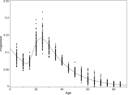
( 0.0429x) {0.0612(x 19.24) exp[ 0.2326(x 19.24)]}

ijx 0.0000 0.1113 0.1885

N = + − + − − − − −

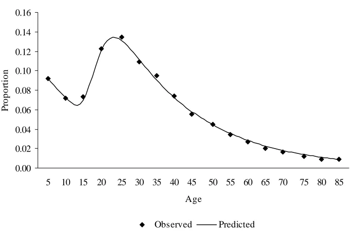
And the predicted curve is set out in Figure 7. Associated with this curve is an R2 of 0.934, which means that nearly all of the 72 age-specific profiles of migration can be explained by a single age profile.

0 20 40 60 80

Age

0 0.05 0.1 0.15 0.2 0.25

Proportion

Figure 7. Model migration schedule fit to standardized age profiles of age-specific U.S.-born interdivisional migration, 1995-2000

( 0.0463x) {0.0501(x 18.37) exp[ 0.2660(x 18.37)]}

x 0.0000 0.1147 0.1603

N₊₊ = + − + − − − − −

and curve set out in Figure 8. All of the parameters were statistically highly significant for both model schedule fits, with the exception of the constant a0 parameter.

0.00 0.02 0.04 0.06 0.08 0.10 0.12 0.14 0.16

5 10 15 20 25 30 35 40 45 50 55 60 65 70 75 80 85

Age

P

rop

or

ti

on

Observed Predicted

Figure 8. Model migration schedule of the age main effect component, 1995-2000

(McDevitt 1996). Congdon (1993) posits that a relational approach for modeling age patterns of migration, similar to Zaba’s (1987), might be more practical. Next, the knowledge that a single age profile of migration can capture most of the age profiles of migration suggests a relational-type model to predict the interdivisional migration patterns.

4.2 A Relational Approach for Modeling Migration Patterns

The log-linear-with-offset model can be thought of as a relational model (Rogers, Willekens and Raymer 2003). In this situation, the offset is the 0-4 year old migration patterns. As can be seen in Table 4, the spatial structure of these lifetime migrants closely resembles that of the period migrants set out in Table 1. A log-linear-with-offset model can be specified which uses the infant migration patterns to predict the aggregate patterns (assuming the marginal totals are known):

D j O i * ij ij n

nˆ = νν ν , (8)

where the offset contains the “migration” patterns of those aged 0-4 years at the time of the census. The predicted aggregate flows from New England and South Atlantic are set out in Figure 9. Two offsets were used: (1) migrants and (2) migrants and non-migrants. While both models appear to predict the observed data well, the migrants-only model did considerably better. The likelihood ratio statistics for the two models were 132,799 and -1,632,755, respectively. The corresponding R

* ij

n

2

Table 4. The spatial structure of U.S.-born interdivisional lifetime migration of 0-4 year olds (in thousands), 2000

Origin NE MA ENC WNC SA ESC WSC MTN PAC Total

A. Observed flows (in thousands)

NE 0 14 5 2 17 2 3 3 6

MA 17 0 19 5 62 6 10 8 14 140

ENC 5 15 0 25 39 24 17 15 18 15

WNC 2 5 36 0 15 6 19 14 11 10

SA 12 42 44 13 0 35 30 15 28 219

ESC 2 5 27 6 34 0 18 4 7 1

WSC 4 8 20 19 33 15 0 23 26 147

MTN 4 8 13 14 17 5 20 0 43 12

PAC 8 15 25 18 42 10 32 65 0 214

Total 54 111 189 102 258 102 148 147 152 1,264

B. Multiplicative components

52

8 6

03

3

NE 0.000 3.126 0.678 0.500 1.572 0.464 0.505 0.469 0.915 0.041

MA 2.824 0.000 0.886 0.472 2.152 0.536 0.594 0.467 0.843 0.111

ENC 0.708 1.063 0.000 1.918 1.204 1.903 0.929 0.835 0.958 0.125

WNC 0.471 0.501 2.242 0.000 0.681 0.674 1.502 1.096 0.867 0.084

SA 1.317 2.166 1.344 0.743 0.000 1.974 1.160 0.594 1.063 0.173

ESC 0.506 0.506 1.756 0.735 1.626 0.000 1.450 0.373 0.550 0.082

WSC 0.587 0.653 0.920 1.591 1.099 1.231 0.000 1.328 1.438 0.117

MTN 0.729 0.733 0.726 1.438 0.657 0.475 1.380 0.000 2.862 0.098

PAC 0.882 0.779 0.771 1.017 0.967 0.559 1.277 2.617 0.000 0.170

Total 0.043 0.088 0.149 0.081 0.204 0.080 0.117 0.116 0.121 1,264

From New England

0 100 200 300 400 500

MA ENC WNC SA ESC WSC MTN PAC

T

hou

sa

n

ds

Destination

observed migrants+non-migrants migrants

From South Atlantic

0 100 200 300 400 500

NE MA ENC WNC ESC WSC MTN PAC

T

h

ou

sa

nd

s

Destination

observed migrants+non-migrants migrants

Figure 9. A comparison of indirect log-linear model predictions: U.S.-born

Two models were used to produce the age-specific predictions set out in Figure 10. The first one is analogous to Equation 6, but with an offset that contains structural zeros (i = j) and the infant migration patterns set out in Table 4. To obtain reasonable projections of the flows that included non-migrants an additional interaction term was required. This model assumes that the aggregate age-specific proportions of migrants and non-migrants are known and is specified as:

AM xz M z A x D j O i * ijxz ijxz n

nˆ = νν ν ν ν ν (9)

NE to MA

0 20 40 60 80 100 120 140 160

5 15 25 35 45 55 65 75 85+

MA to SA

0 20 40 60 80 100 120 140 160

5 15 25 35 45 55 65 75 85+

SA to MA

0 20 40 60 80 100 120 140 160

5 15 25 35 45 55 65 75 85+

PAC to SA

0 20 40 60 80 100 120 140 160

5 15 25 35 45 55 65 75 85+

Observed Structural zeros Diagonal interaction

NE

0.0 0.5 1.0 1.5 2.0 2.5 3.0 3.5

5 15 25 35 45 55 65 75 85+

MA

0.0 0.5 1.0 1.5 2.0 2.5 3.0 3.5

5 15 25 35 45 55 65 75 85+

SA

0.0 0.5 1.0 1.5 2.0 2.5 3.0 3.5

5 15 25 35 45 55 65 75 85+

PAC

0.0 0.5 1.0 1.5 2.0 2.5 3.0 3.5

5 15 25 35 45 55 65 75 85+

Observed Diagonal interaction

5. SUMMARY AND DISCUSSION

The topic of indirect estimation has received wide attention from demographers studying the fertility and mortality patterns of countries with incomplete or inaccurate vital registration data. The Population Division of the United Nations has been an especially significant contributor to the collection, description, and dissemination of the assortment of techniques developed by demographers such as William Brass, Ansley Coale, James Trussell, Donald McNeil, Paul Demeny, and others. In 1983 it published a manual that is still used today. Unfortunately, the indirect estimation of migration was ignored:

A further limitation of the Manual is that it deals mainly with the estimation of fertility and mortality in developing countries. There are other

demographic processes affecting the populations of these countries (migration for example) which are not treated here (United Nations 1983:1).

Our efforts are preliminary in several respects, but the results that we have obtained so far and presented in this paper are encouraging. They suggest a number of questions that need to be addressed in future work. First, we have dealt with numbers, yet the arithmetic of demography generally is carried out with rates or probabilities. Second, we have assumed the availability of historical data from which we might identify and borrow regularities in patterns, applying them to current data. In the absence of such historical data, the methods presented here would need to posit structures, possibly on the basis of “explanatory” models that link the evolution of patterns to a handful of

covariates. For example, we are working on methods that use population age compositions to predict the age compositions of migrants (Little and Rogers 2004; Schmertmann 1992).

BIBLIOGRAPHY

Agresti A. 1996. An introduction to categorical data analysis. New York: Wiley. Congdon P. 1993. Statistical graduation in local demographic analysis and projection.

Journal of the Royal Statistical Society A, 156(2):237-270.

Eldridge HT and Y Kim. 1968. The estimation of intercensal migration from birth-residence statistics. Population Studies Center, University of Pennsylvania, Philadelphia.

Fotheringham AS, C Brunsdon and M Charlton. 2000. Quantitative geography: Perspectives on spatial data analysis. London: Sage.

George MV. 1971. Estimation of interprovincial migration for Canada from place of birth by residence data, 1951-1961. Demography, 8(1):123-139.

Hill K. 1989. Indirect estimation of international migration. Presented at International Population Conference, International Union for the Scientific Study of

Population, New Delhi.

Isserman AM, DA Plane, PA Rogerson and PM Beaumont. 1985. Forecasting interstate migration with limited data: A demographic-economic approach. Journal of the American Statistical Association, 80(390):277-285.

Knoke D and PJ Burke. 1980. Log-linear models. Newbury Park: Sage.

Lin G. 1999. Assessing structural change in U.S. migration patterns: A log-rate modeling approach. Mathematical Population Studies, 7(3):217-237.

Little JS and A Rogers. 2004. What can the age composition of the population tell us about the age composition of migrants? Presented at Colorado Conference on the Estimation of Migration, Estes Park.

McDevitt TM. 1996. Errors associated with using model migration schedules in

subnational projections in a developing country. International Programs Center, Population Division, Bureau of the Census, Washington, DC.

Morrison PA, TM Bryan and DA Swanson. 2004. Internal migration and short-distance mobility. In The methods and materials of demography, Siegel JS and DA Swanson, eds. San Diego: Elsevier Academic Press.

Nair PS. 1985. Estimation of period-specific gross migration flows from limited data: Bi-proportional adjustment approach. Demography, 22(1):133-142.

---. 1982. An information theoretic approach to the estimation of migration flows.

Journal of Regional Science, 22(4):441-456.

Plane DA and PA Rogerson. 1994. The geographical analysis of population: With applications to planning and business. New York: Wiley.

Preston SH, P Heuveline and M Guillot. 2000. Demography: Measuring and modeling population processes. New York: Blackwell.

Robinson GM. 1998. Methods and techniques in human geography. Chichester: Wiley. Rogers A. 1973. Estimating internal migration from incomplete data using model

multiregional life tables. Demography, 10(2):277-287.

Rogers A and LJ Castro. 1981. Model migration schedules. RR-81-30, International Institute for Applied Systems Analysis, Laxenburg, Austria.

Rogers A and L Jordan. 2004. Estimating migration flows from birthplace-specific population stocks of infants. Geographical Analysis, 36(1):38-53.

Rogers A and JS Little. 1994. Parameterizing age patterns of demographic rates with the multiexponential model schedule. Mathematical Population Studies, 4(3):175-194.

Rogers A and J Liu. forthcoming. Estimating directional migration flows from age-specific net migration data. Review of Urban and Regional Development Studies. Rogers A and J Raymer. 1998. The spatial focus of US interstate migration flows.

International Journal of Population Geography, 4:63-80.

---. 2005. Origin dependence, secondary migration, and the indirect estimation of migration flows from population stocks. Journal of Population Research, forthcoming.

Rogers A, J Raymer and KB Newbold. 2003. Reconciling and translating migration data collected over time intervals of differing widths. The Annals of Regional Science, 37(4):581-601.

Rogers A and B von Rabenau. 1971. Estimation of interregional migration streams from place-of-birth-by-residence data. Demography, 8(2):185-194.

Rogers A, FJ Willekens, JS Little and J Raymer. 2002. Describing migration spatial structure. Papers in Regional Science, 81:29-48.

---. 2002. Capturing the age and spatial structures of migration. Environment and Planning A, 34:341-359.

---. 2003. Imposing age and spatial structures on inadequate migration-flow datasets. The Professional Geographer, 55(1):56-69.

Rogers A and RT Wilson. 1996. Representing structural change in U.S. migration patterns. Geographical Analysis, 28(1):1-17.

Rogerson PA and DA Plane. 1984. Modeling temporal change in flow matrices. Papers of the Regional Science Association, 54:147-164.

Rowland DT. 2003. Demographic methods and concepts. Oxford: Oxford University Press.

Schmertmann CP. 1992. Estimation of historical migration rates from a single census: Interregional migration in Brazil 1900-1980. Population Studies, 46(1):103-120. Snickars F and JW Weibull. 1977. A minimum information principle: Theory and

practice. Regional Science and Urban Economics, 7:137-168.

Sweeney SH. 1999. Model-based incomplete data analyses with an application to

occupational mobility and migration accounts. Mathematical Population Studies, 7(3):279-305.

United Nations. 1983. Manual X: Indirect techniques for demographic estimation. New York: Department of International Economic and Social Affairs.

Willekens FJ. 1977. The recovery of detailed migration patterns from aggregate data: An entropy maximizing approach. RM-77-58, International Institute for Applied Systems Analysis, Laxenburg, Austria.

---. 1980. Entropy, multiproportional adjustment and the analysis of contingency tables.

Systemi Urbani, 2/3:171-201.

---. 1982. Multidimensional population analysis with incomplete data. In

Multidimensional mathematical demography, Land K and A Rogers, eds., pp. 43-111. New York: Academic Press.

---. 1983. Log-linear modelling of spatial interaction. Papers of the Regional Science Association, 52:187-205.

---. 1999. Modeling approaches to the indirect estimation of migration flows: From entropy to EM. Mathematical Population Studies, 7(3):239-278.