to EEG data
.
White Rose Research Online URL for this paper:
http://eprints.whiterose.ac.uk/74675/
Monograph:
Zhao, Y., Billings, S.A., Wei, H.L. et al. (1 more author) (2011) Detecting and tracking
time-varying causality with applications to EEG data. Research Report. ACSE Research
Report no. 1027 . Automatic Control and Systems Engineering, University of Sheffield
[email protected] https://eprints.whiterose.ac.uk/ Reuse
Unless indicated otherwise, fulltext items are protected by copyright with all rights reserved. The copyright exception in section 29 of the Copyright, Designs and Patents Act 1988 allows the making of a single copy solely for the purpose of non-commercial research or private study within the limits of fair dealing. The publisher or other rights-holder may allow further reproduction and re-use of this version - refer to the White Rose Research Online record for this item. Where records identify the publisher as the copyright holder, users can verify any specific terms of use on the publisher’s website.
Takedown
If you consider content in White Rose Research Online to be in breach of UK law, please notify us by
Detecting and Tracking Time-varying Causality with Applications
to EEG Data
Y. Zhao, S.A. Billings, H. L. Wei, P.G. Sarrigiannis
Research Report No. 1027
Department of Automatic Control and Systems Engineering
The University of Sheffield
Mappin Street, Sheffield,
S1 3JD, UK
Detecting and Tracking Time-varying
Causality with Applications to EEG Data
Y. Zhao, S. A. Billings, H. L. Wei , P.G. Sarrigiannis
Abstract—This paper introduces a novel method called the ERR-Causality, or Error Reduction Ratio Causality test, that can be used to detect and track causal relation-ships between two signals using a new adaptive forward orthogonal least squares (Adaptive-Forward-OLS) algo-rithm. In comparison to the traditional Granger method, one advantage of the new ERR-Causality test is that it can effectively detect the time-varying direction of linear or nonlinear causality between two signals without fitting a complete model. Another important advantage is that the ERR-Causality test can detect both the direction of interactions and estimate the relative time shift between the two signals. Several numerical examples are provided to illustrate the effectiveness of the new method for causal relationship detection between two signals. An important real application, relating to the analysis of the causality of EEG signals from different cortical sites which can be very useful for understanding brain activity during an epileptic seizure by inspecting the high-resolution time-varying directed information flow, is also discussed.
Index Terms—Causality, Granger, EEG, Time-varying, OLS
I. INTRODUCTION
The detection of hidden interdependencies between the components of complex dynamic systems is an important problem that arises in many research fields. There are several ways to tackle this problem based on using either an explicit generative model that embraces the known nonlinear causal architecture [1], or by simply establishing statistical dependencies between two signals using coherence, phase synchronization, or the Granger causality test. The latter approaches are usually more viable and many methods based on these ideas have been developed recently and applied to the analysis of electrophysiological signals, such as directed coherence and partial directed coherence [2, 3, 4]. However cross correlation methods have two possible drawbacks, one is the requirement for reasonably long data sets, and the other is that correlation may only detect causality of two signals with linear interactions. The minimal required data window size to achieve correct results is important because too wide a window will decrease the temporal resolution of the analysis, which can be fatal if the casual relationship changes rapidly over time, and too narrow
Department of Automatic Control and System Engineering, Univer-sity of Sheffield, UK.
Department of Clinical Neurophysiology, Sheffield Teaching Hospi-tals NHS Foundation Trust, Royal Hallamshire Hospital
a window reduces the statistical reliability.
Signals sampled from the real world are rarely stationary and well behaved, and casual interactions and couplings can typically appear, disappear and reappear, and may become weaker or grow stronger over time. Moreover, most complex systems exhibit nonlinear dynamic be-haviours, which may lead to a possible failure of the cross correlation method. Another established way to solve the causality detection problem is by mutually predicting selected observable measurements based on multivariate autoregressive modelling. Many methods based on this idea have been proposed recently and one of the best established methods is based on the Granger causality test [5]. The key idea of this method is that if a signal X causes a signal Y, the knowledge of the past of both X and Y should improve the prediction of the presence of Y in comparison with the knowledge of the past of Y alone. Many new methods have been developed which extend this idea [6, 7, 8]. However, all these methods require that the system model is fully known or that an unbiased model can be fitted to the data sets before the Granger test can be applied. This is far from straightforward when the underlying system re-lationships are nonlinear and dynamic and the measured observations are noisy because, unless a complete and full model which accounts for any potentially nonlinear noise effects is estimated, the Granger test results will be compromised.
In the present study a new causality test is introduced which overcomes most of the disadvantages of existing methods. The new causality detection method will be referred to as the ERR-Causality or Error Reduction Ratio-Causality test. The key advantage of the new test is that it can be applied to nonlinear dynamic systems, and unlike the Granger based tests, the new method does not depend on the full knowledge or estimation of a complete and unbiased system model. By exploiting an important property of the error reduction ratio (ERR) test that is part of the orthogonal least squares (OLS) algorithm it is shown that the causal flow can be detected even when the model is incomplete. This is a significant advantage when the underlying system is nonlinear and dynamic and the measurements may be noisy, because a complete and full model including a nonlinear noise model, which would normally be required to yield un-biased model estimates is not required and indeed not even the full parameter estimates are used in the test. These advantages mean the test is relatively easy to apply and can be used to track fast transitions between causal effects to detect the direction of linear or nonlinear casual interactions, the strength of these interactions, and to provide an estimate of the time shift between two directional signals. Three numerical examples are
used to illustrate the application of the new test and to show the performance of the method in comparison with other methods. Finally the application of the new method to real high resolution Electroencephalography (EEG) recordings is described and it is shown how the new test can be used to exploit the flow sequence of brain signals which may help to locate the source [9] and understand brain activity during an epileptic seizure.
II. METHODS
Let X = {
x(t)}
and Y = {
y(t)}
be two signals,
t= 1, ..., M, whereM is the data length. The aim of this paper is to measure the casual interaction over time be-tween these two signals. The results can be, for example, at a specific time, the signalX causesY,Y causes X, no interaction or bi-directional interaction between them. For a complex system, the causality is often time-varying and the interaction is often dynamic and nonlinear, which makes the problem more challenging. This section begins with a brief review of the cross correlation and the Granger causality tests associated with this problem, and then presents a new ERR-Causality test.
A. Cross correlation
The cross correlation is the most commonly used method to detect causal interactions between the signals
X andY, and is defined as
φxy(τ) = M
∑
t=τ+1
(
x(t)−x)(y(t+τ)−y)
[M
∑
t=1
(
x(t)−x)2
M
∑
t=1
(
y(t)−y)2
]1/2, (1)
whereτ= 0,±1,±2, ...,±(M−1)andx, ydenote the means ofX, Y respectively. If a well defined peak at lag
τ can be observed in the cross correlation function, this indicates that the signal X lags behind the signal Y if
τ >0, which means thatX causesY from the causality point of view. Or if the signalX lags the signalY when
τ < 0, this means Y causes X. If no well defined peak can be observed, no causality is detected. This method is easy to understand and to implement, and no knowledge of the exact model underlying the interaction is required. However, there are three potential problems. Firstly, correlation may not detect the nonlinear causality between two signals, however most complex real systems are likely to be nonlinear. Secondly, this method can not detect a complicated causality, such as a bi-directional interaction. Thirdly, this method requires relatively long data sets to achieve accurate results, which means the reaction to rapidly changing casuality over time is rela-tively slow.
B. Granger Causality
A well established approach to detect causality in both linear and nonlinear systems is the Granger causality test [5]. To calculate the Granger causality of X to Y, a model has to be pre-established which defines the rela-tionship between the output Y and its past information
Y−
and the past information of the inputX−
, expressed as:
Y =f(Y−
, X−
) (2)
Based on the sampled data the parameters in the model
f(Y−
, X−
) have to be estimated and then the predic-tions of Y based on Y−
alone, and on Y−
and X−
are generated. In both cases, the accuracy of tion may be expressed by the variance of the predic-tion errors for two-dimensional modelling var(Y|Y−)
,
var(Y|Y−, X−)
. The Granger causality of X to Y,
GX→Y, is defined by
GX→Y =ln
var(Y|Y−
)
var(Y|Y−, X−) (3)
The Granger causality of Y toX is defined by
GY→X =ln
var(X|X−
)
var(X|X−, Y−) (4)
The advantages of this method are that if the model structure is chosen appropriately, it can tackle both linear and nonlinear systems. The test is also able to detect a bi-directional causality because the causalities from
Y to X and from X to Y are calculated separately. The required window size of sampled data depends on the dynamical properties of the original signals, and the complexity of the chosen model structure. One possible problem for this method is that if the model structure is not chosen appropriately, for example, the model is missing a significant term or terms, the calculated Granger causality may not be reliable, which will be demonstrated in the second simulation example in sec-tion III-B. Because this test is based on an accurate model then noise models may need to be estimated to ensure the model is unbiased. For nonlinear relationships this will often require a nonlinear noise model. Fitting complete nonlinear dynamics system and noise models is a significant overload for this test. Moreover, this method can only detect the direction of signal flow, but is not able to provide a quantitative insight into the time shift between the two signals.
C. Adaptive-Forward-OLS
model terms to select the most significant model terms which are then included to build models term by term. The significance of each of the selected model terms is measured by an index, called the error reduction ratio (ERR), which indicates how much (in percentages) of the variance change in the system response can be accounted for by including the relevant model terms. Complex nonlinear dynamic models and nonlinear noise models can all be identified using this algorithm.
This section introduces an Adaptive-Forward-OLS algo-rithm which will be used later by modifying the well known forward-regression version of OLS [10]. Consider the linear regression function
y(t) =
N
∑
i=1
pi(t)θi, t= 1, ..., M (5)
where y(t) is the dependent variable or the term to regress upon, pi(t) are regressors, θi are unknown pa-rameters to be estimated and M denotes the number of data points in the data set. Equation (5) can be written as
Y =PΘ (6)
where Y = y(1) .. .
y(M)
, P =
PT(1) .. .
PT(M)
,Θ =
θ(1) .. .
θ(N)
(7) and
PT(t) =(p1(t), ..., pN(t)
)
(8)
MatrixP can be decomposed asP =W ×Awhere
W =
w1(1) ... wN(1) ..
. ... ...
w1(M) ... wN(M)
(9)
is an orthogonal matrix because
WTW =Diag
[ M
∑
t=1
w12(t), ..., M
∑
t=1
w2N(t)
]
(10)
andAis an upper triangular matrix with unity diagonal elements A=
1 a12 a13 · · · a1N
1 a23 · · · a2N
. .. ... ...
1 aN−1N
1 (11)
Therefore, (6) can be rewritten as
Y =W G (12)
where
G=AΘ = [g1, ..., gN]T (13)
The estimation of the original parameters can be com-puted from
ˆ
θN = ˆgN
ˆ
θl= ˆgi−∑Nk=i+1aikθˆk, i=N−1, ...,1
}
(14)
In traditional forward OLS, the cut off value of ERR,
Cof f, to stop the search procedure and determine the number of significant terms can be difficult to select, especially when the level of noise is unknown. Recently, several criteria based on ERR have been developed to monitor and stop the search procedure [13, 14, 15]. This paper introduces an algorithm named the Adaptive-Forward-OLS by utilizing the penalized error-to-signal ratio
P ESRn= 1
(1−λn/M)2
(
1−
n
∑
i=1
[err]i
)
(15)
to monitor the regressor search procedure, where n
denotes the number of selected terms and M denotes the total number of sampled data. The search procedure stops whenP ESRn arrives at a minimum. The effect of the adjustable parameterλon the results is discussed in [16], which suggested thatλshould be chosen between
5 and 10. The value of λ is chosen as 6 for all the examples in this paper based on experience, but other values in this range have also be tested and the results remained correct and unchanged.
The whole procedure of the Adaptive-Forward-OLS al-gorithm can be summarized as follows.
(a) a11= 1,w1(t) =p1(t), andgˆ1=
∑M
t=1w1(t)y(t)
∑M
t=1w 2 1(t)
.
(b) For k = 2, ..., N: aik =
∑M
t=1wi(t)pk(t)
∑M
t=1w 2 i(t)
,i = 1, ..., k−1, akk= 1
wk(t) = pk(t) − ∑k
−1
i=1 aikwi(t), and ˆgk =
∑M
t=1wk(t)y(t)
∑M
t=1w 2 k(t)
. ERR is used as a criterion for model
structure selection, and is defined as
[err]k = ˆg 2 k
∑M
t=1w2k(t)
∑M
t=1y2(t)
(16)
(c) ComputeP ESRk using (15). The search procedure stops whenP ESRk arrives at a minimum.
Noise modelling which will often be required to ensure unbiased models, and is described in [17, 18].
D. A New Granger Causality Test based on the Adaptive-Forward-OLS algorithm
In this section a new modification of the Granger test will be introduced based on the modelling algorithm in
section II-C above. When applying the Granger test, the model is either pre-known, which is often impossible especially for real systems, or the model structure has to be detected and a model estimated as the initial step. It has been shown [19] that the estimator introduced in section II-C combines structure determination, parameter estimation and noise modelling, and when coupled with model validity tests, is particularly powerful in identify-ing parsimonious models for structure-unknown systems. The Adaptive-Forward-OLS algorithm therefore can be a part of the Granger method to improve the identification performance and hence enhance the detection capability of the Granger test.
E. The ERR-Causality Test
The new ERR-Causality test is introduced in this section by tackling the problem another way to detect causality between two signals without the identification of a full or complete model. It is shown that this test has significant advantages compared to existing tests and can be readily applied to linear and nonlinear dynamic systems even with noise corrupted measurements. Consider a bivariate Autoregressive (ARX) model
x(t) =∑px
i=1aix(t−i) +∑pj=1y cjy(t−j) +ex(t)
y(t) =∑qy
i=1biy(t−i) +∑qj=1x djx(t−j) +ey(t) (17) where ex(t), ey(t) denote noise sequences, which can be either white noise or coloured noise. Obviously, if
cj ̸= 0, j ∈ {1, ..., py} and dj ̸= 0, j ∈ {1, ..., qx}, this is a typical bi-directional system, which means X
causes Y, and at the same time Y causes X. Consider initially the causality from X to Y. A NARX (Non-linear Auto-Regressive with eXogenous inputs) model [20] constructed using basic function expansions using a linear-in-the parameters form is introduced to express
Y
y(t) =
N
∑
i=1
θiφi(t) +e(t) (18)
whereθi are unknown parameters,N is the number of the total potential model terms involved, and φi(t) =
φi(ϕ(t)) are model terms generated from a candidate term set, for example,ϕ(t)can be
ϕ(t) ={1, y(t−1), ..., y(t−ny), x(t−1), ..., x(t−nx)}T (19) which includes some simple linear components from the past information ofX andY.
Instead of generating a complete model that has to pass the validity tests, the ERR-Causality test can be summarized in the following.
Initially, construct a candidate term set which typically includes past information of Y, and past information
of X. Apply the Adaptive-Forward-OLS algorithm and computer ERR and PESR values. If the selected signif-icant terms by the Adaptive-Forward-OLS algorithm in section II-C includes any term from the past information of X, this indicates the signal X causes Y during the considered time duration [t−h/2, t+h/2], where h
denotes the sampling window size. The ERR-Causality fromX toY at timet, expressed as FX→Y(t), is then
defined as1. If no component from the past information of X is included in the selected significant terms, this indicates that X has no interaction with Y during [t−h/2, t+h/2], andFX→Y(t)is defined to be0. The
strength of FX→Y(t) can be estimated by the summed
ERR values of all the selected terms from X−
, the maximum strength being1.
The selection of the candidate term set can be much more complicated than (19), and will depend on the pre-known information of the considered system. For example, (20) shows a candidate term set with some non-linear components.
ϕ(t) ={ y(t−1), y(t−2), ..., y(t−ny),
x(t−1), x(t−2), ..., x(t−nx),
y(t−1)x(t−1), ..., y(t−1)x(t−nx),
y2(t−1), y2(t−2), ..., y2(t−n y),
x2(t−1), x2(t−2), ..., x2(t−n x)}T
(20) If any significant term that includes any component from the past information ofXis chosen in the ERR-Causality test, this method, theoretically, is able to observe the causality from X to Y, even though ϕ(t) may not include a complete set of all the correct terms of the system. This advantage is based on the fact that the order of the ERR values or the order of term selection produced by the Adaptive-Forward-OLS algorithm is correct even when a complete model is not estimated. This important result, which is fundamental to the ERR-Causality test, will be proved next.
Consider the model
y(t) =
N
∑
i=1
wi(t)gi+ζ(t), t= 1, ..., M (21)
where the first N terms represent all the correct model terms andζ(t)is a white noise sequence with zero mean. Assume onlyNp terms are selected and the other terms are not considered inϕ(t). Note that noise terms can be included in theN terms in the model (21), which should then reduceζ(t)to be white. Then (21) can be expressed as
y(t) =
Np
∑
i=1
wi(t)gi+ N
∑
j=Np+1
Now (22) can be rewritten as
y(t) =
Np
∑
i=1
wi(t)gi+e(t) (23)
where
e(t) =
N
∑
j=Np+1
wj(t)gj+ζ(t) (24)
represents missing model terms and can be viewed as coloured noise and may not be zero mean. Squaring both sides of (23) and taking the expected value gives
E[y2(t)]= E[∑Np
i=1w2i(t)gi2
]
+
2E[∑Np
i=1wi(t)gie(t)
]
+
E[e2(t)]
(25)
Obviously,
E
[(Np
∑
i=1
wi(t)gi
)2]
=E
[Np
∑
i=1
w2i(t)gi2
]
(26)
because w(i)are orthogonal,w(i)w(j) = 0 (i̸=j). Then (25) can be rewritten as
1
M
M
∑
t=1
y2(t)−
Np ∑ i=1 1 M M ∑ t=1
wi2(t)gi2=α (27)
where
α= 2E
[ Np
∑
i=1
wi(t)gie(t)
]
+E[e2(t)] (28)
Replacing e(t) in (28) by (24)
α= 2E
[
∑Np
i=1wi(t)gi
(
∑N
j=Np+1wj(t)gj+ζ(t)
)]
+E
[ (
∑N
j=Np+1wj(t)gj+ζ(t)
)2]
= 0 + 0 +E
[
∑N
j=Np+1w
2 j(t)gj2
]
+E[ζ2(t)]
= M1 ∑M
t=1
∑N
j=Np+1w
2
j(t)g2j+M1
∑M
t=1ζ2(t) (29)
Substituting α back into (27) and dividing
1 M
∑M
t=1y2(t)to both side produces
1− ∑Np i=1 1 M ∑M
t=1w 2 i(t)g 2 i 1 M ∑M
t=1y
2(t) = 1
M
∑M
t=1
∑N
j=Np+1w 2 j(t)g 2 j+ 1 M ∑M
t=1ζ 2
(t)
1 M
∑M
t=1y 2(t)
(30)
Based on the definition of ERR in (16), finally this yields
1−
Np
∑
i=1
[err]i = N
∑
j=Np+1
[err]j+
σ2 ζ
σ2 y
(31)
whereσζ, σy denote the standard deviation ofζ(t), y(t) respectively. Equation (31) implies that the ERR values for the selected terms can be calculated quite indepen-dently of the un-selected terms of the correct term set. Hence, the proposed ERR-Causality method can always provide a correct order of significant terms without fitting a complete model. In other words, even when not all the significant terms are included in ϕ(t), this method should still detect the causality. Notice also that it is only the ERR values that are used in the test, there is no requirement to fit a complete model or no requirement to even estimate all the model parameters. The ERR-Causality test is therefore a more powerful and robust causality detection method, and moreover, many time consuming calculations can be considerably avoided or reduced because the search procedure is monitored by PESR and no further parameter estimation is required. Notice that the method automatically defaults to select just linear terms if the relationship is linear but can also accommodate complete nonlinear dynamics relationships without full model estimation.
III. SIMULATION STUDIES
This section discusses the efficiency and performance of the proposed new method by comparing results with the cross correlation and the Granger test method. The first example demonstrates the procedure including how to select significant terms and measure the value of ERR-Causality. The second and third examples demonstrate the advantages of the new method and the flexibility of term selection and reaction speed to causality changing over time.
A. Example 1
Consider an ARX model expressed as
y(t) =b1y(t−1)+b2y(t−2)+d1x(t−1)+d2x(t−2)+ζ(t) (32) whereζ(t)is a white noise of zero mean and a standard deviationσ= 0.05. In the first test, the parameters were set as b1 =−0.6, b2 = 0.2, d1 = 0.2, d2 = 0.1, which indicatesY depends on the past information of itself and
X, or from the causality point of view,Y is caused by
X. The model was simulated by setting the signalx(t)as a random sequence uniformly distributed in [−0.5,0.5]
and 1000 data point were collected after the system behaviour had settled down. The initial candidate term setϕ(t)was chosen as
{1, y(t−1), y(t−2), y(t−3), x(t−1), x(t−2), x(t−3)}T
(33) The results of term selection associated with the PESR values from the Adaptive-Forward-OLS algorithm are
TABLE I
THE LIST OF SORTED TERMS ASSOCIATED WITHPESRVALUES FOR THE FIRST TEST OFEXAMPLE1.
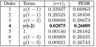
Order Terms [err]i PESR
1 x(t−1) 0.33937 0.66863 2 y(t−1) 0.28525 0.38456 3 x(t−2) 0.09888 0.28673 4 y(t-2) 0.02875 0.26009 5 1 0.00140 0.26182
6 x(t−3) 0.00069 0.26435 7 y(t−3) 0.00021 0.26743
shown in TABLE I. It can be clearly seen that PESR arrives at the minimum 0.26009 when the number of selected terms is 4, which indicates the first 4 selected terms are significant and all the others can be discarded. Note in practice when using the Adaptive-Forward-OLS algorithm, the search procedure will stop after the first5
terms, but the results of all terms are listed in TABLE I to show the trend of PESR in more detail. Because the past information ofX,x(t−1)andx(t−2)are included in the selected terms, the value of ERR-Causality from
X toY,FX→Y, is detected as 1, and the corresponding
strength is0.43825(the sum of ERR values forx(t−1)
and x(t−2)). Notice that the maximum strength is 1
because the ERR values for all terms sum to 1. In the second test, the parameters were set as b1 =
−0.6, b2= 0.2, d1= 0, d2= 0, which indicates there is no interaction betweenX andY. The initial conditions and the candidate term set were exactly the same as those in the first test and the results are shown in TABLE II. It is shown that PESR arrives at the minimum0.38921
TABLE II
THE LIST OF SORTED TERMS ASSOCIATED WITHPESRVALUES FOR THE SECOND TEST OFEXAMPLE1
Order Terms [err]i PESR
1 y(t−1) 0.60121 0.40362 2 y(t-2) 0.01886 0.38921 3 x(t−2) 0.00067 0.39329 4 x(t−1) 0.00031 0.39781 5 x(t−3) 0.00010 0.40264 6 y(t−3) 0.00006 0.40761 7 1 0.00005 0.41268
when the number of selected terms is 2, which indicates only the first 2 terms are significant and all others can be discarded. Because the selected terms contain no past information ofX, based on the definitions in this paper, the value of ERR-Causality from X to Y, FX→Y is detected as 0 with a strength of0.
0 200 400 600 800 1000 -1.5
-1.0 -0.5 0.0 0.5 1.0 1.5
t
x(t)
y(t)
(a)
0 200 400 600 800 1000 0
1
F X->Y F
Y->X
O
r
i
g
i
n
a
l
C
a
u
s
a
l
i
t
y
t
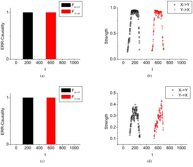
[image:8.612.110.265.121.197.2] [image:8.612.110.263.539.615.2](b)
Fig. 1. (a) The original signalx(t)andy(t)for Example 2. (b) The true causality of the signalX toY and the signalY toX over time, which showsFX→Y = 1during interval100−300andFY→X= 1
during interval500−700.
B. Example 2
This example aims to demonstrate the flexibility of the proposed new method in term selection in comparison with that of the Granger method. A total number of
1000 data points were generated using a time-varying model based on the definition in TABLE III, where
ζy(t), ζx(t)were white noise sequences with zero mean and a standard deviation σ = 0.1, and r(t) denotes a random data sequence uniformly distributed in [−1,1]. To save space, the notationy(t−1)is simplified asy−1
, and so on. Fig. 1.(a) shows the simulated signals ofX
andY, and the true time-varying causality is shown in Fig. 1.(b), both of which and the model clearly indicate: the signalX causes Y at time100−300; the signalY
causesX at time500−700; with no causality at other times.
TABLE III
THE TIME-VARYING MODEL FOREXAMPLE2
t x(t) y(t)
0−100 r(t) r(t)
101−300 r(t) −0.07x−1+ 0.32x−2−x−1x−2+ζy(t)
301−500 r(t) r(t)
501−700 −0.07y−1+ 0.32y−2−y−1y−2+ζ
x(t) r(t)
701−1000 r(t) r(t)
model
y(t) = a(t) +∑3
i=1bi(t)y(t−i) +∑3i=1ci(t)x(t−i)
+∑3
i=1
∑3
j=idij(t)y(t−i)y(t−j)
+∑3
i=1
∑3
j=ifij(t)x(t−i)x(t−j)
+∑3
i=1
∑3
j=ihij(t)x(t−i)y(t−j) +ζy(t) (34) where parametersa, b, c, d, f, h are no longer constants, but functions of time. The window size was chosen as
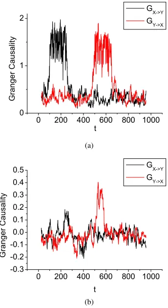
50 and the detected time-varying Granger causality is illustrated in Fig. 2.(a), where an accurate causality can be achieved if an appropriate threshold is used. This is essentially all implementation of the new algorithm described in section II-D.
Now a scenario when some key model terms are missed in the model structure is considered. By removing all the nonlinear terms in (34), the model
y(t) = a(t) +∑3
i=1bi(t)y(t−i) +∑3i=1ci(t)x(t−i)
+ζy(t)
(35) was used and the detected time-varying Granger causal-ity is illustrated by Fig. 2.(b), where the measurabilcausal-ity of causality is significantly decreased and accurate results can not be achieved. This failure arises due to the large contribution of the termx(t−1)x(t−2)in the original model. The absence of this term in the model can dramatically change the signal to noise ratio (SNR) in
Y and results in a very poor prediction ofY even when the past information ofX is considered. This shows the disadvantage of any test based on a knowledge of a full and complete model.
The second test applied the ERR-Causality method.
0 200 400 600 800 1000 0
1 2
G X->Y G
Y->X
G
r
a
n
g
e
r
C
a
u
s
a
l
i
t
y
t
(a)
0 200 400 600 800 1000 -0.3
-0.2 -0.1 0.0 0.1 0.2 0.3 0.4 0.5
G X->Y G
Y->X
G
r
a
n
g
e
r
C
a
u
s
a
l
i
t
y
[image:9.612.333.505.211.526.2]t (b)
Fig. 2. (a) The detected time-varying Granger causality based on the model (34) for Example 2, where the causality is distinctive. (b) The detected time-varying Granger causality based on the model (35) for Example 2, where the causality is not distinctive.
Initially, the candidate terms set was chosen as
{
1,
x(t−1), x(t−2), x(t−3), y(t−1), y(t−2), y(t−3), x2(t−1), x(t−1)x(t−2), x(t−1)x(t−3), x2(t−2),
x(t−2)x(t−3), x2(t−3),
y2(t−1), y(t−1)y(t−2), y(t−1)y(t−3), y2(t−2),
y(t−2)y(t−3), y2(t−3),
x(t−1)y(t−1), x(t−1)y(t−2), x(t−1)y(t−3), x(t−2)y(t−1), x(t−2)y(t−2), x(t−2)y(t−3), x(t−3)y(t−1), x(t−3)y(t−2), x(t−3)y(t−3)}T
(36)
which has28members. The detected time-varying ERR-Causality is illustrated in Fig. 3.(a) which clearly shows the results are consistent with the expected causality. The corresponding strength is shown in Fig. 3.(b), which illustrates the consistently strong strength during interactions. To study the flexibility of the new ERR-Causality test in term selection, the candidate term set was deliberately chosen to be insufficient
{
1, x(t−1), x(t−2), x(t−3), y(t−1)
, y(t−2), y(t−3)}T (37)
where all nonlinear terms have been removed and now only7linear terms were considered. The detected values of the ERR-Causality test, illustrated in Fig. 3.(c), are relatively accurate even though a significant nonlinear term with a large contribution was not considered, and a complete parameter set was not estimated. The corre-sponding strength of the causality is shown in Fig. 3.(d), which illustrates the strength during interactions is not as strong as shown in Fig. 3.(b) due to the absence of the non-linear term, but is still distinctive enough to reflect the original causality. A comparison between Fig. 2.(b) and Fig. 3.(c) shows the robustness of the ERR-Causality test compared to the Granger test. It is well understood that the estimation accuracy for both methods can be improved with an increasing number of trials, but for a real system, multi-trials is often impossible.
Note, the start and end positions ofY causesX andX
causesY in Fig. 3 are not exactly the same as the original model, which is not surprising because the window size determines the reaction speed of causality detection. A selection of small window size means a fast reaction to the change of causality over time, but may lead to insufficient data to achieve an accurate result. Conversely a selection of a large window size can improve the accuracy of causality detection, but may significantly slow down the reaction to the change of causality over time.
C. Example 3
This example aims to explore the application of the proposed method in the estimation of the time shift between two signals, and compares the performance to the cross correlation method using the same window size. Assuming X causes Y at time t, the time shift is approximated by the time lag of the first term from past information of X appearing in the detected significant terms ranked by ERR. For example, if x(t−3) is the first selected term, the time shift ofX causingY at time
tis3 times the sample interval. The contribution of the first term can also be used to approximate the strength of the causality at that time shift.
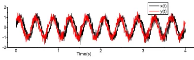
0 1 2 3 4
-2 -1 0 1 2
Time(s)
[image:10.612.328.525.71.132.2]x(t) y(t)
Fig. 4. The generated signalx(t)andy(t)for Example 3.
Consider two signals
x(t) =sin(2πf1t) + 0.2sin(2πf2t) +ζx(t)
y(t) =sin(2πf1t+β) + 0.2sin(2πf2t) +ζy(t) (38) Because the next example involves real EEG data, two common frequencies which appear in real EEG ex-periments were introduced in this simulation. One is the dominant frequency from EEG, which is typically around2−3Hz, and will be denoted byf1; another is
50Hz induced from electrical interference, denoted by
f2. Obviously, y(t) has a fixed phase shift β in front of x(t)at all time. From the causality point of view, Y
causesX at all time with a fixed time shift, which can be expressed τ = 2πβ×f1. Model (38) was simulated by
setting the parameters f1 = 2.5Hz, f2 = 50Hz,∆t =
0.004sec, β= 0.2πandζx(t)andζy(t)are white noise. It can be calculated that the original time shiftτ equals
40ms. Fig. 4 shows the signals X and Y with noise standard deviationσ(
ζx(t))= 0.2 andσ(ζy(t))= 0.2. The candidate terms set for the ERR-Causality test was chosen as
{
1, x(t−∆t), ..., x(t−15∆t), y(t−∆t),
..., y(t−15∆t)}T (39)
The detected time shifts from the ERR-Causality test and the cross correlation method using different window sizes are shown in Fig. 5, where it is expected that the accuracy of estimatedτ for both methods will improve with an increase in window size. Comparison of the results with the same window size for the two methods clearly indicates that the ERR-Causality test requires less samples of data to achieve the same accuracy forτ. This means that the ERR-Causality test has faster reactions to the change of time shift over time than that of the cross correlation method. Several tests suggested that the selection of a window size of 0.5−0.8 times the period of the dominant wave always produces the best performance.
IV. APPLICATION TOEEGDATA
0 200 400 600 800 1000 0
1
F X->Y F
Y->X
E
R
R
-C
a
u
s
a
l
i
t
y
t (a)
0 200 400 600 800 1000 0.0
0.5 1.0
X->Y
Y->X
S
t
r
e
n
g
t
h
t (b)
0 200 400 600 800 1000 0
1
F X->Y F
Y->X
E
R
R
-C
a
u
s
a
l
i
t
y
t (c)
0 200 400 600 800 1000 0.1
0.2 0.3 0.4 0.5
S
t
r
e
n
g
t
h
t
X->Y
Y->X
[image:11.612.114.497.73.404.2](d)
Fig. 3. (a)-(b) The detected time-varying causality with corresponding strength based on the candidate terms set (36) using the ERR-Causality test for Example 2. (c)-(d) The detected time-varying causality with corresponding strength based on the candidate terms set (37) using the ERR-Causality test for Example 2.
correlation and coherence measures [23, 24, 25] or phase synchronisation measures [26, 27]. These methods measure the strength of the interactions between signals, but no insight into the directionality of information flow is produced. The Granger method has also been used to understand the directed interactions between neural assemblies [6], but again no quantitative description has been presented to measure the information flow. In this example, a data set consisting of an epileptic sample of scalp EEGs recorded by the EEG Laboratory of Neurophysiology, Sheffield Teaching Hospitals NHS Foundation Trust, Royal Hallamshire Hospital, were studied to find out the directional flow of signals col-lected from different cortical sites, and to determine the corresponding quantitative measurements of time shift to try to better understand the functional organization of the brain during an epileptic seizure.
In this example, to simplify the problem, only dominant causality is considered at a specific time by comparing
the strength of both causalities.
A. Data acquisition
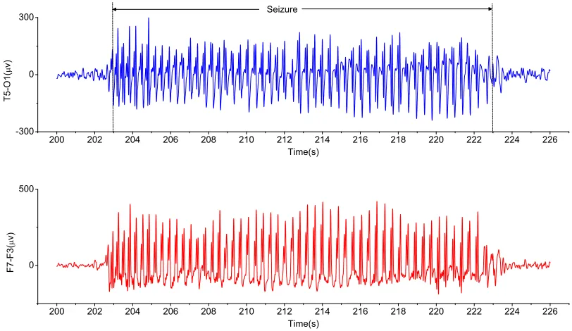
Scalp EEG signals are synchronous discharges from cerebral neurons detected by electrodes attached to the scalp. A NeuroScan Medical System (NeuroSoft Inc., Sterling, VA) with the international 10-20 electrode cou-pling system was used. The samcou-pling rate of the device was 500 Hz. A total of 32 EEG series were recorded in parallel from 32 electrodes located on an epileptic seizure patient’s scalp using the same 32 channel am-plifier system using bipole montage reference channels. This example considered four bipolar montages:F7-F3, T5-O1, F8-F4, T6-O2, which are located in different sites of the brain, as illustrated by Fig. 6. The montage
F7-F3 represents the voltage difference between the channelF7andF3. The purpose of this example is to de-tect the causality associated with the corresponding time shift between the signals from the front and back site
0 1 2 3 4 0 10 20 30 40 50 T i m e s h i f t ( m s ) Time
(a)h= 100
0 1 2 3 4 0 10 20 30 40 50 T i m e s h i f t ( m s ) Time
(b)h= 130
0 1 2 3 4
0 10 20 30 40 50 T i m e s h i f t ( m s ) Time
(c)h= 200
0 1 2 3 4 0 10 20 30 40 50 T i m e s h i f t ( m s ) Time
(d)h= 100
0 1 2 3 4 0 10 20 30 40 50 T i m e s h i f t ( m s ) Time
(e)h= 130
0 1 2 3 4
0 10 20 30 40 50 T i m e s h i f t ( m s ) Time
[image:12.612.94.511.78.322.2](f)h= 200
Fig. 5. (a)-(c): The detected time shift ofY in front ofXusing the cross correlation method with different sizes of windowh; (d)-(f): The detected time shift ofY in frontXusing the ERR-Causality test with different sizes of windowh.
200 202 204 206 208 210 212 214 216 218 220 222 224 226
-300 0 300 T 5 -O 1 ( v ) Time(s) Seizure
200 202 204 206 208 210 212 214 216 218 220 222 224 226
0 500 F 7 -F 3 ( v ) Time(s)
Fig. 7. The recorded EEG signals from the left brain.
of the brain. A comprehensive seizure of a patient was sampled (13000 data points) starts from the 200th sec to the 226th sec. Two experiments were implemented,
[image:12.612.99.505.374.609.2]Fig. 6. Distribution of EEG channels in the brain.
epileptic seizure where regular oscillation starts at the
203rd sec and ends at the 223rd sec. Apply the ERR-Causality test, the candidate term set was chosen as
{
1, x(t−∆t), ..., x(t−20∆t), y(t−∆t),
..., y(t−20∆t)}T (40)
and ∆t = 2ms. The window size was chosen as 300, which will depend on the dominant frequency of the signals as suggested in Example 3. Fig. 8.(a) shows the contribution of the first term from the past information of the other signal detected by the proposed approach, where the black scattering denotes the strength of the signal F7-F3 causing T5-O1, and the red scattering denotes the strength of the signal T5-O1 causing F7-F3. The corresponding values of ERR-Causality test between these two signals are shown in Fig. 8.(b). Inspection of both figures shows that during the time interval 200.5−202 sec, before the epileptic seizure,
F7-F3causingT5-O1dominates the interactions. During the time interval 202 −223 sec, T5-O1 causing F7-F3 dominates the interaction, although F7-F3 causing
T5-O1 appears occasionally with very short duration, especially during 202 −212 sec the strength of T5-O1 causingF7-F3is relatively higher and the causality is more consistent than that during 212 − 223 sec. During the time interval223−226sec, after the seizure, two causalities appear alternatively with relatively small strength. The detected time shift of the signalT5-O1in front ofF7-F3is shown in Fig. 8.(c). It is observed that, during the stable procedure of the epileptic seizure (time intervals 203−223 sec), the detected time shift of the signalT5-O1in front ofF7-F3is very consistent (the av-erage value is about28ms), although a few gaps appear indicating when the opposite causality is detected. From the causality point of view, this observation indicates the signalT5-O1 may cause F7-F3during the seizure with an averaged time shift of about28ms.
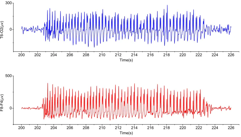
In the second experiment, the montages F8-F4and T6-O2, two signals from the right brain, were sampled after noise removal and the data are shown in Fig. 9. Using the same settings of the parameters, the results produced by the new approach are illustrated by Fig. 10. Fig. 10.(a) shows the contribution of the first term from the past information of the other signal detected by the proposed approach, where the black scattering denotes the strength of the signalF8-F4causingT6-O2, and the red scattering denotes the strength of the signal T6-O2 causing F8-F4. The corresponding values of ERR-Causality test between these two signals are shown in Fig. 10.(b). Inspection of both figures shows that during the time interval 200 − 202 sec, before the epileptic seizure, two causalities appear alternatively with relatively small strength. During the time interval 202−223 sec, T6-O2causingF8-F4completely dominates the interaction with relatively higher strength. During the time interval
223−226 sec, after the seizure, two causalities appear alternatively again with relatively small strength. The detected time shift of the signalT6-O2in front ofF8-F4
is shown in Fig. 10.(c). The observations are very similar as those of the first experiment. During the stable interval of the seizure, the detected time shift of the signalT6-O2
in front ofF8-F4is relatively consistent. Before the start and after the end of the seizure the time shift appears to be chaotic or random. This observation indicates the signalT6-O2 may cause F8-F4during the seizure with an averaged time shift of about 23ms.
Four more epileptic seizures from the same patient have also been studied and the observations of causality are very similar, and the averaged time shifts during the seizure are very close, as shown in TABLE IV, which demonstrates that the time shift of the considered two signals is within the range of25−32ms.
TABLE IV
THE DETECTED AVERAGED TIME SHIFT FOR5SEIZURES FROM THE SAME PATIENT.
Interval τ(T5-O1→F7-F3) τ(T6-O2→F8-F4)
14−40s 27.46ms 25.19ms
202−223s 28.03ms 22.90ms
560−583s 30.04ms 27.90ms
1361−1386s 31.31ms 30.32ms
1674−1694s 31.16ms 29.55ms
All above results produced by the ERR-Causality test indicate the signals from the back brain dominantly causes the signals from the front brain during an epileptic seizure for the studied patient. Moreover, the time shifts of the signal in the left back brain which is in front of the signal in the left front brain were observed to be very
200 202 204 206 208 210 212 214 216 218 220 222 224 226 0.0
0.2 0.4 0.6 0.8 1.0
F7F3->T5O1 T5O1->F7F3
S
t
r
e
n
g
t
h
Time(s)
(a)
200 202 204 206 208 210 212 214 216 218 220 222 224 226
0 1
F F7F3->T 5O1 F
T 5O1->F7F3
E
R
R
-C
a
u
s
a
l
i
t
y
Time(s)
(b)
200 202 204 206 208 210 212 214 216 218 220 222 224 226
0 10 20 30 40 50
T5O1->F7F3
T
i
m
e
s
h
i
f
t
(
m
s
)
Time(s)
(c)
Fig. 8. The results produced by the presented approach for the signalF7-F3andT5-O1. (a) The strength of the ERR-Causality, where the black scattering representsF7-F3causingT5-O1and the red scattering representsT5-O1causingF7-F3; (b) The detected map of the time-varying casuality, where black denotesF7-F3causingT5-O1 and red denotesT5-O1causingF7-F3; (c) The detected time-varying time shift of the signalT5-O1in front ofF7-F3.
close to the time shifts of the signal in the right back brain in front of the signal in the right front brain. For all five epileptic seizures studied in this example, τ(F7-F3
→T5-O1) are slightly different, but consistently longer thanτ(F8-F4 →T6-O2).
The observations extracted from EEG data are very interesting and may provide significant potential in future studies of brain activity during an epileptic seizure.
V. CONCLUSIONS
We have shown that the new ERR-Causality test can detect the time-varying causality of two signals,
[image:14.612.104.508.73.487.2]ERR-200 202 204 206 208 210 212 214 216 218 220 222 224 226 0
300
T
6
-O
2
(
v
)
Time(s)
200 202 204 206 208 210 212 214 216 218 220 222 224 226
0 500
F
8
-F
4
(
v
)
[image:15.612.103.507.80.310.2]Time(s)
Fig. 9. The recorded EEG signals from the right brain.
Causality test to detect the directed interaction between EEG signals has been presented in the last example. By analysing the detected causality map along with the strength and the estimated time shifts, it has been found that the dominant causality is very consistent during epileptic seizure, but the dominant causality before and at the end of seizure are random. Furthermore, the estimated time shifts of the signals from the back brain causing the signals from the front brain are in the range of25−32msfor the studied patient. These observations show that the proposed method could be a very important tool to help understand the functional organization of the brain during an epileptic seizure by providing an insight into directionality of information flow. The results showing the causality between signals from the back brain and the front brain are highly encouraging, and a full map of signal flow will be developed in future publications.
ACKNOWLEDGMENT
The authors gratefully acknowledge that part of this work was financed by Engineering and Physical Sciences Research Council (EPSRC), UK, and by the European Research Council (ERC).
REFERENCES
[1] O. David, S. J. Kiebel, L. M. Harrison, J. Mattout, J. M. Kilner, and K. J. Friston, “Dynamic causal
modeling of evoked responses in eeg and meg,”
NeuroImage, vol. 30, pp. 1255–1272, 2006. [2] L. A. Baccala, K. Sameshima, G. Ballester,
A. C. D. Valle, and C. Timo-laria, “Studying the interaction between brain structures via directed coherence and granger causality,” Applied Signal Processing, vol. 5, pp. 40–48, 1998.
[3] L. A. Baccala and K. Sameshima, “Partial di-rected coherence:a new concept in neural structure determination,” Biological Cybernetics, vol. 84, pp. 463–474, 2001.
[4] H. Ombao and S. V. Bellegem, “Evolutionary coherence of nonstationary signals,” IEEE Trans-actions on Signal Processing, vol. 55, no. 6, pp. 2259–2266, 2008.
[5] C. J. Granger, “Investigating causal relations by econometric models and cross-spectral methods,”
Econometrica, vol. 37, pp. 424–438, 1969. [6] W. Hesse, E.Moller, M. Arnold, and B. Schack,
“The use of time-variant eeg granger causality for inspecting directed interdependencies of neu-ral assemblies,” Journal of Neuroscience Methods, vol. 124, pp. 27–44, 2003.
[7] D. Marinazzo, M. Pellicoro, and S.Stramaglia, “Nonlinear parametric model for granger causal-ity of time series,” Physical Review E, vol. 73, p. 066216, 2006.
[8] J. P. Hamilton, G. Chen, M. E. Thomason, M. E.
200 202 204 206 208 210 212 214 216 218 220 222 224 226 0.0
0.2 0.4 0.6 0.8 1.0
F8F4->T6O2 T6O2->F8F4
S
t
r
e
n
g
t
h
Time(s)
(a)
200 202 204 206 208 210 212 214 216 218 220 222 224 226
0 1
F F8F4->T 6O2 F
T 6O2->F8F4
E
R
R
-C
a
u
s
a
l
i
t
y
Time(s)
(b)
200 202 204 206 208 210 212 214 216 218 220 222 224 226
0 10 20 30 40 50
T6O2->F8F4
T
i
m
e
s
h
i
f
t
(
m
s
)
Time(s)
[image:16.612.104.509.70.488.2](c)
Fig. 10. The results produced by the presented approach for the signalF8-F4and T6-O2. (a) The strength of the ERR-Causality, where the black scattering representsF8-F4causingT6-O2and the red scattering representsT6-O2 causingF8-F4; (b) The detected map of the time-varying casuality, where black denotesF8-F4causingT6-O2and red denotesT6-O2causingF8-F4; (c) The detected time-varying time shift of the signalT6-O2in front ofF8-F4.
Schwartz, and I. H. Gotlib, “Investigating neural primacy in major depressive disorder: multivari-ate granger causality analysis of resting-stmultivari-ate fmri time-series data,” Molecular Psychiatry, vol. 16, no. 7, pp. 763–772, 2011.
[9] J. C. Mosher and R. M. Leahy, “Source localiza-tion using recursively applied and projected (rap) music,” IEEE Transactions on Signal Processing, vol. 47, no. 2, pp. 332–340, 1999.
[10] S. A. Billings, M. Korenberg, and S. Chen, “Iden-tification of non-linear output-affine systems us-ing an orthogonal least squares algorithm,”
In-ternational Journal of Systems Science, vol. 19, pp. 1559–1568, 1988.
[11] M. Korenberg, S. A. Billings, and Y. P. Liu, “Or-thogonal parameter estimation algorithm for non-linear stochastic systems,”International Journal of Control, vol. 48, no. 1, pp. 193–210, 1988. [12] S. Chen, S. A. Billings, and W. Luo, “Orthogonal
least squares methods and their application to non-linear system identification,”International Journal of Control, vol. 50, no. 5, pp. 1873–1896, 1989. [13] Y. Zhao and S. A. Billings, “Neighbourhood
of cellular automata,” IEEE Transactions on sys-tems Man and Cybernetics Part B, vol. 36, no. 2, pp. 473–479, 2006.
[14] S. A. Billings and H. L. Wei, “Sparse model identification using a forward orthogonal regres-sion algorithm aided by mutual information,”IEEE Transactions on Neural Networks, vol. 18, no. 1, pp. 306–310, 2007.
[15] H. L. Wei, S. A. Billings, Y. Zhao, and L. Z. Guo, “Lattice dynamical wavelet neural networks implemented using particle swarm optimization for spatio-temporal system identification,” IEEE Transactions on Neural Networks, vol. 20, no. 1, pp. 181–185, 2009.
[16] S. A. Billings and H. L. Wei, “An adaptive orthog-onal search algorithm for model subset selection and nonlinear system identification,” International Journal of Control, vol. 81, no. 5, pp. 714–724, 2008.
[17] Q. M. Zhu and S. A. Billings, “Fast orthogonal identification of nonlinear stochastic models and ra-dial basis function neural networks,” International Journal of Control, vol. 64, no. 5, pp. 871–886, 1996.
[18] K. Z. Mao and S. A. Billings, “Algorithms for minimal model structure detection in nonlinear dy-namic system identification,”International Journal of Control, vol. 68, no. 2, pp. 311–330, 1997. [19] S. A. Billings, S. Chen, and M. Korenberg,
“Iden-tification of mimo non-linear systems using a forward-regression orthogonal edtimator,” Interna-tional Journal of Control, vol. 49, no. 6, pp. 2157– 2189, 1989.
[20] Y. Li, H. L. Wei, S. A. Billings, and
P. G.Sarrigiannis, “Time-varying model
identification for time-frequency feature extraction from eeg data,” Journal of neuroscience methods, vol. 196, pp. 151–158, 2011.
[21] A. Brovelli, M. Z. Ding, A. Ledberg, Y. H. Chen, R. Nakamura, and S. L. Bressler, “Beta oscillations in a large-scale sensorimotor cortical network: Di-rectional influences revealed by granger causality,”
Proceedings of the National Academy of Sciences of the United States of America, vol. 101, pp. 9849– 9854, 2004.
[22] D. W. Gow, J. A. Segawa, S. P. Ahlfors, and F. H. Lin, “Lexical influences on speech percep-tion: A granger causality analysis of meg and eeg source estimates,” NeuroImage, vol. 43, pp. 614– 623, 2008.
[23] S. L. Bressler and J. A. S. Kelso, “Cortical co-ordination dynamics and congnition,” Trends in Cognitive Sciences, vol. 5, pp. 26–36, 2001.
[24] G. Marrelec, J. Daunizeau, M. Pelegrini-Issac, J. Doyon, and H. Benali, “Conditional correlation as a measure of mediated interactivity in fmri and meg/eeg,”IEEE Transactions on Signal Processing, vol. 53, no. 9, pp. 3503–3516, 2005.
[25] L. Astolfi, F. Cincotti, D. Mattia, F. D. Fallani, G. Vecchiato, S. Salinari, G. Vecchiato, H. Witte, and F. Babiloni, “Time-varying cortical connec-tivity estimation from noninvasive, high-resolution eeg recordings,” Journal Of Psychophysiology, vol. 24, no. 2, pp. 93–90, 2010.
[26] F. Varela, J. P. Lachaux, E. Rodriguez, and J. Mar-tinerie, “The brainweb: phase synchronization and large-scale ingeration,” Nature Reviews Neuro-science, vol. 2, no. 4, pp. 229–239, 2001.
[27] S. Aviyente and A. Y. Mutlu, “A time-frequency-based approach to phase and phase synchrony esti-mation,” IEEE Transactions on Signal Processing, vol. 59, no. 7, pp. 3086–3098, 2011.