White Rose Research Online
[email protected]
Universities of Leeds, Sheffield and York
http://eprints.whiterose.ac.uk/
This is the author’s post-print version of an article published in the
Quarterly
Journal of the Royal Meteorological Society, 138 (666)
White Rose Research Online URL for this paper:
http://eprints.whiterose.ac.uk/id/eprint/76543
Published article:
Ross, AN (2012)
Boundary-layer flow within and above a forest canopy of
variable density.
Quarterly Journal of the Royal Meteorological Society, 138 (666).
1259 - 1272. ISSN 0035-9009
Boundary-layer flow within and above a canopy of variable
density
Andrew N. Ross,
a∗aInstitute for Climate and Atmospheric Science, School of Earth and Environment, University of Leeds
∗Correspondence to: School of Earth and Environment, University of Leeds, LS2 9JT, UK. Email: [email protected]
An analytical model is developed for flow within and above a forest canopy with
a slowly varying canopy density. Results are compared with existing analytical
models for flow over a surface with slowly varying roughness length, and also
with numerical simulations. The results show that the analytical solution is
successful in capturing the behaviour of the flow for small and slowly changing
variations in canopy density. Previous models which only vary the roughness
length and neglect changes in displacement height fail to capture the near
surface flow accurately. Including changes in displacement height as well as
roughness length changes gives results closer to those obtained with the full
canopy model, but even then the flow induced in the canopy leads to significant
differences. The analytical model also highlights the sensitivity of the results to
the parameterization of the vertical component of the turbulent stress tensor,
τ
zz. For shorter wavelength variations in the canopy density the analytical
model breaks down as the more rapid changes in density induce larger flow
perturbations which lead to increased flow into and out of the canopy. This
kind of idealised analytical study provides important insights into the role
of canopy heterogeneities on boundary layer flow. This is important both for
understanding near-surface winds and transport, and also for parameterizing
the effects of surface heterogeneities in large-scale weather and climate models.
Copyright c
0000 Royal Meteorological Society
Key Words: Forest canopy; Inhomogeneous canopy density; Variable surface roughness
Received . . .
1. Introduction
For a number of years there has been significant interest
in flow through forest canopies. To a large extent this has
been driven by a desire to understand transport in and above
forest canopies which is important in understanding and
measuring fluxes of CO2, water vapour, isoprene and other
species which are either emitted or absorbed by vegetation.
Such canopy dynamics are also important in understanding
the effects of surface conditions on low level wind
fields and pressure fields, and in determining appropriate
parameterizations of these in large-scale weather and
climate models. A large amount of this work has focused
on homogeneous canopies on flat terrain, however more
recently there has been a shift to understanding
non-homogeneous canopies and terrain. Lee (2000) gives an
overview of some of the earlier work on non-homogeneous
canopies. More recently interest has primarily been in the
effects of terrain (e.g. Finnigan and Belcher 2004; Ross
and Vosper 2005) and of sharp forest edges (e.g. Irvine
et al.1997; Morseet al. 2002; Yanget al. 2006; Dupont and Brunet 2008, 2009; Dupontet al.2008; Romniger and Nepf 2011). In particular Belcheret al.(2003) produced an analytical model for flow across a canopy edge using similar
methods to those discussed here. In an appendix Coceal
and Belcher (2004) considered the related problem of the
adjustment of a perturbed canopy flow to its equilibrium
values. Rather less attention has been paid to studying
the less dramatic, but potentially still important, effects of
slowly varying changes in canopy properties, and this will
be the focus of the present paper.
Previous studies of slowly varying surface properties
tend to use a roughness length parameterization of the
vegetative canopy rather than an explicit canopy model.
Belcheret al.(1990) developed an analytical model for such roughness length changes. Using a Fourier decomposition
they studied both sinusoidally varying and step changes in
roughness. Numerical studies of slowly varying roughness
length include the large-eddy simulations of Hobsonet al.
(1999). Notably both these studies consider only a change
in the roughness length and neglect the effect of any
displacement height changes, although (as Hobson et al.
1999, point out) the latter are likely to be important in the
real world.
Using ideas from the analytical models of Belcheret al.
(1990) and Finnigan and Belcher (2004) (henceforth BXH
and FB respectively) this paper will develop an analytical
solution for flow within and above a canopy of variable
density. The analytical solution will be compared with
existing solutions for an equivalent rough surface and with
numerical simulations.
2. Theoretical model
Consider the space and time averaged momentum equation
for an incompressible fluid (see e.g. Finnigan 2000)
∂Ui
∂t +Uj
∂Ui
∂xj
=−∂p
∂xi
+∂τij
∂xj
−ca|U|Ui. (1)
where Ui are the velocity components, p is the pressure
field, τij are the stress tensor components. The last term
represents the drag due to the canopy wherec is the drag
coefficient andais the canopy density. Outside the canopy
this term is zero.
Here we assume a forest canopy with a mean canopy
densitya0 and sinusoidal variations about this mean. The
canopy depth, h, and the drag coefficient, c, are kept
constant. The variations have wavelength 4L (by analogy
with the definition ofLin FB), so the wavenumber is given
byk=π/(2L). The perturbed canopy density is given by
a=a0(1 +ηeikx) (2)
where the parameter η determines the magnitude of the
variations in canopy density and is assumed small.
Assuming a mixing-length model with constant mixing
canopy densitya0) can be derived as (see e.g. FB)
UB =
Uheβz/l0 z <0
u∗ κ ln
z+d0
z0
z >= 0
(3)
where l0= 2β3Lc is the canopy mixing length, Lc=
1/(ca0)is the canopy adjustment length (see Coceal and
Belcher 2004) andβ is an empirical constant. The velocity
scale Uh is the velocity at canopy top, u∗ is the friction
velocity at canopy top,z0 is the canopy roughness length,
d0is the canopy displacement height andκis von Karman’s
constant. The vertical coordinate,z, is defined soz= 0is
the canopy top. Matching solutions at canopy top (see e.g.
FB) gives
β=u∗/Uh, Uh=
u∗
κ ln
d0
z0
,
d0=l0/κ, z0=
l0
κe
−κ/β. (4)
Physical we imagine that increasing (decreasing) the
canopy density from its mean value will increase (decrease)
the drag and decelerate (accelerate) the horizontal flow.
This in turn will lead to convergence (divergence) in the
horizontal flow, and hence through continuity will generate
a positive (negative) vertical velocity in the canopy. It is this
process, and the impact of this induced motion on the larger
scale flow, that we wish to investigate.
As in BXH, solutions within and above a canopy of
variable density can be written as
u=UB(z) + ∆˜u(x, z), w= ∆ ˜w(x, z),
p=PB+ ∆˜p(x, z), τ =τB+ ∆˜τ(x, z),
τzz=τzzB+ ∆˜τzz(x, z), (5)
for the streamwise velocity, vertical velocity, kinematic
pressure, kinematic turbulent shear stress andzcomponent
normal stress respectively. The subscript B denotes
background solutions and ∆ a perturbation about that
background state. Again following BXH,U0 (the velocity
scale in the outer region) is a sensible scaling for all
velocities, except for the shear stress term which is scaled
on ρu2
∗. The scaling arguments given in BXH for the
perturbations are followed here, but with the forcing
parameter, η, which controls the variations in canopy
density replacing the parameter M which controls the
variations in surface roughness in BXH. This leads to
UB=U0U, ∆u=U0
η
κu,˜ ∆w=U0
η
κw,˜
∆p=ρU02η
κp,˜ ∆τ=ρu
2
∗
η
κτ ,˜ ∆τxx=ρu
2
∗
η
κτ˜xx,
∆τzz=ρu2∗
η
κ˜τzz (6)
where=u∗/U0 is the small parameter in the expansion
of the solution away from the canopy. For small variations
in canopy density (η1) the perturbations are small
enough that the equations of motion can be linearized
about the basic state. The horizontal and vertical momentum
equations and the continuity equation then become (to
O(η))
U∂u˜
∂x+ ˜w
∂U
∂z =−
∂p˜
∂x+
2
∂˜τxx
∂x +
∂τ˜
∂z
−(1−H(z))
2Uu˜
Lc
+κU
2eikx
Lc
(7)
U∂w˜
∂x =−
∂p˜
∂z+
2
∂τ˜
∂x+
∂τ˜zz
∂z
−
(1−H(z))Uw˜
Lc
(8)
0 = ∂u˜
∂x+
∂w˜
∂z (9)
where H is the Heaviside function defined by H(z) =
0, z <0andH(z) = 1, z >0.
The upper boundary conditions are that the perturbations
all decay far above the canopy so
˜
u,w,˜ p,˜ τ˜→0asz/L→ ∞. (10)
At the top of the canopy the velocity and turbulent stress are
continuous. The mixing length is also assumed continuous,
is continuous at canopy top. At the lower boundary at
the bottom of the canopy a free-slip boundary condition
is used so w˜= 0 at z=−h. It is also assumed that the
canopy is deep enough that all the momentum is absorbed
by the canopy so UB→0 and τ→0 as z→ −h, i.e.
exp(−βh/l0)1.
To develop the solution consider a single Fourier mode
with wavelengthksoX˜ =Xeikxfor any quantityX.
For the shear stress term, the mixing length model gives
τ=lm2
∂U ∂z
2
(11)
toO(η2). The mixing length,l
mis given by
lm=
l z <0
κ(z+d) z >= 0.
(12)
Assuming that the local turbulence is always in equilibrium
with the change in canopy density then
l=l0/(1 +ηeikx) =l0(1−ηeikx+O(η2)) (13)
and
d=d0/(1 +ηeikx) =d0(1−ηeikx+O(η2)). (14)
The shear stress termτis then linearized as
τ=
2κ−1eβz/l0 d
0∂u∂z −eβz/l0
z <0
2κ−1
(z+d0)∂u∂z −z+d0d0
z >= 0.
(15)
Following Belcheret al. (1993) and BXH the perturba-tions inτxxandτzz are modelled asτxx=α1τ andτzz=
α3τ, where the constantsα1= 6.3andα3= 1.7are taken
from BXH and were originally derived from observations in
the atmospheric boundary layer. These are not important at
leading order, but are required for the higher order terms in
the solution.
So far this is very similar to the analysis of FB for flow
over a hill (apart from the additional term in Eq. 7 due
to the variations in canopy density) and to the analysis of
BXH for flow over a surface of variable roughness (with the
addition of the canopy). The difference from the analysis
of FB is that rather than being caused by the vertical
velocities generated as the air flows over the hill, in this case
the pressure field is generated by the (generally smaller)
vertical velocities due to the horizontal canopy flow being
slowed down or accelerated as the canopy drag increases or
decreases.
2.1. Flow within the canopy
2.1.1. Upper canopy solution
As in FB, the pressure within the inner layer and in the
canopy is, to leading order, constant with height so p=
p0(x). This follows from analysis of the vertical momentum
equation, Eq. (8), and the fact that the canopy depth and
inner layer depth are both small compared to the horizontal
lengthscale, L, of the canopy variations. Comparing the
advection and drag terms in the canopy gives
UB∂u/∂x
2UBu/Lc
∼ Uhku
2Uhu/Lc
∼kLc
2 1 (16)
which shows that advection is small in the canopy compared
to the drag term provided the canopy adjustment lengthscale
Lc is small compared to the lengthscale over which the
canopy density varies. The pressure field is a response to
the induced vertical velocity in the flow rather than a leading
order forcing, and so the pressure gradient term might also
be expected to be small. In the upper canopy this may
be true. While the velocity and shear stress perturbations
decay deep within the canopy, the pressure gradient remains
constant and so, provided the canopy is sufficiently deep,
the pressure gradient must become important at some point.
For this reason the pressure gradient is retained.
Therefore, to leading order, the perturbations in the shear
and, on substituting the expression forτ, Eq. (7) becomes
iβkLcp0e−Z =u00+u0−2u−3
κ
βe
Z (17)
where the vertical coordinate is transformed toZ =βz/l0
and a prime denotes differentiation with respect toZ. The
general solution to this differential equation is
u= κ
βZe
Z−1
2ikLcp0e
−Z+AeZ+Be−2Z (18)
where the last 2 terms are the solutions of the homogeneous
equation and A and B are complex constants to be
determined from the boundary conditions at the top and
bottom of the canopy. Using Eqs. 15 and 18 the shear stress
perturbation is
τ= 2β−1
κ
βZe
2Z+1
2ikLcp0+Ae
2Z−2Be−Z
.
(19)
Physically the shear stress cannot grow exponentially deep
in the canopy and soB= 0. The same assumption is made
in FB. Substituting Eq. (18) into the continuity equation,
Eq. (9), and integrating (using the kinematic boundary
condition w= 0 at z=−h) gives the canopy vertical
velocity as
w=−2β2ikLc
κ
β(Z−1)e
Z+ (1 +βh/l
0)e−βh/l0+
1
2ikLcp0(e
−Z−eβh/l0) +A(eZ−e−βh/l0)
. (20)
As hypothesised, the pressure gradient term increases
exponentially in the canopy in the expression foruwhile
the other terms decay exponentially and so it will always
become important in a sufficiently deep canopy.
Note that the term involving p0 in u increases
exponentially with depth in the canopy, while the
background flow decays exponentially, and so for a
sufficiently deep canopy the linearization assumption that
∆uUB will fail. Unlike the problem of flow over a
forested hill studied by FB, the pressure here is not a
leading order driver of the flow, but a response to the flow
caused by variations in canopy density, and therefore is
much smaller. One consequence of this is that the canopy
needs to be much deeper before the non-linearity becomes
important. Comparing the term in u which contains the
pressure gradient and the background flow gives
∆u
UB
∼η β
2κkLcp0exp(−2Z) (21)
and so the condition for the linearization to be valid
throughout the canopy is that
β
2κηkLcp0exp(2βh/l0)1. (22)
This condition is not automatically satisfied. Althoughη,
kLcandp0are all small, the exponential term is large (since
exp(−βh/l0)1) and so for a sufficiently deep canopy it
will dominate.
2.1.2. Deep canopy solution
If the canopy is sufficiently deep that the canopy solution
becomes non-linear then Eqs. (18) and (19) are still valid in
the upper canopy. Deep in the canopy the solution becomes
non-linear because the linearization of the drag term fails. In
this deep canopy limit the stress perturbation, τ, becomes
independent of z and so, as in the solution of FB, the
dominant balance is now between the unbalanced part of
the drag term and the pressure gradient so
−dp0
dx =
U|U|
Lc −
U2
B
Lc
(23)
which is an algebraic equation with solution
U =|UB2 −Lcdp0/dx|1/2sgn UB2 −Lcdp0/dx
(24)
where U is the full (dimensional) horizontal velocity
U =UB+ ∆˜u. As acknowledged by FB this equation is
heuristic, however the assumptions made in deriving it are
simulations (e.g. Ross and Vosper 2005). Unlike the
solution of FB over a hill, thep0 in this expression is the
second order pressure induced by the canopy flow rather
than the leading order pressure perturbation generated by
the inviscid flow over the hill. This deep canopy solution
can be approximated as
U =UB−
1 2
Lcdp0/dx
Uh
exp(−Z) (25)
towards the upper part of the canopy. This form matches
with the upper canopy solution Eq. (18) in the limit
Z→ −∞ in the upper canopy solution. One important
consequence of this deep canopy solution is that flow may
become reversed (U <0) deep in the canopy if the pressure
gradient is large enough, or the canopy is deep enough (i.e.
UB is small enough), whereas the linear solution always
remains positive since the u perturbations must remain
smaller than the background velocityUB.
In the same way as described in FB, a uniformly
valid solution throughout the canopy may be derived by
combining the deep canopy solution with the parts of the
upper canopy solution not involving the pressure term to
give
U =|UB2 −Lcdp0/dx|1/2sgn UB2 −Lcdp0/dx
+
U0
η
κ(
κ
βZe
Z+AeZ) exp(ikx) (26)
in dimensional form. This form agrees asymptotically with
both the upper and lower canopy solutions and provides a
convenient expression which may be applied throughout the
canopy.
In order to calculate the pressure field in the following
sections it is necessary to obtain the canopy-top vertical
velocity field. This can be done using the uniformly
valid canopy solution for U given in Eq. (26), either
by integrating the continuity equation or by calculating
the streamfunction of the flow. In order to do this it is
convenient to splitUinto two parts - the linear upper canopy
part and the non-linear deep canopy part, as done in FB.
This gives
Uu=U0
η κ
κ
βZe
Z+AeZ
exp(ikx) (27)
Ud=|UB2 −Lcdp0/dx|1/2sgn UB2 −Lcdp0/dx
. (28)
The linear part coming from the upper canopy solution is
easily integrated to give a vertical velocity
wu=−U0
η
κ2β
2ikL
cexp(ikx)
κ
β(Z−1)e
Z+
κ β
1 + βh
l0
e−βh/l0+A
eZ−e−βh/l0
!
. (29)
The non-linear, deep-canopy, part has to be integrated by
dividing the canopy up into different regions depending
on the sign of the terms. This non-linear part is however
identical in form to the non-linear component of the canopy
flow in FB. The only differences are in the source and
magnitude of the pressure fieldp0. In particularly over a
variable density canopy it is not known a priori where the
pressure gradient will be zero, or where the term UB2 − Lcdp0/dx will be zero. The solution for wd in this case
is therefore the same as in FB, but with a phase shift
depending on the phase of p0. For completeness these
solutions are given in Appendix A.
2.2. Flow above the canopy
The flow above the canopy is divided into 2 regions, the
inner region where the Reynolds stresses are important and
the outer region where the flow is essentially inviscid. Hunt
et al.(1988) estimate the height of the inner region,hi, as
the solution to the implicit equation
khilog(hi/z0) = 2κ2. (30)
The outer region is further divided into two layers, the
middle layer where the curvature of the mean velocity
which cause it are negligible) and an outer layer where the
flow is potential flow. For a logarithmic wind profile Hunt
et al.(1988) give the height of the middle layer,hm, as the
solution to the implicit equation
hmlog1/2(hm/z0) =L. (31)
In the solution of BXH for flow over a surface of variable
roughness the inner region is divided in two layers. The
shear stress layer (SSL) where Reynolds stress terms are
important makes up most of the inner region. Near the
surface is the thin inner surface layer (ISL) over which the
SSL solution is matched to the no-slip boundary condition
at the surface. The unknown coefficients in the solutions
are determined by asymptotically matching the solutions
between the different layers.
The solution method above the canopy is essentially the
same as that of BXH with the important difference that the
SSL solution is directly matched to the canopy solution at
the canopy top, without the requirement for the ISL. The
same procedure is adopted in FB for flow over a
canopy-covered hill. While the solution procedure is the same as
BXH the matching coefficients take different (complex)
values due to the different matching procedure at the bottom
of the SSL.
The solutions for flow above the canopy are given below.
Details on the derivation can be found in BXH. Note
that some of the notation has been changed slightly for
consistency with that used here.
2.2.1. Shear stress layer
In the shear stress layer above the canopy then (following
BXH) the flow variables are scaled as
u= ˆu, w= ˆw, τ= 2
U(hi)
ˆ
τ , p=−U(hi)ˆp (32)
where hi is the inner layer height. The scaled vertical
coordinate in the SSL is ζ= (z+d)/hi. On substituting
these scaled variables the linearized equations become
(1 +δlnζ)iuˆ+ wˆ
2κ2ζ =ip+
∂ ∂ζ
ζ∂uˆ
∂ζ −
ζ0
ζ
−2δiκ2α1
ζ∂uˆ
∂ζ −
ζ0
ζ
2κ2δ(1 +δlnζ)iwˆ= ∂pˆ
∂ζ + 4κ
4
iδ2
ζ∂uˆ
∂ζ −
ζ0
ζ
−2δκ2α3
∂ ∂ζ
ζ∂uˆ
∂ζ −
ζ0
ζ
ˆ
w=−2iκ2δ
Z ζ
ζ0 ˆ
u(ζ0)dζ0+ ˆwc
ˆ
τ= 1
δ
ζ∂u
∂ζ −
ζ0
ζ
(33)
where ζ0=d0/hi and δ= log−1(hi/z0) is the small
parameter in this region. The canopy top vertical velocity is
given bywˆc. Solutions for the flow variables are expanded
in powers ofδso, for example,uˆ=u(0)+δu(1)+O(δ2).
In order to match the canopy solution to this SSL
expansion it is useful to note thatkLc, which appears in
the canopy solutions, can be written askLc=δ2κ2Lc/hi.
This means that wˆc is O(δ) and so w(0) = 0 from the
integrated continuity equation. Since the pressure field is
induced in response to the vertical velocity at canopy top
then again the leading order pressure field is zero,p(0)= 0. Using these leading order terms the horizontal momentum
equation reduces to
∂ ∂ζ
ζ∂u
(0)
∂ζ
−iu(0)=−ζ0
ζ2. (34)
In order for u(0) to remain bounded as ζ→ ∞ the homogeneous solution of this equation must be of the form
A0K0[2(iζ)1/2] where A0 is the constant of integration
(a matching coefficient to be determined by matching
the solution to the layers above and below) and K0
is the modified Bessel function of zeroth order (as in
BXH). A solution to the inhomogeneous equation can be
found by transforming Eq. (34) using the substitutionss=
2e3iπ/4ζ1/2andu= 16iζ
0vto give the Lommel differential
equation
v00+1
sv
which has a solutionS−3,0(Olveret al.2010) whereS−3,0
is a Lommel function. Note that this form of the equation
could be used to write the general solution in terms of Bessel
functions rather than modified Bessel functions, but for
consistency with previous work, modified Bessel functions
are used. The solution foru(0)is then
u(0) =A0K0(2eiπ/4ζ1/2) + 16iζ0S−3,0(2e3iπ/4ζ1/2).
(36)
AtO(δ)the continuity equation gives
w(1)=−2κ2
Z ζ
iu(0)(ζ0)dζ0=−2κ2
ζ∂u (0) ∂ζ − ζ0 ζ ζ ζ0
=w(1)c −2κ2
"
A0
ζ∂K0
∂ζ −ζ0K
0
00
+ 16iζ0
ζ∂S−3,0
∂ζ −ζ0S
0
00
+ (1−ζ0/ζ)
#
(37)
where
K000 = ∂K0[2(iζ)
1/2]
∂ζ
ζ=ζ0≡d0/hi
, (38)
S000 =∂S−3,0[2e
3iπ/4ζ1/2]
∂ζ
ζ=ζ0≡d0/hi
(39)
andw(1)c is theO(δ)canopy top vertical velocity.
The vertical momentum equation atO(δ)is
∂p(1)
∂ζ =−2κ
2∂τ33
∂ζ = 2κ
2 α3 ∂ ∂ζ ζ∂u (0) ∂ζ − ζ0 ζ . (40)
Integrating and matching with the leading order pressure
perturbation σ(1)(k,0) at canopy top (z= 0, ζ=d/h
i=
ζ0) gives
p(1) =σ(1)+ 2κ2α3
"
A0 ζ
∂K0
∂ζ −ζ0K
0
00
!
+ 16iζ0
ζ∂S−3,0
∂ζ −ζ0S
0
00
+ 1−ζ0
ζ
#
. (41)
The pressure is small (i.e.p0=O(δ)) and therefore the
p0 term is not significant in the expression for u in the
upper canopy. This means that to leading order the matching
coefficientsAandA0can be found without requiring a full
solution in the middle and outer layers. Matchinguandτat
canopy top gives a pair of linear simultaneous equations for
AandA0which can be solved giving
A0=
1−16iζ0
ζ0S000 −
β κS00
ζ0K000 −
β κK00
, (42)
A= K00+ 16iζ
2
0(S00K000 −K00S000 )
ζ0K000 −
β κK00
. (43)
In order to match with the middle layer solution the
expressions forwandpmust be evaluated in the limitζ→
∞. Noting thatK0,ζ∂K0/∂ζ,S−3,0andζ∂S−3,0/∂ζ→0
in this limit we obtain
w∼
n
δ(2κ2(A0ζ0K000 + 16iζ
2
0S000 −1) +w (1)
c ) +O(δ
3)o
p∼ −U(hi)
n
δ(σ(1)−2α3κ2(A0ζ0K000 + 16iζ
2
0S000 −1))
+O(δ3)
o
. (44)
2.2.2. Middle layer
In the middle layer solution the Reynolds stress terms
are negligible at leading order and the effect of
the background velocity gradient dominates over the
streamwise acceleration so the equations of motion reduce
to the single equation
∂2w
∂z2 −
U00
U w= 0 (45)
forw. The general solution of this (see BXH) is
w(0)=B0U+C0U
Z zˆ dzˆ0
U2(ˆz0h
m)
(46)
where zˆ=z/hm and hm is the middle layer height
Substituting this expression for w(0) into the continuity
equation gives
u(0) =− 1
ikhm
"
B0U0+
C0
U 1 +U U
0Z zˆ dzˆ0
U2(ˆz0h
m) !#
.
The vertical momentum equation shows that at leading
order the pressure is constant. Matching these solutions to
the SSL solutions forwandpat largeζproceeds just as in
BXH and gives
B0=
(2κ2(A
0ζ0K000 + 16iζ02S000 −1) +w (1)
c )
U(hi)
δ (48)
C0=−ikhmδU(hi)(σ(1)−2α3κ2(A0ζ0K000
+ 16iζ02S000 −1)). (49)
For largezthese solutions asymptote to
u∼δU(hi)
n
(σ(1)−2α3κ2(A0ζ0K000
+ 16iζ02S000 −1)) +O(hmk) o
(50)
w∼δ
(
(2κ2(A
0ζ0K000 + 16iζ02S000 −1) +w (1)
c )
U(hi)
+O(hmk) )
. (51)
Again the form of this solution is identical to that of
BXH, the difference lies in the values of the constants.
2.2.3. Upper layer
In the upper layer shear in the background flow is negligible
and the problem reduces to potential flow,
∂2w
∂x2 +
∂2w
∂z2 = 0, (52)
at leading order which has the solution (see BXH)
w(0)=D0e−kz
u(0)=−iD0e−kz=−p(0). (53)
Matching these to the middle layer solutions gives
D0=
δ(2κ2(A
0ζ0K000 + 16iζ02S000 −1) +w (1)
c )
U(hi)
(54)
σ(1)= 2κ2(A0ζ0K000 + 16iζ
2
0S000 −1)
α3−
i
U(hi)2
− iw
(1)
c
U(hi)2
. (55)
Assuming that the canopy top vertical velocity is
dominated by the linear upper canopy solution then wc(1)
can be obtained from Eq. (29).
3. Validity of solution
In deriving the analytical solution a number of assumptions
are made. Firstly we assume that the canopy is sufficiently
deep that the momentum is predominantly absorbed in the
canopy rather than at the surface, i.e. exp(βh/l0)1.
Secondly we assume that variations in the canopy density
are small, η1, so that the equations of motion can be
linearized. Thirdly we assume that advection in the canopy
is small compared to the perturbation drag term, which
requires kLc1. Finally, in deriving the equations of
motion for canopy flow in the form presented here it is
necessary to perform volume averaging over a number of
obstacles in order to obtain smooth and well defined canopy
drag and turbulence terms (see e.g. Finnigan 2000). For
homogeneous canopies and flows this does not present a
problem, but for inhomogeneous problems the averaging
lengthscale should be considered. For this problem to
be well defined it is therefore required that the canopy
adjustment lengthscale,Lc, and the lengthscale over which
the canopy density varies,L, are larger than the averaging
lengthscale,Lav. For a dense forest canopy thenLavmight
be of the order of a few metres with Lc being perhaps
of order10m and so this is a reasonable assumption. The
analytical solution already requires kLc 1 and so the
condition thatLLavis also satisfied. For forest canopies
maturity and initial spacing of the trees, but the assumptions
made here are likely to remain valid.
In deriving the solution we also assume that in the
upper canopy the horizontal pressure gradient term is not
significant. This means that the leading order balance is
between the drag and the stress terms. The drag term
changes both because of the density changes and because of
changes in the flow speed. This is balanced by the changes
in the stress term due to the changing flow. For the pressure
gradient to be negligible near canopy top requires
dp0/dx
2UBu/Lc
∼ kδU(hi)A0
UhA/Lc
∼kLc1
(where wc(1)≤1 is assumed) which is already satisfied.
Formally this means that the pressure gradient and the
advection terms are of the same order of magnitude
near canopy top, and so for consistency we should have
neglected both in deriving the upper canopy solution. The
pressure gradient term was retained to aid matching to the
deep canopy solution, but is neglected when matching the
canopy solution to the SSL solution above.
To check thatwc(1)≤1it is easiest to consider the upper
and deep canopy contributions separately. The upper canopy
contribution is
wuc(1)∼2βκkLcδ−1 (56)
using the fact that A→ −κβδ for small kLc. Substituting
δ=khi/(2κ2)givesw
(1)
uc ∼2(κ3/β2)ζ0. Further note that
ζ0=
d0
hi
= β
3
κ3kLcδ
−1
= β
3
κ3kLc
κ
β −logζ0
(57)
and so kLc→0⇒ζ0→0 and hence w (1)
uc →0. The
already assumed conditionkLc1is therefore sufficient
to ensure that the contribution to the pressure field from the
upper canopy part of the vertical velocity is small.
By evaluating wd in the limit dp0/dx→0 and
substituting the expression forp0one obtains that
wdc(1)∼(kLc)2β2
p0
Uh
δ−1exp(βh/l0)
∼(kLc)22β3κexp(βh/l0). (58)
For the non-linear, deep canopy contribution to the
vertical velocity to be negligible in the induced pressure
field therefore requires (kLc)2exp(βh/l0)1. This is
potentially a more stringent condition than requiring
(kLc)1since the exponential term is large and therefore
provides an additional requirement for the validity of the
analytical solution.
Having derived the pressure fieldp0it is also possible to
rewrite the condition for the linear canopy solution to be
valid as
β2ηkLcδexp(2βh/l0)1. (59)
4. Comparison with numerical results
4.1. Long and short wavelength variations in canopy density
To test the analysis, results are compared with numerical
simulations of flow over a flat canopy of uniform height,
but varying canopy density using the BLASIUS model.
BLASIUS has previously been used for other studies
of canopy flow both as a one-and-a-half order mixing
length closure model (Ross and Vosper 2005; Ross 2011),
and as a large-eddy simulation (LES) model (Ross 2008,
2011). Here the model is run with the one-and-a-half
order mixing length closure scheme. The canopy used
is similar to that in Ross and Vosper (2005). Details
of the parameter values used are given in table I. The
canopy density change is sufficiently slow that kLc=
0.00981 for the long wavelength case (L= 1600m)
and so the advection terms at canopy top are negligible
at leading order. For the shorter wavelength simulation
(L= 100m) then kLc= 0.157 this is not strictly the
Table I. Canopy parameter values from the numerical simulations.
Canopy parameter Simulation 1 Simulation 2
Canopy height,h 10m 10m
Dragcd 0.25 0.25
Leaf area density,a 0.4m−1 0.4m−1
Amplitude,η −0.05i −0.05i
Lengthscale,L 1600m 100m Adjustment length,Lc 10m 10m
Wavelength,k 0.000982m−1 0.0157m−1 Inner layer depth,hi 92.1m 9.69m
Middle layer depth,hm 588m 45.4m
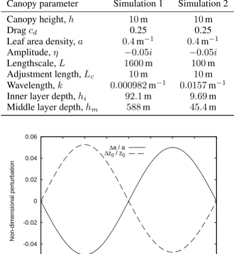
-0.06 -0.04 -0.02 0 0.02 0.04 0.06
-2 -1.5 -1 -0.5 0 0.5 1 1.5 2
Non-dimensional perturbation
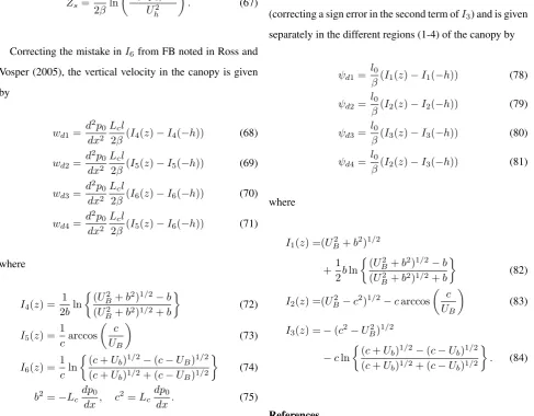
[image:12.595.56.295.89.211.2]x/L ∆a / a ∆z0 / z0
Figure 1.Non-dimensional perturbations in the canopy density,a(solid
line) and the roughness lengthz0(dashed line) as a function of horizontal
positionx/Lfor the two simulations presented here.
momentum is predominantly absorbed by the canopy. For
the long wavelength case this gives(kLc)2exp(βh/l0) =
0.0630and so the deep canopy contribution to the vertical
velocity is not important in the upper canopy. For the
shorter wavelength case(kLc)2exp(βh/l0) = 16.1and so
the vertical velocity field induced deep in the canopy is
likely to be important in the upper canopy solution. Figure 1
shows the non-dimensional canopy density and roughness
length perturbations for these cases as a function of the
horizontal coordinatex/L.
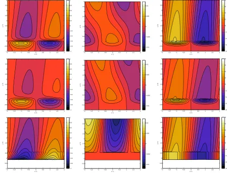
Figure 2 shows contour plots of the normalised
perturbation horizontal velocity u and vertical velocity
w for both the analytical solution and the numerical
model for the large wavelength (L= 1600m) case. There
is generally good qualitative and quantitative agreement
between the model in terms of the magnitude and phase of
the induced horizontal and vertical velocity perturbations,
although the analytical solution does appear to overestimate
the horizontal velocity perturbations compared to the
numerical model, while underestimating the maximum
vertical velocities at canopy top. There is some indication
of a difference in phase between the vertical velocity in the
analytical and numerical models atz/h∼4. This is likely
to be related to the turbulence scheme used and is discussed
in more detail in the following section. The analytical
solution gives strong gradients in the horizontal perturbation
at canopy top which are smoothed out in the numerical
model, partly due to numerical diffusion and partly due
to resolution. Note that although these look large on the
contour plots, the actual magnitudes are small compared
to the gradients in velocity in the background mean profile
since the perturbations are small.
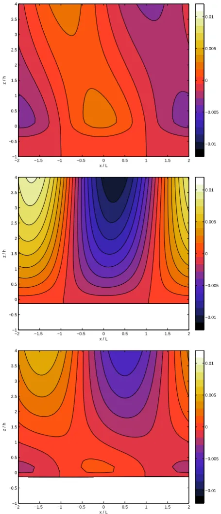
Figure 3 shows similar contour plots of the normalised
perturbation horizontal velocity uand vertical velocity w
for both the analytical solution and the numerical model for
the smaller wavelength (L= 100m) case. Note from table I
that in this case the inner layer thickness, hi= 9.69m is
comparable to the canopy depth and so much of the solution
plotted is the middle layer solution.
For the small wavelength case the advection terms at
canopy top are no longer negligible at leading order and
so the analytical model breaks down. As for flow over
a forested hill, reducing the wavelength results in an
increased gradient in the horizontal velocity variations (in
this case due to a more rapid change in canopy drag
rather than a large hill-induced pressure gradient), which in
turn increases the vertical velocity induced in the canopy.
This is most obviously seen by comparing the vertical
velocity in the upper canopy (note the different scales
compared to figure 2), which affects the induced pressure
field, and leads to the pressure gradient term becoming
important in the deep canopy. The canopy-induced shift
in the pressure gradient in turn leads to the strong shift
in phase of the perturbations in horizontal velocity in the
canopy which are observed in the numerical model. The
failure of the analytical model to account for the effects
of advection and the pressure gradient in the upper canopy
[image:12.595.55.295.92.353.2]x / L
z / h
−2 −1.5 −1 −0.5 0 0.5 1 1.5 2 −1 −0.5 0 0.5 1 1.5 2 2.5 3 3.5 4 −1 −0.8 −0.6 −0.4 −0.2 0 0.2 0.4 0.6 0.8 1
x / L
z / h
−2 −1.5 −1 −0.5 0 0.5 1 1.5 2 −1 −0.5 0 0.5 1 1.5 2 2.5 3 3.5 4 −0.01 −0.005 0 0.005 0.01
x / L
z / h
−2 −1.5 −1 −0.5 0 0.5 1 1.5 2 −1 −0.5 0 0.5 1 1.5 2 2.5 3 3.5 4 −8 −6 −4 −2 0 2 4 6 8
x / L
z / h
−2 −1.5 −1 −0.5 0 0.5 1 1.5 2 −1 −0.5 0 0.5 1 1.5 2 2.5 3 3.5 4 −1 −0.8 −0.6 −0.4 −0.2 0 0.2 0.4 0.6 0.8 1
x / L
z / h
−2 −1.5 −1 −0.5 0 0.5 1 1.5 2 −1 −0.5 0 0.5 1 1.5 2 2.5 3 3.5 4 −0.01 −0.005 0 0.005 0.01
x / L
z / h
[image:13.595.70.522.71.413.2]−2 −1.5 −1 −0.5 0 0.5 1 1.5 2 −1 −0.5 0 0.5 1 1.5 2 2.5 3 3.5 4 −8 −6 −4 −2 0 2 4 6 8
Figure 2.Contour plots of the normalised perturbation horizontal velocity,u/(U0η/κ)(left panels) and vertical velocity ,w/(U0η/κ)(right
panels) from the analytical solution (top), numerical model (middle) and the analytical solution of BXH (bottom). Results are shown for the case withL= 1600m.
phase shifts. The discontinuity in w at canopy top in
the analytical canopy solution is due the inclusion of the
contribution of the pressure gradient term in the canopy
vertical velocity expression, while this term is neglected
when matching to the SSL vertical velocity above. In
the regions of convergence strong vertical velocities are
generated for the short wavelength case (figure 3) and this
reflects the breakdown of the analytical solution for the
short wavelength case.
In both the canopy and roughness length analytical
models u and w are discontinuous at the inner layer
height,hi/h= 0.97, because the matching at this interface
is asymptotic (see sections 2.2.1 and 2.2.2). Since the
definition of the inner layer height is somewhat heuristic
and since in reality there is not a sharp interface between the
two layers this approach is physically and mathematically
reasonable. Blending the two solutions over some range of
heights would produce a smooth solution which might be
more realistic and would reflect the fact that physically the
transition between these two layers is not abrupt. On the
other hand this introduces some arbitrariness in the choice
of blending function and disguises the different behaviour
of the solutions in the different layers. For this reason no
blending has been done in the results presented here. It is
worth noting that this asymptotic matching is applied in
all the analytical models of this type for flow over hills
or heterogeneous terrain (e.g. BXH and FB) but is not
widely discussed. For long wavelength variations in terrain
or surface properties the inner and middle layer solutions
vary relatively smoothly and so the asymptotic matching
does not lead to significant discontinuities at the inner
layer height (figure 2). As the wavelength of the variations
decreases (figure 3) the inner layer solutions change more
x / L
z / h
−2 −1.5 −1 −0.5 0 0.5 1 1.5 2 −1 −0.5 0 0.5 1 1.5 2 2.5 3 3.5 4 −1 −0.8 −0.6 −0.4 −0.2 0 0.2 0.4 0.6 0.8 1
x / L
z / h
−2 −1.5 −1 −0.5 0 0.5 1 1.5 2 −1 −0.5 0 0.5 1 1.5 2 2.5 3 3.5 4 −0.1 −0.05 0 0.05 0.1 0.15
x / L
z / h
−2 −1.5 −1 −0.5 0 0.5 1 1.5 2 −1 −0.5 0 0.5 1 1.5 2 2.5 3 3.5 4 −5 −4 −3 −2 −1 0 1 2 3 4 5
x / L
z / h
−2 −1.5 −1 −0.5 0 0.5 1 1.5 2 −1 −0.5 0 0.5 1 1.5 2 2.5 3 3.5 4 −1 −0.8 −0.6 −0.4 −0.2 0 0.2 0.4 0.6 0.8 1
x / L
z / h
−2 −1.5 −1 −0.5 0 0.5 1 1.5 2 −1 −0.5 0 0.5 1 1.5 2 2.5 3 3.5 4 −0.1 −0.05 0 0.05 0.1 0.15
x / L
z / h
[image:14.595.71.522.69.417.2]−2 −1.5 −1 −0.5 0 0.5 1 1.5 2 −1 −0.5 0 0.5 1 1.5 2 2.5 3 3.5 4 −5 −4 −3 −2 −1 0 1 2 3 4 5
Figure 3.Contour plots of the normalised perturbation horizontal velocity,u/(U0η/κ)(left panels) and vertical velocity ,w/(U0η/κ)(right panels)
from the analytical solution (top), numerical model (middle) and the analytical solution of BXH (bottom). The thick black line in the top panels marks
the recirculation region. Results are shown for the case withL= 100m.
solution at the inner layer height do not agree so well. This
is in part because the inner layer height is less for small
wavelengths. For the analytical model developed here the
solution breaks down for small wavelengths, including the
case shown in figure 3, as the induced vertical velocities in
the canopy become sufficiently large that advection terms
cannot be neglected. It is therefore perhaps not surprising
that the solution is not as well behaved in this case.
Figure 3 is an example where the pressure gradient
induced in the canopy is sufficiently large to cause the
flow to separate. The streamline delineating the region of
separated flow is marked with a thick solid line in figure 3.
This can be calculated using the streamfunction given in
Appendix A. In this example the recirculation region is
relatively shallow. The numerical simulations do not exhibit
flow separation, largely because the numerical model has a
no-slip lower boundary condition which tends to reduce the
induced flow near the surface and inhibit flow separation.
4.2. Impact of the closure assumptions
The empirical relationship used to parameterize τxx and
τzz is worth discussing in further detail. Firstly, the
terms involving τxx and τzz are not important in the
leading order solutions for the velocity perturbations and
so these solutions are relatively insensitive to the turbulence
parameterization. Even a mixing length closure scheme will
give a reasonably accurate prediction of the shear stress
τ in the canopy and inner region and therefore get the
main induced flow pattern correct. The pressure field in
the canopy and inner region comes from the σ(1) term given by Eq. 55 however, which does depend on theτzz
term (the solution containsα3) and so will be sensitive to
The parameterization used is derived from observations
in the free boundary layer. A synthesis of different
observations over canopies is given in Finnigan (2000) and
shows that both τxx/τ and τzz/τ decrease through the
roughness sublayer (RSL) above the canopy, with values at
canopy top being about 35% smaller than the values above
the RSL. The ratios decrease further with depth into the
canopy. The parameterization used here does not take into
account this variation. Within the canopy theτxx andτzz
terms do not appear in the solution presented here and so
any decrease with height in the canopy is not important,
however in the inner region there is an error in the pressure
field associated with the overestimate inτzz.
If instead a mixing length model was used to
parameterizeτzzso that
τzz=lm2
dU dz
∂w
∂z (60)
then substitution of the inner layer solutions shows that
τzz/τ=O(δ) and so can be ignored in the solutions
presented here (i.e. settingα3= 0).
The exact error in the canopy and inner region pressure
field resulting from this will depend on the nature of
the canopy and its variability. Analysis of Eq. (55) does
show that the magnitude of the pressure field will be
approximately right ifα3 is set to zero, but there will be
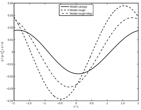
a significant shift in the phase of the pressure. Figure 4
show how the analytical canopy pressure field varies for
three different values of α3, and also the results with the
numerical model.
For the longer wavelength variation in canopy drag, the
analytical canopy solution withα3= 0(i.e. representing a
mixing length scheme) is in very good agreement with the
numerical model. Increasing values of α3 tend to lead to
a slight increase in the induced pressure field and a small
negative shift in the phase of the surface pressure. These
values cover the likely range of values above real canopies
based on observations and so give some indication of the
uncertainty due to the parameterization ofτzz.
−2 −1.5 −1 −0.5 0 0.5 1 1.5 2 −0.03
−0.02 −0.01 0 0.01 0.02 0.03
x / L
p / (
ρ
U
0
2ε
η
/
κ
)
α3 = 1.7
α3 = 1.13
α3 = 0.0
BXH Model canopy
−2 −1.5 −1 −0.5 0 0.5 1 1.5 2 −0.1
−0.05 0 0.05 0.1 0.15
x / L
p / (
ρ
U0
2ε
η
/
κ
)
α3 = 1.7
α3 = 1.13
[image:15.595.309.535.72.421.2]α3 = 0.0 BXH Model canopy
Figure 4.Normalised pressure field,p/(ρU2
0η/κ), within the canopy
as a function of horizontal position. Analytical results using the canopy
model are shown for three different values ofα3along with the analytical
results of BXH (withα3= 1.7) and the numerical results from the mixing
length numerical model. Results are for cases withL= 1600m (top) and
L= 100m (bottom).
For the smaller wavelength variation in canopy drag,
where vertical advection at canopy top is no longer
negligible, then the pressure field is much larger and
predominantly determined by the vertical velocity at canopy
top (the w(1)c terms in Eq. 55). In this case (bottom plot
of figure 4) the variation in the analytical surface pressure
field with α3 is much smaller. There is still a significant
phase and amplitude shift between the model and all the
analytical canopy solutions, which in this case is due to the
analytical model failing to represent the coupling between
the canopy and the boundary layer through the advection
terms. As in the case of flow over a forested hill (Finnigan
and Belcher 2004; Ross and Vosper 2005) this leads to a
downwind phase shift in the vertical velocity and pressure
It is not possible to say for certain that the analytical
solutions for the pressure field in the long wavelength
case with α3= 1.7 are accurate since we have no truth
to compare with. We know the first order numerical
model is not accurate in representing the τzz term
and there is no experimental data (field or laboratory)
current published with which the analytical results can be
compared. However, the good agreement between analytical
and numerical models ifα3= 0provides confidence in the
analysis. Confidence in the closure assumptions withα3=
1.7 comes from the fact that it produces good agreement
between the analytical solution of BXH and numerical
model results from a model with a second order turbulence
closure scheme which does accurately predict theτzzterm.
Although there has been some work testing second order
closure model for homogeneous canopy flows (e.g. Ayotte
et al.1999; Pinard and Wilson 2001) this has not yet been applied to inhomogeneous canopies, and so it is not possible
to do the same comparison as BXH between analytical
solution and second order numerical model for the present
problem.
5. Comparison with flow over a surface of variable
roughness
As illustrated in figures 2 and 3 the response of the boundary
layer to flow over a surface of variable roughness is very
different to that over a canopy of variable density. The
results over a rough surface (bottom panels) are obtained
using the analytical solution of BXH for the equivalent
roughness length
z1=
z0
(1 +ηeikx) (61)
and so the roughness parameter,M, in the BXH analytical
solution is equal toη. The form of the solution in the middle
layer and the outer layer is the same in each case, with only
the values of the constants B0,C0 andD0 differing. For
the longer wavelength change in canopy density (figure 2)
the solutions broadly agree for large z, although there is
a slight phase shift in the uandw fields. The agreement
is also reflected in the similar phase of the pressure fields
between the two analytical solutions (figure 4). In the shear
stress layer however the solutions show markedly different
behaviour. This difference is due to the fundamentally
different behaviour near the surface in the two cases. In
the canopy, the horizontal velocity perturbation is180◦out of phase with the canopy density variations since a denser
canopy tends to slow down the flow. Continuity shows that
the induced vertical velocity field has a phase90◦ ahead of the canopy density. Just above the canopy the velocity
perturbations are dominated by the canopy-induced flow
since u and w are continuous at canopy top. There is a
large phase shift inuandwacross the shear stress layer to
match the middle and outer layer solutions. In contrast, over
a rough surface there is no vertical velocity near the surface
and so the velocity perturbations are induced within the
inner surface and shear stress layers. An increase in canopy
density corresponds to a decrease in the roughness length
since the roughness length is proportional to the canopy
mixing length (see Eq. 4). Decreasing the roughness will
tend to increase the flow speed and so over a rough surface
the horizontal velocity perturbations will tend to be in phase
with the canopy density changes, the exact opposite of the
case where a canopy is included. Similarly the near-surface
vertical velocity over a rough surface is180◦ out of phase with that over a canopy. The phase of the perturbations are
relatively constant with height in the shear stress layer over
a rough surface.
As Hobson et al. (1999) and others have pointed out, varying only the roughness of a surface is not necessarily
realistic. In practice changes in roughness will also be
accompanied by changes in the roughness displacement
height, which will also impact on the near surface flow.
To investigate the impact of displacement height, results
from three different numerical simulations are presented
for the wide domain in figure 5. The first of these
simulations has the canopy modelled explicitly (top plot)
roughness (middle plot) and the third has a surface with
both roughness and displacement height varied (bottom
plot). The variations in canopy density, roughness and
displacement height are chosen to be equivalent so that
z0= (l/κ) exp(−κ/β)andd=l/κwherel= 2β3/(Ca).
Note that in the numerical model, due to the way the lower
boundary condition is coded, the variable displacement
height is actually modelled with a variable surface height.
As seen in the analytical solutions in figure 2, the model
demonstrates significant differences in behaviour between
the solution with an explicit canopy and the solution with
only a variable roughness length. Inclusion of the effects
of variable displacement height significantly alters the near
surface (i.e. canopy top) behaviour of the numerical model
and gives a vertical velocity field closer to that predicted
with an explicit canopy. There are however still significant
differences, particularly further above the surface. These
differences in the vertical velocity field above the canopy
mean that the induced surface pressure field (figure 6)
differs between the three runs.
Finally, it is interesting to compare the behaviour of
the two analytical solutions in the limit as the canopy
approaches a rough surface, i.e. the canopy density is large
so that flow into / out of the canopy is negligible. In this
limitkLc→0. To evaluate the constants in this limit recall
thatkLc→0⇒ζ0→0. Taking expansions of the Bessel
and Lommel functions for small arguments gives
K00∼ −
1
2log(ζ0), ζ0K 0
00∼ −
1 2,
S00∼ −
1 16iζ0
, ζ0S000 ∼
1 16iζ0
(62)
and on substituting these we obtain
A0→2δ, B0→ −
2κ2δ2
U(hi)
,
C0→ −2ikhmδ2
iκ2
U(hi)
, D0→ −
2κ2δ2
U(hi)
(63)
wherewc→0in the rough surface limit. In this limit these
canopy solution constants all tend to the same values as
x / L
z / h
−2 −1.5 −1 −0.5 0 0.5 1 1.5 2 −1
−0.5 0 0.5 1 1.5 2 2.5 3 3.5 4
−0.01 −0.005 0 0.005 0.01
x / L
z / h
−2 −1.5 −1 −0.5 0 0.5 1 1.5 2 −1
−0.5 0 0.5 1 1.5 2 2.5 3 3.5 4
−0.01 −0.005 0 0.005 0.01
x / L
z / h
−2 −1.5 −1 −0.5 0 0.5 1 1.5 2 −1
−0.5 0 0.5 1 1.5 2 2.5 3 3.5 4
[image:17.595.308.536.69.598.2]−0.01 −0.005 0 0.005 0.01
Figure 5.Contour plots of the normalised vertical velocity ,w/(U0η/κ),
from the numerical model for simulations with an explicit canopy of variable density (top), a surface with variable roughness (middle) and a surface with variable roughness and displacement height (bottom). Results
are shown for the case withL= 1600m.
the corresponding constant in the rough surface solution.
In the middle and outer layers the form of the solutions
in the same in both solutions and so if the constants agree
then the solutions are the same in the rough surface limit.
In the shear stress layer the solution foruover a canopy,