Neural language models with latent syntax
MSc Thesis(Afstudeerscriptie) written by
Daan van Stigt
(born August 17, 1992 in Amsterdam, The Netherlands)
under the supervision ofDr. Wilker Aziz, and submitted to the Board of Examiners in partial fulfillment of the requirements for the degree of
MSc in Logic
at theUniversiteit van Amsterdam.
Date of the public defense: Members of the Thesis Committee: May 24, 2019 Dr. Wilker Aziz (supervisor)
Dr. Caio Corro
Abstract
Acknowledgements
Contents
1. Introduction 8
2. Background 11
2.1. Syntax . . . 11
2.1.1. Constituents . . . 11
2.1.2. Categories . . . 12
2.1.3. Hierarchy . . . 13
2.1.4. Controversy . . . 14
2.2. Parsing . . . 14
2.2.1. Treebank . . . 16
2.2.2. Models . . . 16
2.2.3. Metrics . . . 18
2.3. Language models . . . 19
2.3.1. Models . . . 19
2.3.2. Data . . . 20
2.3.3. Metrics . . . 21
2.4. Neural networks . . . 21
2.4.1. Functions . . . 22
2.4.2. Optimization . . . 22
3. Recurrent Neural Network Grammars 24 3.1. Model . . . 24
3.1.1. Transition sytem . . . 25
3.1.2. Model . . . 26
3.2. Parametrization . . . 29
3.2.1. Stack encoder . . . 29
3.2.2. Composition function . . . 30
3.3. Training . . . 31
3.4. Inference . . . 31
3.4.1. Discriminative model . . . 31
3.4.2. Generative model . . . 32
3.5. Experiments . . . 33
3.5.1. Setup . . . 34
3.5.2. Results . . . 34
3.5.3. Analysis . . . 35
4. Conditional Random Field parser 40
4.1. Model . . . 41
4.2. Parametrization . . . 42
4.3. Inference . . . 42
4.3.1. Weighted parse forest . . . 43
4.3.2. Inside recursion . . . 44
4.3.3. Outside recursion . . . 46
4.3.4. Solutions . . . 47
4.4. Training . . . 49
4.4.1. Objective . . . 49
4.4.2. Speed and complexity . . . 50
4.5. Experiments . . . 51
4.5.1. Setup . . . 51
4.5.2. Results . . . 51
4.5.3. Proposal distribution . . . 52
4.5.4. Analysis . . . 52
4.6. Trees and derivations . . . 55
4.6.1. Derivational ambiguity . . . 55
4.6.2. Consequences . . . 56
4.6.3. Solutions . . . 56
4.6.4. Unrestricted parse forest . . . 57
4.6.5. Pruned parse forest . . . 58
4.7. Related work . . . 60
5. Semisupervised learning 62 5.1. Unsupervised learning . . . 63
5.1.1. Variational approximation . . . 63
5.1.2. Approximate posterior . . . 64
5.2. Training . . . 64
5.2.1. Gradients of generative model . . . 65
5.2.2. Gradients of inference model . . . 66
5.2.3. Variance reduction . . . 66
5.3. Experiments . . . 67
5.3.1. RNNG posterior . . . 67
5.3.2. CRF posterior . . . 68
5.4. Related work . . . 69
6. Syntactic evaluation 71 6.1. Syntactic evaluation . . . 71
6.1.1. Dataset . . . 72
6.1.2. RNNG . . . 73
6.2. Multitask learning . . . 75
6.2.1. Multitask objective . . . 75
6.3. Experiments . . . 77
6.3.1. Setup . . . 77
6.3.2. Results . . . 78
6.4. Related work . . . 81
7. Conclusion 83 7.1. Main contributions . . . 83
7.2. Future work . . . 84
A. Implementation 86 A.1. Data . . . 86
A.1.1. Datasets . . . 86
A.1.2. Vocabularies . . . 87
A.2. Implementation . . . 88
B. Semiring parsing 90 B.1. Hypergraph . . . 90
B.2. Semiring . . . 91
B.3. Semiring parsing . . . 92
B.3.1. Inside and outside recursions . . . 93
B.3.2. Instantiated recursions . . . 94
C. Variational inference 96 C.1. Score function estimator . . . 96
C.2. Variance reduction . . . 97
C.2.1. Control variate . . . 97
C.2.2. Baseline . . . 100
C.3. Optimization . . . 100
Notation
a,b, . . . Vectors over the reals,i.e.a2Rm.
A,B, . . . Matrices over the reals,i.e.A2Rm⇥n.
[a]i Vector indexing:[a]i2Rfor1im.
[a;b] Vector concatenation:a2Rm,b2Rn,[a;b]2Rm+n.
A B Hadamard product(A B)ij = (A)ij(B)ij.
X Finite vocabulary of wordsx.
Y(x) Finite set of treesyover a sentencex.
V(x) Finite set of labeled spansvover a sentencex. X, Y, . . . Random variables with sample spacesX,Y, . . . x A word fromX, outcome of random variableX. y A tree fromY(x), outcome of random variableY. xm
1 A sequence of wordshx1, . . . , xmifromXm, shorthand:x.
x<i The sequencexi1 1precedingxi.
PX Probability distribution.
pX Probability mass function.
p(x) ProbabilityP(X=x).
p✓,q Probability mass functions with emphasis on parameters.
E[g(X)] Expectation ofg(X)with respect to distributionPX.
H(X) Entropy of random variableX.
KL(q||p) Kullback-Leibler divergence between distributionsqandp.
⇤ Finite set of nonterminal labels.
A, B, . . . Nonterminal labels from⇤.
? Dummy label used for binarization, in⇤.
S† Special root label, not in⇤.
2A The powerset of setA.
1. Introduction
Perhaps the most basic yet profound task in probabilistic modelling of language is to assign probabilities to sentences—such probability distribution is called a language model. This thesis studies how such distributions can be extended to incorporate that which is not observed in words alone: the sentence’s syntactic structure.
In this thesis we are interested in distributions that assign probabilitiesp(x, y)topairs of observations—both the sentencexand its syntactic structurey. Rules of probability then gives us a language model for free because for any joint probability distribution
p(x) = X
y2Y(x)
p(x, y).
‘For free’, because for any combinatorial structure of any interest the sum overywill be daunting, and can generally be computed exactly only for models that factorizep(x, y) along significant independence assumptions. Approximations are in place when pis too expressive. The above marginalization is the core subject of this thesis: the spread of probabilityp(x)over the many probabilitiesp(x, y), each describing how sentencex and structurey cooccur. How does this spread makep a better model of sentencesx? How can we approximate the sum overy when the model p is too expressive? And how can we estimate probabilitiesp(x, y)when onlyxis ever observed?
We ask these questions for one joint model in particular: the recurrent neural network grammar (RNNG) [Dyer et al., 2016]. The RNNG models this joint distribution as a se-quential generation process that generates words together with their phrase structure. It merges generative transition-based parsing with recurrent neural networks (RNNs), factorizing the joint probability as the product of probabilities of actions in a transi-tion system that builds trees top-down. It makes no independence assumptransi-tions about this sequential process: at each step, the model can condition on the entire derivation constructed thus far, which is summarized by a syntax-dependent RNN.
model of language that can outperform RNN language models in terms of perplexity [Dyer et al., 2016] and on a targeted syntactic agreement task [Kuncoro et al., 2018].
The approximate marginalization is central in the application of the RNNG as lan-guage model, and the supervised learning requires annotated data. In this thesis we study this marginalization, to see if we can extend estimation to data without annota-tion.
Our central contribution is the introduction of a neural conditional random field (CRF) constituency parser that can act as an alternative approximate posterior for the RNNG. The CRF parser can be used as proposal model for a trained RNNG, but we also experiment with the CRF as approximtate posterior in variational learning of the RNNG, in which we jointly learn the RNNG and CRF by optimizing a lower bound on the marginal log-likelihood. This opens the door to semisupervised and unsupervised learning of the RNNG. The CRF formulation of the parser allows the exact computation of key quantities involved in the computation of the lower bound, and the global nor-malization provides a robust distribution for the sampling based gradient estimation.
To evaluate how the joint formulation differentiates the RNNG from neural language models that model onlyxwe perform targeted syntactic evaluation of these models on the dataset of [Marvin and Linzen, 2018]. A competitive alternative to the full joint model of the RNNG are RNN language models that receive syntactic supervision dur-ing traindur-ing in the form of multitask learndur-ing. We compare the RNNG to these models, as well as to an RNN language that is trained without any additional syntactic super-vision.
The organization of this thesis is as follows.
Chapter 2 In this chapter we describe the background to this thesis. We first describe the fundamentals of phrase structure, motivating why we might need it for a characterization of language. We then describe syntactic parsing, emphasizing the difference between globally and locally normalized models. Similarly, we describe language modelling, emphasizing relevant related models. We conclude with a review of the neural networks used in this thesis.
Chapter 3 In this chapter we review the RNNG. We describe the exact probabilistic model, the neural parametrization, the supervised training, and the approximate inference. We report results with our own implementation, and analyze the ap-proximate inference with the discriminative RNNG.
the way our model deals withn-ary trees which leads to derivational ambiguity. The derivational ambiguity is not a direct problem for the application of the CRF as a parser, but does become one in its application as posterior distribution in the approximate inference. We provide solutions in the form of alternative inference algorithms, and preliminary results show that these are easy to implement and resolve the ambiguity.
Chapter 5 This chapter contains part two of our core contribution: we address the semisupervised and unsupervised learning of the RNNG, focussing on the CRF as approximate posterior. We derive a variational lower bound on the marginal log likelihood and show how this can be optimized by sampling based gradient estimation. We perform experiments with semisupervised, and unsupervised ob-jectives, for labeled and unlabeled trees, but a full exploration of the CRF in this role is halted by the derivational ambiguity. Preliminary results with unlabeled trees suggest the potential of this approach for unsupervisedn-ary tree induction, and we formulate future work towards this goal.
Chapter 6 In the final chapter we perform syntactic evaluation using the dataset of Marvin and Linzen [2018]. We compare the supervised RNNG with RNN lan-guage models that are trained with a syntactic side objective, a type of multitask learning. We additionally propose a novel side objective inspired by the scoring function of the CRF.
Conclusion We summarize our work and list our main contributions, and finish with suggestions for future work that departs from where our investigation leaves off.
2. Background
This section provides background on the four topics that are combined in this thesis: syntax, parsing, language modelling, and neural networks.
2.1. Syntax
We first introduce some concepts relating to syntax that are relevant for this thesis. In particular, we introduce the notion of aconstituent, and the hierarchical organization of constituents in a sentence as described byphrase-structure grammars. The aim is to provide a succinct and compelling answer to the question: why should we care about constituency structure when modelling language?
Our exposition primarily follows Huddleston and Pullum [2002], a well established reference grammar of the English language that is relatively agnostic with respect to theoretical framework, with some excursions into Carnie [2010] and Everaert et al. [2015], which are less language-specific but rooted more in a particular theoretical framework1. We take the following three principles from Huddleston and Pullum [2002] as guiding:
1. Sentences consist of parts that may themselves have parts. 2. These parts belong to a limited range of types.
3. The constituents have specific roles in the larger parts they belong to.
To each principle we now dedicate a separate section.
2.1.1. Constituents
Sentences consist of parts that may themselves have parts. The parts are groups of words that function as units and are calledconstituents. Consider the simple sentence A bird hit the car. The immediate constituents area bird(the subject) andhit the car(the predicate). The phrasehit the carcan be analyzed further as containing the constituent the car. The ultimate constituents of a sentence are the atomic words, and the entire analysis is called the constituent structure of the sentence. This structure can be indi-cated succinctly with the use of brackets
(1) [ A bird ] [ hit [ the car ] ]
or less succinctly as a tree diagram. Evidence for the existence of such constituents
·
·
·
car the hit ·
bird A
can be provided by examples such as the following, which are called constituent tests [Carnie, 2010]. Consider inserting the adverbapparentlyinto our example sentence, to indicate the alleged status of the event described in the sentence. In principle there are six positions available for the placement ofapparently(including before, and after the sentence). However, only three of these placements are actually permissible:2
(2) a. Apparentlya bird hit the car. b. *Anapparentlybird hit the car. c. A birdapparentlyhit the car. d. *A bird hitapparentlythe car. e. *A bird hit theapparentlycar. f. A bird hit the car,apparently.
Based on the bracketing that we proposed for this sentence we can formulate a general constraint: the adverb must not interrupt any constituent. Indeed, this would explain why apparently cannot be placed anywhere inside hit the car and not between a and bird. For full support, typically, results from many more such test are gathered, and in general these tests can be much more controversial than in our simple example [Carnie, 2010].
2.1.2. Categories
The constituents of a sentence belong to a limited range of types that form the set of syntactic categories. Two types of categories are distinguished: lexical and phrasal. The lexical categories are also known as part-of-speech tags. A tree can be represented in more detail by adding lexical (D, N, V) and phrasal categories (S, NP, VP). In this
S
VP
NP
N
car D
the V
hit NP
N
bird D
A
example, the noun (N)caris the head of the noun phrase (NP)the car, while the head of the larger phrasehit the car is the verb (V)hit, making this larger constituent averb phrase(VP). The whole combined forms a sentence (S).
2.1.3. Hierarchy
The constituents have specific roles in the larger parts they belong to. This structure provides constraints that are not explainable from the linear order of the words them-selves [Everaert et al., 2015]. Consider for instance the following example of the syn-tactic behaviour ofnegative polarity items(NPIs) from Everaert et al. [2015]. A negative polarity item is, to first approximation, a word or group of words that is restricted to negative context [Everaert et al., 2015].3 Take the behaviour of the wordanybody: (3) a. The talk I gave didnotappeal toanybody.
b. *The talk I gave appealed toanybody.
c. *The talk I didnotgive appealed toanybody.
From sentences (a) and (b) we might formulate the hypothesis that the wordnotmust linearly precede the wordanybody, but a counter example refutes this hypothesis: sen-tence (c) is also not grammatical. Instead—it is argued—the constraints that govern this particular pattern depend on hierarchical structure: the wordnotmust ‘structurally pre-cede’ the word anybody[Everaert et al., 2015]. Figure shows the constituent structure of both sentences. The explanation goes as follows: “In [the left tree] the hierarchical structure dominatingnot also immediately dominates the hierarchical structure con-taininganybody. In [the right tree], by contrast,notsequentially precedesanybody, but the triangle dominating not fails to also dominate the structure containing anybody.” [Everaert et al., 2015].
Examples adapted from Everaert et al. (TICS 2015)
containing anybody. (This structural configuration is called c(onstituent)-command in the linguistics literature [31].) When the relationship between not and anybody adheres to this structuralconfiguration,thesentenceiswell-formed.
Insentence(3),bycontrast,notsequentiallyprecedesanybody,butthetriangledominatingnot inFigure1Bfailstoalsodominatethestructurecontaininganybody.Consequently,thesentence isnotwell-formed.
Thereadermayconfirmthatthesamehierarchicalconstraintdictateswhethertheexamplesin (4–5)arewell-formed ornot, wherewe have depicted thehierarchical sentencestructure in terms ofconventionallabeled brackets:
(4) [S1[NPThebook[S2Ibought]S2]NPdidnot[VP appealto anyone]VP]S1
(5) *[S1[NPThe book[S2Ididnotbuy]S2]NP[VPappealedtoanyone]VP]S1
Onlyinexample(4)doesthehierarchicalstructurecontainingnot(correspondingtothesentence ThebookIboughtdidnotappealtoanyone)alsoimmediatelydominatetheNPIanybody.In(5) notisembeddedinatleastonephrasethatdoesnotalsoincludetheNPI.So(4)iswell-formed and(5)isnot,exactlythepredictedresultifthehierarchicalconstraintiscorrect.
Evenmorestrikingly,thesameconstraintappearstoholdacrosslanguagesandinmanyother syntacticcontexts.NotethatJapanese-typelanguagesfollowthissamepatternifweassume thattheselanguageshavehierarchicallystructuredexpressionssimilartoEnglish,butlinearize thesestructuressomewhatdifferently–verbscomeattheendofsentences,andsoforth[32]. Linearorder,then, shouldnotenterintothesyntactic–semantic computation[33,34].Thisis ratherindependentofpossibleeffectsoflinearlyinterveningnegationthatmodulateacceptability inNPIcontexts[35].
TheSyntax ofSyntax
Observe anexampleas in(6):
(6) Guesswhichpoliticianyourinterestin clearlyappealsto.
Theconstructionin(6)isremarkablebecauseasinglewh-phraseisassociatedboth
withtheprepositionalobjectgapoftoandwiththeprepositionalobjectgapofin,asin
(7a).Wetalkabout‘gaps’becauseapossibleresponseto(6)mightbeasin(7b):
(7) a. Guesswhichpoliticianyourinterest inGAPclearlyappealstoGAP.
b. responseto(7a):Your interestinDonaldTrumpclearlyappealstoDonaldTrump
(A) (B)
X X
X X X X
The book X X X The book X appealed to anybody
did not
that I bought appeal to anybody that I did notbuy
Figure 1. Negative Polarity.(A)Negative polaritylicensed:negative element c-commandsnegative polarityitem. (B)
Generalization:
Negativepolaritynotlicensed.not
Negativemust “structurally precede”
elementdoesnotc-commandnegativepolarityitem.anybody
Language is hierarchical
The talk
I gave
did not
appeal to anybody
appealed to anybody The talk
I did not give
Examples adapted from Everaert et al. (TICS 2015)
containing anybody. (This structural configuration is called c(onstituent)-command in the linguistics literature [31].) When the relationship between not and anybody adheres to this structuralconfiguration,thesentenceis well-formed.
Insentence(3),bycontrast,notsequentiallyprecedesanybody,butthetriangledominatingnot inFigure1Bfailstoalsodominatethestructurecontaininganybody.Consequently,thesentence isnotwell-formed.
Thereadermayconfirmthatthesamehierarchicalconstraintdictateswhethertheexamplesin (4–5) are well-formedor not,where wehavedepicted the hierarchicalsentencestructure in termsofconventionallabeledbrackets:
(4) [S1[NPThebook[S2Ibought]S2]NPdidnot[VPappealtoanyone]VP]S1
(5) *[S1[NPThebook[S2Ididnotbuy]S2]NP[VPappealedtoanyone]VP]S1
Onlyinexample(4)doesthehierarchicalstructurecontainingnot(correspondingtothesentence ThebookIboughtdidnotappealtoanyone)alsoimmediatelydominatetheNPIanybody.In(5) notisembeddedinatleastonephrasethatdoesnotalsoincludetheNPI.So(4)iswell-formed and(5)isnot,exactlythepredictedresultifthehierarchicalconstraintis correct.
Evenmorestrikingly,thesameconstraintappearstoholdacrosslanguagesandinmanyother syntacticcontexts.NotethatJapanese-typelanguagesfollowthissamepatternifweassume thattheselanguageshavehierarchicallystructuredexpressionssimilartoEnglish,butlinearize thesestructuressomewhatdifferently–verbscomeattheendofsentences,andsoforth[32]. Linearorder,then,shouldnotenterinto thesyntactic–semantic computation[33,34].This is ratherindependentofpossibleeffectsoflinearlyinterveningnegationthatmodulateacceptability inNPIcontexts [35].
TheSyntaxofSyntax
Observeanexampleasin(6):
(6) Guess whichpoliticianyourinterestinclearlyappealsto.
Theconstructionin(6)isremarkablebecauseasinglewh-phraseis associatedboth withtheprepositionalobjectgapoftoandwiththeprepositionalobjectgapofin,asin (7a).Wetalkabout‘gaps’becauseapossibleresponseto(6)mightbeasin(7b):
(7) a. GuesswhichpoliticianyourinterestinGAPclearlyappealstoGAP.
b. responseto(7a):YourinterestinDonaldTrumpclearlyappealstoDonaldTrump
(A) (B)
X X
X X X X
The book X X X The book X appealed to anybody did not
that I bought appeal to anybody that I did notbuy
Figure 1.Negative Polarity. (A)Negative polarity licensed:negativeelementc-commandsnegativepolarity item. (B)
Generalization:
Negativepolaritynotlicensed.not
Negativemust “structurally precede”
elementdoesnotc-commandnegativepolarityitem.anybody
-
many theories of the details of structure
-
the psychological reality of structural sensitivty
is
not
empirically controversial
-
much more than NPIs follow such constraints
Language is hierarchical
The talk
I gave
did not
appeal to anybody
appealed to anybody
The talk
[image:13.595.103.495.474.557.2]I did not give
Figure 2.1.: Dependance on hierarchical structure of negative polarity items. Left shows the wordanybodyin the licensing context ofnot. Right shows the ungram-matical sentence where the word is not. Figure taken from Everaert et al. [2015]. The triangles indicate substructre that is not further explicated.
3More generaly, they are words that need to be licensed by a specific licencing context[Giannakidou,
2011].
2.1.4. Controversy
Theoretical syntax is rife with controversy, and wildly differing viewpoints exist. In fact, for each point made in our short discussion the exact opposite point has been made as well:
• Work in dependency grammar and other word-based grammar formalisms de-parts from the idea that lexical relations between individual words are more fun-damental than constituents and their hierarchical organization [Tesni`ere, 1959, Nivre, 2005, Hudson, 2010], and dispenses with the notion of constituents alto-gether.
• A recurring cause of controversy is the question whether hierarchical structure needs to be invoked in linguistic explanation. That is, whether the kind of anal-ysis we presented with embedded, hierarchically organized constituents is really fundamental to language. Frank et al. [2012] argue for instance that a shallow analysis of sentences into immediate constituents with linear order but no hier-achical structure4 is sufficient for syntactic theories, a claim that is vehemently rejected by Everaert et al. [2015].
• Research in cognitive neuroscience and psycholinguistics shows that human sen-tence processing is hierachical, giving evidence that processing crucially depends on the kind of structures introduced in the sections above [Hale, 2001, Levy, 2008, Brennan et al., 2016]. However, research also exists that shows that purely linear predictors are sufficient for modeling sentence comprehension, thus showing the exact opposite to be true [Conway and Pisoni, 2008, Gillespie and Pearlmutter, 2011, Christiansen et al., 2012, Gillespie and Pearlmutter, 2013, Frank et al., 2012]. Our work, however, takes a pragmatic position with respect to such questions: syn-tax, we assume, is whatever our dataset says it is. And to some degree, the question whether language is hierachical or linear is a question that this thesis engages with from a statistical and computational standpoint.
2.2. Parsing
Parsing is the task of predicting a treeyfor a sentencex. Probabilitic parsers solve this problem by learning a probabilistic model p that describes a probability distribution overallthe possible parsesyof a sentencex. This distribution quantifies the uncertainty over the syntactic analyses of the sentence, and can be used to make predictions by find-ing the trees with highest probability. A further benefit of the probabilistic formulation is that the uncertainty over the parses can be determined quantitatively by computing the entropy of the distribution, and qualitatively by obtaining samples from the dis-tribution. This section describes the form that such probabilistic models take, and the data from which they are estimated.
S . VP NP-PRD PP NP worlds all of NP worst the was SBAR-NOM-SBJ S VP NP-TMP Friday happened NP-SBJ *T*-1 WHNP-1 What
(a) Original Penn Treebank tree.
S . VP NP PP NP worlds all of NP worst the was SBAR S VP NP Friday happened WHNP What
(b) Function tags and traces removed.
S ? ? . VP NP PP NP ? worlds ? all ? of NP ? worst ? the ? was SBAR S+VP NP Friday ? happened WHNP What
(c) Converted to normal form using a dummy label?.
S10 0 ?10 3 ?10 9 . VP9 3 NP9 4 PP9 6 NP9 7 ?9 8 worlds ?8 7 all ?7 6 of NP6 4 ?6 5 worst ?5 4 the ?4 3 was SBAR3 0 S+VP3 1 NP3 2 Friday ?2 1 happened WHNP1 0 What
[image:15.595.166.427.94.537.2](d) In normal form with spans.
2.2.1. Treebank
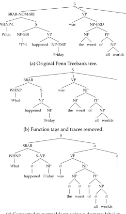
A treebank is a collection of sentences annotated with their grammatical structure that allows the estimation of statistical parsings models. The Penn Treebank [Marcus et al., 1993] is such a collection, consisting of sentences annotated with their constituency structure. Figure 2.2a shows an example tree from this dataset and figure 2.2b shows the tree after basic processing5. Some parsing models require trees to be innormal form: fully binary, but with unary branches at the terminals. The CRF parser introduced in chapter 4 is an example of such a model. Figure 2.2c shows the result of the (invertible) normalization that we use. The tree is obtained by right branching binarization, intro-ducing a special dummy label?in the process that can be treated as any other label in tree. Annotating the labels with left and right endpoints of the words they span results in the tree in figure 2.2d.
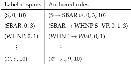
A tree can be factorized into its parts: we can think of tree as a set oflabeled spans, or as a set of anchored rules. A labeled span is a triple(A, i, j) of a syntactic label A from a labelset⇤together with the left and right endpointsi,jthat the label spans. An anchored ruleis a triple(r, i, j)or four-tuple(r, i, k, j), containing a rulerin normal form with span endpointsi,j, and a split-pointkof the left and right child whenr is not a lexical rule. Consider these two representations of the tree in figure 2.2d given in table 2.1. These different factorizations will become relevant in chapter 4 when formulating the probabilistic model.
Labeled spans Anchored rules (S, 0, 10) (S!SBAR?, 0, 3, 10)
(SBAR, 0, 3) (SBAR!WHNP S+VP, 0, 1, 3) (WHNP, 0, 1) (WHNP!What, 0, 1)
... ...
[image:16.595.185.408.394.503.2](?, 9, 10) (?!., 9, 10)
Table 2.1.: Two representations of the tree in 2.2d.
2.2.2. Models
The probabilistic model of a parser can be discriminative, describing the conditional probability distributionp(y | x), orgenerative, describing the joint distributionp(x, y). The form that the model takes is largely dictated by the algorithm used to build the parses.
Transition-based methods formulate parsing as a sequence of shift-reduce decisions made by a push-down automaton that incrementally builds a tree. The design of the
5This removes the functional tags and annotation of argument structure introduced in version 2 of the
transition system determines whether the tree is constructed bottom-up, top-down,6or otherwise, and determines whether the trees need to be in normal form. The proba-bilistic model is defined over the sequences of actions, and the probability distribution typically factorizes as the product of conditional distributions over the next action given the previous actions. This makes it a directed model that islocally normalized.7
Definition 2.2.1. A probalistic modelpover sequencesa2Anislocally normalizedif
p(a) =
n
Y
i=1
p(ai |a<i)
=
n
Y
i=1
(a<i, ai)
Z(a<i)
,
whereZ(a<i) = Pa2A (a<i, a)is a local normalizer and is a nonnegative scoring
function: (a<i, ai) 0for alla<iandai.
Such a model is discriminative when the actions only build the tree, but can be made generative when word prediction is included in the action set.
Chart based parsing, on the other hand, factorizes trees along their parts, and defines the probabilistic model over the shared substructures. Representing the model as the product of local parts greatly reduces the number of variables required to specify the full distribution, and allows the use of dynamic programming for efficient inference. Discriminitive models based on conditional random fields (CRFs) [Lafferty et al., 2001] follow this factorization: local functions independently predict scores for the parts, and the product of this score is normalizedgloballyby a normalizer that sums over the ex-ponential number structures composable from the parts.
Definition 2.2.2. A probalistic modelpover sequencesa2Anisglobally normalizedif p(a) = (a)
Z ,
where Z = Pa2An (a) is a global normalization term, and (a) 0 for all a. To allow efficient computation of the normalizerZ, the function typically factors over parts—orcliques—ofaas the product of local potentitals (a) =QC2C C(aC), where
C✓2{1,...,n}contains sets of indices anda
C :={ai}i2C. The choice of parts depends on
the model and determines the feasibility of the sum computingZ.
Generative chart-based models, instead, estimate rule probabilities directly from a treebank. The probability of a tree is computed directly as the product of the probabili-ties of the rules that generate it, thus requiring no normalization.8
6Post-order and pre-order, respectively.
7With the exception of those approaches that instead define a conditional random field over the action
sequences [Andor et al., 2016], in which case the model is defined over the globally normalized action sequences.
8In fact, this makes generative chart-based models directed, locally normalized models: they generate
Either method have their advantages and disadvantages. The transition-based meth-ods are fast, running in time linear in the sequence length, and allow arbitrary features that can condition on the entire sentence and the partially constructed derivation. How-ever, directed models with local normalization are known to suffer from the problem of label bias [Lafferty et al., 2001], and conditioning on large parts of the partial deriva-tions prohibits exact inference, so that decoding can be done only approximately, either with greedy decoding or with beam search. The chart based methods, on the other hand, allow efficient exact inference, and the global training objective that results from the global normalization receives information from all substructures. The method is much slower, however, running in time cubic in the sentence length for normal form trees9and linear in the size of the grammar10, and the strong factorization of the struc-ture, which makes the exact inference tractable, also means that features can condition only on small parts instead of large substructures.
A general challenge for sequential transition based models, related to the problem of label bias, is that their training is highly local: during training the models are only ex-posed to the individual paths that generate the example tree, which is a mere fraction of all the possible paths that the model is defined over.11 Compare this with a glob-ally normalized model, where the factorization over parts lets the model learn from an example tree about all the trees that share substructure.
In this thesis we investigate models where the scoring function , or its factorized version , is implemented with neural networks. Chapter 3 describes a locally normal-ized transition-based model that has a discriminative and generative formulation, and chapter 4 introduces a globally normalized, discriminative chart-based parser.
2.2.3. Metrics
The standard evaluation for parsing is the Parseval metric [Black et al., 1991], which measures the number of correctly predicted labeled spans. The metric is defined as the harmonic mean, orF1 measure, of the labelling recallRand precisonP:
F1= 2P R
P +R. (2.1)
Let R be the set of labeled spans of the gold reference trees, and letP be the set of labeled spans of the predicted trees. The recall is the fraction of reference spans that
9With greater exponents for trees that are not in normal form. 10Giving a total time complexity ofO(n3
|G|), whereGis the set of normal form rules of the grammar.
11One way to answer to this challenge is to use use a dynamic oracle during training [Goldberg and
were predicted
R= |R\P| |R| ,
and the precision is the fraction of the predicted spans that is correct
P = |R\P| |P| .
The cannonical implementation of the Parseval metric is EVALB[Sekine and Collins, 1997].
2.3. Language models
A language model is a probability distribution over sequences of words. There are many ways to design such a model, and many datasets to estimate them from. This section focusses on those that are relevant to the models in this thesis.
2.3.1. Models
A language model is a probabilistic modelpthat assigns probabilities to sentences, or more formally, to sequencesx2X⇤ of any length over a finite vocabulary. Factorizing
the probability of a single sequencex2Xmover its timesteps gives the directed model:
p(x) =
m
Y
i=1
p(xi |x<i). (2.2)
This distribution can be approximated by lower order conditionals that condition on smaller, fixed-size, history, by making the Markov assumption assumption that
p(xi|x<i) =p(xi |xii j1 1).
This is the approach taken byn-gram language models. The lower order conditionals can be estimated directly by smoothing occurence counts [Kneser and Ney, 1995, Chen and Goodman, 1999], or they can be estimated by locally normalized scores (xii j1 1, xi),
given by a parametrized function . This function can be log-linear or a non-linear neu-ral network [Rosenfeld, 1996, Bengio et al., 2003]. The lower order approximation can also be dispensed with, making the model more expressive, but the estimation problem much harder. Language models based on recurrent neural networks (RNNs) follow this approach by using functions that compute scores (x<i, xi) based on the entire
current state of the art [Zaremba et al., 2014, Jozefowicz et al., 2016, Melis et al., 2017].12 Other neural network architectures based on convolutions [Kalchbrenner et al., 2014] and stacked feedforward networks with ‘self-attention’ [Vaswani et al., 2017] have been succesfully applied to language modelling with unbounded histories as well.
Alternatively, a language model can be obtained by marginalizing a structured latent variablehin a joint modelp(x, h):
p(x) = X
h2H
p(x, h). (2.3)
The structure of hallows this joint distribution to be factorized in a ways very much unlike that of equation 2.2. Such language models are defined for example by a Proba-bilistic Context Free Grammar (PCFG), in which casehis a tree, and a Hidden Markov Model (HMM), in which case h is a sequence of tags. The strong independence as-sumptions of these models allows the marginalization to be computed efficiently, but also disallows the models to capture arbitrary dependencies in x, which is precisely what we want from a language model. The recurrent neural network grammar (RNNG) [Dyer et al., 2016] model introduced in chapter 3 also defines a language model through a joint distribution, but that model is factorized as a sequential generation process over both the structurehand the sequencex, which makes it a competitive language model, but at the price of losing efficient exact marginalization.
This thesis focusses on language models that incorporate syntax. The models have precedents. Most directly related to our discussion are: language models obtained from top-down parsing with a PCFG [Roark, 2001]; syntactic extensions ofn-gram models with count-based and neural network estimation [Chelba and Jelinek, 2000, Emami and Jelinek, 2005]; and a method that is reminiscent ofn-gram methods, but based on arbi-trary overlapping tree fragments [Pauls and Klein, 2012].
2.3.2. Data
Language models enjoy the benefit that they require no labeled data; any collection of tokenized text can be used for training. In this work we focus on English language datasets. The sentences in the Penn Treebank have long been a popular dataset for this task. More recently has seen the introduction of datasets of much greater size, such as the One Billion Word Benchmark [Chelba et al., 2013] that consists of news articles, and datasets that focus on long-distance dependencies, such as the Wikitext datasets [Merity et al., 2016] that consists of Wikipedia articles grouped into paragraphs.
12Although recent work shows that the effective memory depth of RNN models is much smaller than the
unbounded history suggests: Chelba et al. [2017] show that, in the perplexity they assign to test data, an RNN with unbounded history can be approximated very well by an RNN with bounded history. To be precise: a neuraln-gram language model, with the fixed-size history encoded by a bidirectional RNN, is equivalent to an RNN with unbounded history forn= 13, and to an RNN that is reset at the
2.3.3. Metrics
The standard metric to evaluate a language model is the perplexity per token that it assigns to held out data. The lower the perplexity, the better the model. Perplexity is an information theoretic metric that corresponds to an exponentiated estimate of the model’s entropy normalized over number of predictions, measured in nats, and was introduced for this purpose by Jelinek [1997]13. The metric can be interpreted as the average number of guesses needed by the model to predict each word from its left context.
Definition 2.3.1. Theperplexity of a language model p on a sentencex of length mis defined as
exp
(
1
mlogp(x)
)
.
The perplexity on a set of sentences {x(1), . . . , x(N)} is defined as the exponentiated mean over all words together:
exp
(
1 M
N
X
n=1
logp(x(n))
)
,
whereM =PNn=1mnis the sum of all the sentence lengthsmn.
The appeal of perplexity is that it is an aggregate metric, conflating different causes of succes when predicting the next word. This conflation is also its main shortcom-ing, making it hard to determine whether the model has robustely learned high-level linguistic patterns such as those described in syntactic and semantic theories. For this reason, alternative methods have been proposed to evaluate language models: evalu-ation with adversarial examples [Smith, 2012]; prediction of long distance subject-verb agreement [Linzen et al., 2016]; and eliciting syntactic acceptability judgments [Marvin and Linzen, 2018]. Chapter 6 discusses these alternatives in greater detail, and demon-strates evalution with the method proposed in [Marvin and Linzen, 2018].
2.4. Neural networks
In this thesis we use neural networks to parametrize probability distributions. We con-sider a neural network an abstraction that denotes a certain type of parametrized dif-ferentiable function. We describe the functions used in this thesis, and describe how they are optimized using stochastic gradients.
2.4.1. Functions
Letxbe a word from a finite vocabularyX, and letxandybe vectors in respectively RnandRm.
Definition 2.4.1. Aword embeddingis vector representation of a word, assigned by an embeding function E that takes elements fromX toRn:
x=E(x).
The function can be a simple lookup table, or a more elaborate function that depends for example on the orthography of the word.
Definition 2.4.2. Afeedforward neural network is a parametrized function FFNfromRn
toRm:
y=FFN(x).
Internally, the function computes stacks of affine transformations followed by an ele-mentwise application of a nonlinear function. The number of repetitions of these appli-cations is refered to as the number of layers of the network.
Definition 2.4.3. Arecurrent neural network(RNN) is a parametrized function RNNthat takes a sequence of vectorsxk
1 = [x1,x2, . . . ,xk], each inRn, and produces a sequence
of output vectors[y1,y2, . . . ,yn]each inRm:
[y1,y2, . . . ,yk] =RNN(xk1).
Each vector yi is a function of the vectors [x1,x2, . . . ,xi], for which reason we refer
to the vectoryi as a context-dependentencoding of the vectorxi. An RNNcan be
ap-plied to the input sequence in reverse. This makes each yi a function of the vectors
[xi,xi+1, . . . ,xk]. We denote the output of the forward direction withf and the output
of the backward direction withb.
Definition 2.4.4. An RNN isbidirectionalwhen it combines the output of an RNN that runs in the forward direction, with the output of an RNN that runs in the backward direction. Combining their output vectors by concatenation gives for each position a vectorhi= [fi;bi]that is a function of the entire input sequence.
Definition 2.4.5. An LSTM [Hochreiter and Schmidhuber, 1997] is a particular way to implement the internals of the RNN function. It is the only type of RNN used in this work, and we use the two names exchangeably.
2.4.2. Optimization
optimized to find a maximum of anobjectivefunctionL using gradients. With neural networks, the functionLwill be highly nonconvex, in which case we can at most hope to find✓that give a good local optimum ofL(i.e. satisfyingr✓L(✓) = 0). Our
proto-typical objective is to optimize the log likelihood of a set of independent observations D={x(n)}Nn=1:
L(✓) =
N
X
n=1
logp✓(x(n)).
We perfom iterative parameter updates, obtaining new parameters✓(t+1) at timestep t+ 1from parameters✓(t)at timesteptusing the update rule
✓(t+1) =✓(t)+ (t)r✓(t)L(✓(t)),
where the value (t) is a time-indexed learning rate. We replacer
✓L(✓)with an
unbi-ased estimate
N K
K
X
k=1
r✓logp✓(x(k)),
where {x(1), . . . , x(K)} are sampled uniformly fromD, making our optimization pro-cedure stochastic. This set of data samples is referred to as a minibatch. This works because for and indexsdistributed uniformly between 1 andN the gradients equals an expectation
r✓L(✓) =NE
h
r✓logp✓(x(s))
i
.
Under certain conditions on the learning rate (t)this method is guaranteed to converge to a local optimum [Robbins and Monro, 1951]. For the computation ofr✓logp✓(x)we
3. Recurrent Neural Network Grammars
This chapter describes the Recurrent Neural Network Grammar (RNNG), a probabilis-tic model of sentences with phrase structure introduced by Dyer et al. [2016]. The model has a discriminative and generative formulation, but both are based on a shift-reduce transition system that builds trees in top-down order and define locally normalized probability distributions over action sequences. While the discriminative model is a constituency parser, the generative model is a joint model that can be evaluated both as constituency parser and as language model. The strength of both models lies in their unbouded history: at each step the model can condition on the entire derivation con-structed thus far. This derivation is summarized by a syntax-dependent recurrent neu-ral networks. This parametrization without independence assumptions, however, does preclude the use of exact inference—for example based on dynamic programming—but approximate inference based on greedy decoding and importance sampling provides tractable alternatives.
In this chapter:
• We describe the discriminative and generative formulations of the RNNG in de-tail.
• We describe the approximate inference algorithms that allow the RNNG to be used as parser and as language model.
• We implement the models and reproduce the results of Dyer et al. [2016].
3.1. Model
3.1.1. Transition sytem
Both RNNG models use a transition system crafted for top-down tree generation. The discriminative transition system has three actions:
• OPEN(X) opens a new nonterminal symbol X in the partially constructed tree.
• SHIFTmoves the topmost wordxfrom the buffer onto the stack.
• REDUCE closes the open constituent by composing the symbols in it into a single item representing the content of the subtree. This allows nodes with an arbitrary number of children.
How these actions work to build a tree is best illustrated with an example derivation.
Example 3.1.1. (Discriminative transition system) The following table shows the con-secutive states of the parser that produces the gold tree for input sentenceThe hungry cat sleeps. Individual items are separated by the midline symbol.
Stack Buffer Action
0 The| hungry|cat|meows|. OPEN(S)
1 (S The|hungry|cat|meows|. OPEN(NP)
2 (S|(NP The|hungry|cat|meows|. SHIFT
3 (S|(NP|The hungry|cat|meows|. SHIFT
4 (S|(NP|The|hungry cat|meows|. SHIFT
5 (S|(NP|The|hungry|cat meows|. REDUCE
6 (S|(NPThe hungry cat) meows|. OPEN(VP)
7 (S|(NPThe hungry cat)|(VP meows|. SHIFT
8 (S|(NPThe hungry cat)|(VP|meows . REDUCE
9 (S|(NPThe hungry cat)|(VPmeows) . SHIFT
10 (S|(NPThe hungry cat)|(VPmeows)|. REDUCE
[image:25.595.120.474.327.472.2]11 (S (NPThe hungry cat) (VPmeows) .)
Table 3.1.: Discriminative transition system. Example from Dyer et al. [2016].
The actions are constrained in order to only derive well-formed trees:
• SHIFTcan only be excecuted if there is at least one open nonterminal (all words must be under some nonterminal symbol).
• OPEN(X) requires there to be words left on the buffer (all constituents must even-tually hold terminals).1
• REDUCErequires there to be at least one terminal following the open nonterminal, and the topmost nonterminal can only be closed when the buffer is empty (all nodes must end under a single root node).
1Additionally, the number of open nonterminals can be at most some arbitrary numbern, in practice 100.
The generative transition system is derived from this system by replacing the SHIFT action, which moves the wordxfrom the buffer into the open constituent on the stack, with an action thatpredictsthe word:
• GEN(x)predicts thatxis the next word in the currently open constituent, and puts this word on the top of the stack.
The buffer is dispensed with and is replaced by a similar structure that records the sequence words predicted so far.
Example 3.1.2. (Generative transition system) Generating the sentence of example 3.1.1 together with its tree.
Stack Terminals Action
0 OPEN(S)
1 (S OPEN(NP)
2 (S|(NP GEN(The)
3 (S|(NP|The The GEN(hungry)
4 (S|(NP|The|hungry The|hungry GEN(cat)
5 (S|(NP|The|hungry|cat The|hungry|cat REDUCE
6 (S|(NPThe hungry cat) The|hungry|cat OPEN(VP) 7 (S|(NPThe hungry cat)|(VP The|hungry|cat GEN(meows)
8 (S|(NPThe hungry cat)|(VP|meows The|hungry|cat|meows REDUCE
9 (S|(NPThe hungry cat)|(VPmeows) The|hungry|cat|meows GEN(.)
10 (S|(NPThe hungry cat)|(VPmeows)|. The|hungry|cat|meows|. REDUCE
[image:26.595.122.478.254.401.2]11 (S (NPThe hungry cat) (VPmeows) .) The|hungry|cat|meows|.
Table 3.2.: Generative transition system. Example from Dyer et al. [2016].
With the transition system in place, we now move to describe how the RNNG defines a probability distribution over the sequeunces of transition actions.
3.1.2. Model
Fundamentally, the model is a probability distribution over transition action sequences a = ha1, . . . , aTithat generate treesy. Conditionally—given a sequence of wordsx—
in the discriminative model, and jointly—predicting the sequencex—in the generative model. The model then defines a distribution over trees Y(x) through the bijective transformation that maps transition sequencesato treesyand vice versa.2 Put simply, the model is thus defined as
p(a) =
T
Y
t=1
p(at|a<t), (3.1)
where in the discriminative casep(a) = p(y | x) and in the generative model p(a) = p(x, y). The exact model however is slightly more complicated, a consequence of the
2Note that as a result of the transition system, the trees in the set
Y(x)are rather unconstrained: the trees
difference between the discriminative and the generative actions and of practical con-cerns regarding the implementation. We will define the model more precisely. For this we need to introduce some things.
First we define the set of discriminative actions as
AD ={SHIFT,OPEN,REDUCE}, (3.2)
and the set of generative actions as
AG={GEN,OPEN,REDUCE}. (3.3)
The finite set of nonterminals is denoted by⇤and the finite alphabet of words by X. For the discriminative model a is sequence over AD, and in the generative model a
is a sequence over AG. In both cases a is restricted to sequences that form a valid
tree y. The sequence of nonterminals n = hn1, . . . , nKi from ⇤K is the sequence of
nonterminal nodes obtained from a treeyby pre-order traversal, and we let a sentence xbe an element ofXN. Finally, we introduce two functions that map between sets of
indices to indicate the number of times a particular action has been taken at each time step:
µa:{1, . . . , T}!{1, . . . , K}:t7! t 1
X
i=1
1(ai=OPEN),
and
⌫a :{1, . . . , T}!{1, . . . , N}:t7! t 1
X
i=1
1(ai =GEN),
but for brevity we drop the subscripta. We are now in the position to write down the exact models.
Definition 3.1.3. (Discriminative RNNG) Letabe a sequence overAD of lengthT, let
xbe a sentence overX of lengthN, and letnbe the sequence on nonterminals over⇤
of lengthKobtained from treey. Then the model for the discrminative RNNG is
p(y|x) :=p(a, n,|x)
=
T
Y
t=1
p(at|ut, x)p(nµ(t)|ut, x)1(at=OPEN),
Definition 3.1.4. (Generative RNNG) Letabe a sequence overAGof lengthT, letxbe
a sentence overX of lengthN, and let nbe the sequence on nonterminals over ⇤ of
lengthKobtained from treey. The model for the generative RNNG then is
p(x, y) :=p(a, n, x)
=
T
Y
t=1
p(at|ut)p(nµ(t)|ut)1(at=OPEN)p(x⌫(t)|ut)1(at=GEN),
whereut:= (a<t, n<µ(t), x<⌫(t))is shorthand for the full history that is conditioned on at timet. This corresponds with the discriminative model on the actions that they share. For the action that predicts the next word, the factorization is identical to that of the action that predicts the next nonterminal, with the difference that the next word inxis instead indexed by⌫(t).
The probabilities in these products are computed by classifiers on a vector represen-tationut, which represents the parser configurationut at timet. The probabilities are
computed as
p(at|ut)/exp
n
[FFN (ut)]at
o
(3.4)
and
p(nµ(t)|ut)/exp
n
[FFN (ut)]nµ(t)
o
(3.5)
used by both models, and for the generative model alone
p(x⌫(t)|ut)/exp
n
[FFN⇠(ut)]x⌫(t)
o
, (3.6)
where we letat, nµ(t), andx⌫(t) double as indices. We use different feedforward net-works for the distributions, meaning that , , and ⇠ are separate sets of parameters. The computation of the vectorutis described in the next section.
Remark3.1.5. We could have defined the actions as
AD ={REDUCE,SHIFT}[{OPEN(n)|n2⇤},
and
AG={REDUCE}[{OPEN(n)|n2⇤}[{GEN(x)|x2X },
and definedp(a)as in 3.1. However, in the case of the generative model this is particu-larly inefficient from a computational perspective. Note that the setX is generally very large3, and the normalization in 3.6 requires a sum over all actions while a large number of the actions do not generate words. Besides, the presentation in definitions 3.1.3 and
3.1.4 is conceptually cleaner: first choose an action, then, if required, choose the details of that action. For these reasons we opt for the two-step prediction. For consistency we extend this modelling choice to the discriminative RNNG. And although it appears that Dyer et al. [2016] model the sequences according to 3.1, followup work takes our approach and models the actions of the generative RNNG as in definition 3.1.4 [Hale et al., 2018].
3.2. Parametrization
The transition probabilities are computed from the vectorutthat summarizes the parser’s
entire configuration history at timet. This vector is computed incrementally and in a syntax-dependent way. It is defined as the concatenation of three vectors, each summa-rizing one of the three datastructures separately:
ut= [st;bt;ht].
Here,strepresents the stack,btrepresents the buffer, andhtrepresents the history of
actions.
The vectors bt and ht are computed each with a regular RNN: the history vector
is computed in the forward direction, and the buffer is encoded in the backward di-rection to provide a lookahead. The vectorstrepresents the partially constructed tree
that is on the stack, and its computation depends on this partial structure by using a structured RNN that encodes the tree in top-down order while recursively compressing constituents whenever they are completed.
3.2.1. Stack encoder
The stack RNN computes a representation based on incoming nonterminal and termi-nal symbols while these are respectively opened and shifted, as a regular RNN would, but rewrites this history whenever the constituent that they form is closed. Whenever a REDUCEaction is predicted, the RNN rewinds its hidden state to before the constituent was opened; the items making up the constinuent are composed into a single vector by a composition function; and this composed vector is then fed into the rewound RNN as if the subtree were a single input. The closed constituent is now a single item rep-resented by a single vector. Due to the nested nature of constituents this procedure recursively compresseses subtrees.
Example 3.2.1. (Composition function) Consider the state of the parser in example 3.1.1 at step 5, when the stack contains the five items
(S|(NP|The|hungry|cat.
NP bracket. This process also rewinds the RNN state to before the bracket was ope-nend, which in this example brings the RNN back to its state at step 1. The composition now computes a vector representation for the four popped items, returning a single representation for the composed item
(NPThe hungry cat).
The RNN is fed this reduced input, resulting in the encoding of stack at step 6, and finalizing the reduction step. This process is recursive: consider the reduction that takes the stack from the five items
(S|(NP|The|(ADJPvery hungry)|cat to the two items
(S|(NPThe(ADJPvery hungry)cat).
The items in the constituent (ADJP very hungry) have already been composed into a single item, and now it takes part in the composition at a higher level.
3.2.2. Composition function
Two kinds of functions have been proposed to for the composition described above: the original function based on a bidirectional RNN [Dyer et al., 2016], and a more elaborate one that additionally incorporates an attention mechanism [Kuncoro et al., 2017]. Both methods encode the invidual items that make up the constituent with a bidirectional RNN, but where the simpler version merely concatenates the endpoint vectors, the at-tention based method computes a convex combination of all these vectors, weighted by predicted attention weights. Kuncoro et al. [2017] show that the models with the attention-based composition outperform the models with the simpler composition, and that the attention mechanism adds interpretability to the composition. For these rea-sons we only consider the attention-based composition.
The attention-based composition is defined as follows. Leth1, . . . ,hm be the vector
representations computed by a dedicated bidirectional LSTM for themwords making up the constituent that is to be compressed, and letnbe the learned embedding for the
nonterminal category of that constituent. The attention weightai for thei-th position
is computed as the exponentiated bilinear product
ai /exp
n
h>i V[ut;n]
o
between the vector representationhiand the concatenation of current parser state
rep-resentationutand nonterminal representationn. The valuesa1, . . . , amare normalized
to sum to 1, and the matrixVis part of the trainable parameters. The convex
combina-tion of the vectorshi weighted by valuesaigives the vector
m=
m
X
which represents the words in the constituent, and the final representation of the con-stituent is the gated sum
c=g n+ (1 g) m.
of this vector and the vectornrepresenting the nonterminal, weighted by a gating
vec-torg. The vector of gatesgis computed by an affine transformation on[n;m]followed by an elementwise application of the logistic function.4 This final representation can weigh the contribution to the final representation of the words and their nonterminal category, depending on the context.
3.3. Training
The discriminative and generative model are trained to maximize the log likelihood of a labeled datasetDof pairs(x, y)
L(✓) = X (x,y)2D
logp✓(y|x),
respectively
L(✓) = X (x,y)2D
logp✓(x, y),
by gradient-based optimization on the parameters✓.
3.4. Inference
The two formulations of the RNNG have complementary applications: both models can be used for parsing, but the generative model can additionally be used as a language model. How these problems can be solved is the topic of this section.
3.4.1. Discriminative model
Parsing a sentencexwith the discriminative model corresponds to solving the follow-ing search problem of findfollow-ing the maximuma posteriori(MAP) tree
ˆ
y= arg max
y2Y(x)
p✓(y|x).
Solving this exactly is intractable due to the parametrization of the model. At each timestep, the model conditions on the entire derivation history which excludes the use
4Our definition ofcis slightly different from that of Kuncoro et al. [2017]: they use a vector representation
tdifferent fromnin the above definition; we usento compute both the attention weights and the final
of dynamic programming to solve this efficiently. Instead we rely on an approximate search strategy. There are two common approaches for this: greedy decoding and beam search. We only focus on the first. Greedy decoding is precisely what it suggests: at each timestep we greedily select the best local decision
ˆ
at= arg max
a p✓(a|aˆ<t).
The predicted parse is then the approximate MAP treey⇤ =yield(ˆa), which is the tree constructed from the sequenceˆa=hˆa1, . . . ,ˆami.
3.4.2. Generative model
Given a trained generative model p✓ we are interested in solving the following two
problems: parsing a sentencex ˆ
y= arg max
y2Y(x)
p✓(x, y),
and computing its marginal probability
p(x) = X
y2Y(x)
p✓(x, y).
Either inference problem is intractable. Computing the marginal requires a sum over all possible action sequences, and the lack of conditional independence between ac-tions inhibits any approach based on dynamic programming. Parsing would similarly require exhaustive enumeration of all trees. Luckily, both problems can be effectively approximated with the same approximate inference method: importance sampling us-ing a conditional proposal distributionq (y|x)[Dyer et al., 2016].
Approximate marginalization The proposal distribution allows us to rewrite the marginal probability of a sentence as an expectation under this distribution:
p(x) = X
y2Y(x)
p✓(x, y)
= X
y2Y(x)
q (y|x)p✓(x, y) q (y|x)
=Eq
p✓(x, y)
q (y |x)
This expectation can be approximated with a Monte Carlo estimate
Eq
p✓(x, y)
q (y|x) ⇡ 1 K
K
X
k=1
p✓(x, y(k))
Approximate MAP tree To approximate the MAP treeyˆwe use the same set of pro-posal samples as above, and choose the treey from the proposal samples that has the highest probability probability under the joint modelp✓(y, x). We thus effectively use
the generative model to rerank proposals from the discriminative model.
The rationale behind this is as follows. We want to obtain treesyfor which the true posteriorp✓(y |x) =p✓(x, y)/p✓(x)is high. Ifq is similar to this true posterior, it will
tend to produce samplesy for whichp✓(y | x) is also high. The tree ythat is highest
underp✓(x, y)will then also be highest underp✓(y|x)because
arg max
y p✓(y |x) = arg maxy p✓(x, y),
which is precisely what we wanted. For this approximation it is thus beneficial for the proposal modelq (y|x)to be ‘close to’ the true posteriorp✓(y|x).5
Proposal distribution The proposal distribution must have a support that covers that of the joint model. This corresponds to the property that for allxandy2Y(x)
p(x, y)>0)q(y|x)>0.
We additionally want that the samples can be obtained efficiently, and that their con-ditional probability can be computed. All these requirements are met by the discrim-inative RNNG: samples can be obtained by ancestral sampling over the transition se-quences, and their probability is given by the product of probabilities of these transition actions. Dyer et al. [2016] use this as their proposal, and in this chapter we will follow their example. In principle, any discriminatively trained parser that meets these re-quirements can be used, but as we argued in the previous paragraph: the closer to the true posteriorp✓(y|x)the better.
3.5. Experiments
This section reports the results of the experiments performed with our own implemen-tation of the RNNG. We train the discriminative and generative model on the Penn Treebank with the same hyperparameters as Dyer et al. [2016], and compare our results to conclude the correctness of our implementation. We then investigate how the ap-proximate marginalization depends on two parameters: the number of samples, and the temperature used to scale the distribution of the proposal model. For the general training setup and details about data and optimization we refer the reader to appendix A.
5The notion of ‘close to’ is made precise in variational inference as the KL divergence betweenq and the
3.5.1. Setup
We use the same hyperparameters as [Dyer et al., 2016]. For both models the embed-dings are of dimension 100, and the LSTMs have 2 layers. The LSTMs have dimension 128 in the discriminative model and 256 in the generative model, and the dimension of the feedforward networks that compute the action distributions are the same as the LSTMs. We use weight decay of 10 6, and apply dropout to all layers including the recurrent connections6using a dropout ratio of 0.2 in the discriminative model and 0.3 in the generative model. Given the above dimensions, the total number of trainable parameters is approximately 0.8M for the discriminative model and 9.6M for the gen-erative model (the exact numbers are given in table A.1).
Our discriminative model does not use tags, which contrasts with Dyer et al. [2016] who use tags predicted by an external tagger. This decision was made with the appli-cation of the RNNG as language model in mind, in which case tags are not available, but this choice will affect the parsing accuracy of the discriminative model. For a more elaborate justification of this choice we refer the reader to section A.1.2 of the imple-mentation appendix A.
3.5.2. Results
We train 10 separate models from different random seeds.7 We report mean and stan-dard deviation to give a sense of the variability of the accuracy, as well as the value of the model with the best development performance. Model selection is based on devel-opment F1 for the discriminative model, and based on develdevel-opment perplexity for the generative model. For inference with the generative model we follow Dyer et al. [2016] and sample 100 trees from our best discriminative model. The samples are obtained by ancestral sampling on the action sequeunces, and we flatten this ditribution by raising each action distribution to the power↵= 0.8and renormalizing it.
The parsing F1 of the discriminative model are shown in table 3.3, and the results of the generative model are shown in tables 3.4 (F1) and 3.5 (perplexity). The value between brackets is the value based on model selection.
Ours Dyer et al. [2016] F1 88.47±0.17 (88.58) – (91.7) Table 3.3.: F1 scores for the discriminative RNNG.
The accuracy of our discriminative model is below that of Dyer et al. [2016], a gap that we think can reasonably be attributed to the absence of tag information in our implementation. This gap in F1 is carried through in a lesser degree to the generative model, resulting in a lower F1 than reported by Dyer et al. [2016] when using our own
6Also calledvariational dropout[Gal and Ghahramani, 2016], which is implemented by default in Dynet
[Neubig et al., 2017a].
7The random seeds control both the random initialization of the model parameters as well as the order
Our samples Dyer et al. [2016] Our RNNG 91.07±0.1 (91.12) 93.32±0.1 (93.32)
Dyer et al. [2016] – – (93.3)
[image:35.595.139.461.99.155.2]Kuncoro et al. [2017] – – (93.5)
Table 3.4.: F1 scores for the generative RNNG for different proposal models.
Our samples Dyer et al. [2016] Our RNNG 108.76±1.52 (107.43) 107.80±1.59 (106.45)
Dyer et al. [2016] – – (105.2)
Kuncoro et al. [2017] – – (100.9)
Table 3.5.: Perplexity of the generative RNNG for different proposal models.
samples. The reranking by the generative models still finds better trees than the greedy decoding of the discriminative model, as evidenced by the higher F1 score, and when we evaluate with the proposal samples used in the original work we find that the F1 agrees perfectly with that of Dyer et al. [2016] and is on par with the results reported in Kuncoro et al. [2017].8. The difference in perplexity performance is less pronounced, and with our own samples we manage to get close to the perplexity published in Dyer et al. [2016]. The perplexity does lag behind the results reported in Kuncoro et al. [2017], which are the results obtained with the attention-based composition function.
3.5.3. Analysis
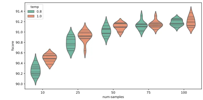
We now take a closer look at the approximate inference of the RNNG. The tempera-ture↵affects the proposal model and this, together with the number of samples, affects the approximate inference of the generative model. The temperature is used to flatten the proposal distribution to more evenly cover the support of the joint model, with the rationale of thus being closer to the true posterior;9 the number of samples is used to increase the accuracy of our unbiased MC estimate. The number of samples should particularly garner our attention: the approximate marginalization is compuationally expensive, requiring at least as many forward computations as there are unique sam-ples.10 The less samples we can get away with the better. To see how these values affect the generative RNNG in practice we perform two experiments: first we evaluate the RNNG with increasing number of samples, obtained with and without annealing; then we use these same samples to estimate the conditional entropy of the proposal models. For the first experiment we evaluate the generative RNNG as in the above setting, while varying the number of samples, and the temperature ↵: we let the number of
8The proposal samples used by Dyer et al. [2016] are availlable athttps://github.com/clab/rnng. 9After all, the proposal model was trained on a maximum likelihook objective, and we can thus expect it
to be too peaked.
10For efficiency we already partition the samples into groups of identical samples, where for each group
[image:35.595.118.479.188.247.2]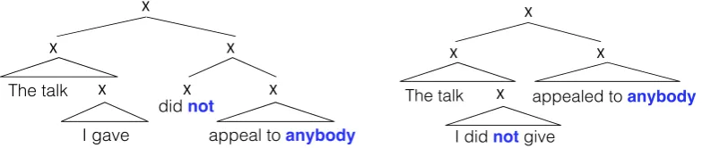
![Table 3.1.: Discriminative transition system. Example from Dyer et al. [2016].](https://thumb-us.123doks.com/thumbv2/123dok_us/8382387.320948/25.595.120.474.327.472/table-discriminative-transition-system-example-from-dyer-al.webp)
![Table 3.2.: Generative transition system. Example from Dyer et al. [2016].](https://thumb-us.123doks.com/thumbv2/123dok_us/8382387.320948/26.595.122.478.254.401/table-generative-transition-system-example-from-dyer-al.webp)