MoL 2017 24: Context Free Processes and Push Down Processes

Context-Free Processes and Push-Down Processes

MSc Thesis(Afstudeerscriptie) written by

Zeno de Hoop

(born August 17, 1991 in Goes, Netherlands)

under the supervision of Prof. Dr. Jos Baeten, and submitted to the Board of Examiners in partial fulfillment of the requirements for the degree

of

MSc in Logic

at the Universiteit van Amsterdam.

Date of the public defense: Members of the Thesis Committee:

Contents

1 Introduction 4

2 Preliminaries 6

2.1 Push-Down Automata . . . 6

2.2 Equivalences on PDA’s . . . 9

2.3 Process Specifications . . . 13

2.4 Greibach Normal Form for Sequential specifications . . . 19

2.5 PDA’s & Sequential Algebras . . . 22

3 Head-Recursion in Process Algebras 26

4 Transparency in Process Algebras 37

5 Combining Transparency and Head-Recursion 58

6 Transparency with Modified Process Algebras 67

Abstract

The purpose of this thesis is to examine in which cases context-free processes and push-down processes are the same. In particular, we de-part from the well-known case of language-equivalence and instead look at processes using process theory and more fine-grained equivalences, such as bisimulation and contrasimulation.

Acknowledgements

The first person I would like to extend my gratitude to is my supervisor, Jos Baeten, without whom the creation of this thesis would not have been possible. My interest in the topic of this thesis was sparked by his course ”Computability and Interaction”, and it was his enthusiastic teaching that made this one of the most memorable courses in my Master’s. He also encouraged us to try our hand at open problems in the field, which was the starting point of many of the ideas found in this thesis.

This brings me to two other people who deserve acknowledgement. The first is Sander in ’t Veld, a fellow student in the aforementioned course. It was one of his ideas, unpolished at the time, that eventually grew into one of the results found in this thesis (in particular, the result regarding head-recursion). This unpolished idea was then taken up by Fei Yang, who developed this idea further, bringing it very close to the final state found in this thesis. Finding a proof for this idea was one of the major breakthroughs in the process of writing this thesis, so I thank them both for their insight. I would further like to thank Fei Yang for having taken the time to proofread my thesis.

1

Introduction

The subject of this thesis is the relation between Context-Free Processes

and Push-Down Processes. However, since that statement is, in itself, too general to be useful, some further clarifications are in order.

To begin with, it is a well-known fact that for each context-free grammar one can find a push-down automaton that has the same language, and vice versa. This result can be found in many text-books on process or automata theory, among which [12].

However, with language-equivalence, one sees the behaviour of a system as merely the sequence of observable actions. This notion can be widened. One could for instance look at behaviour of a system as not only the total of events or actions that it can perform and the order in which they can be executed (as is the case with language-equivalence), but one could refine behaviour to include when certain ”decisions” are made. The latter is com-pletely abstracted from with language-equivalence: a process which decides its final action as soon as it begins, and one that only decides its final action at the very end are, under language-equivalence, indistinguishable.

With this in mind, we can make the method and purpose of this thesis a bit more precise. A process, in the context of this thesis, will be a la-belled transition system. This is a generalization of non-deterministic finite automata. This also means that we will only consider discrete processes.

The differences between processes, when given as labelled transition sys-tems, can be captured by equivalence relations on these systems. Language-equivalence is the most well-known of these Language-equivalences, but there are many more. Of particular interest to this thesis will be Bisimulation and Con-trasimulation. For more information on equivalence relations on transition systems in general, and a description of the lattice that these relations form, we refer to [8] and [7].

The primary question of this thesis will therefore be as follows: when is a process from a context-free grammar the same as a process from a push-down automaton? In particular, what is the finest equivalence relation realising this?

The structure of the thesis will be as follows:

• In the first section we present a number of definitions and relevant previous results.

• In the second section we give a proof of a conjecture from [14]; we show that for any sequential specification with head-recursion (with-out transparent names) one can construct a push-down automaton so that the associated transition systems are equivalent up to branching bisimulation.

we show that for any sequential specification with transparency (with-out head-recursion) one can construct a push-down automaton so that the associated transition systems are equivalent up to contrasimula-tion.

• In the fourth section we combine the results from the previous two sections: given a sequential specification, without restrictions on head-recursion or transparency, one can construct a push-down automaton so that the associated transition systems are equivalent up to con-trasimulation.

• Finally, in the fifth section, we show that, if one modifies one rule of the operational semantics, one can find the same result as detailed in the third section, but up to strong bisimilarity. We also briefly discuss the drawbacks of this rule change.

2

Preliminaries

This section covers a large part of the definitions used throughout the paper. The first subject covered is push-down automata, followed by equivalences on push-down automata, and finally process theory.

2.1 Push-Down Automata

As mentioned in the introduction, a push-down automaton is a transition system that goes from state to state by performing actions, and which has at its disposal a stack that may contain data. We will formally define the notion of a Push-Down Automaton that will be used in this paper. The definitions used in this section can be found in, for instance, [12].

Before detailing the definition of a push-down automaton, we will first define transition systems, as these will be routinely used throughout this work.

Definition 2.1. Let A be a set of actions, and A_τ = A ∪ {τ}, where τ is an unobservable action. A labelled transition system T is defined as a four-tuple (S,→,↑,↓) where:

• S is a (possibly infinite) set of states.

• →⊆ S × A_τ × S is a labelled transition. (s, a, t) is usually written as s−→a t.

• ↑∈ S is the initial state.

• ↓⊆ S is the set of terminating states.

We also introduce the following two bits of notation: with we mean the transitive-reflexive closure of−→τ , and→+_{indicates the transitive closure}

of−→τ .

We will now define what it means to be a push-down automaton. Infor-mally, a push-down automaton is a transition system which has access to a stack in which it can store data and later retrieve it.

Definition 2.2. APush-Down Automaton(PDA)M consists of a six-tuple (S,A,D,→,↑,↓) where:

• S is a finite set of states.

• A is a finite set of actions.

• D is a finite set of data.

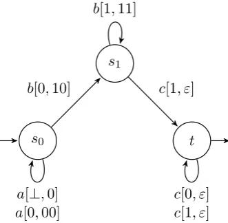
s0

s1

t b[0,10]

a[⊥,0] a[0,00]

b[1,11]

c[1, ε]

c[0, ε] c[1, ε]

Figure 1: example PDAM

• ↑∈ S is the initial state.

• ↓⊆ S is the collection of terminating states.

This definition needs some further clarification. ByA_τ is meant the set

A ∪ {τ}, whereτ is an unobservable action, not originally found inA, also referred to as silent or internal action. By D⊥ is meant the set D ∪ {⊥}, where⊥ is a special symbol indicating that the stack is empty. Finally, by

D∗ is meant a sequence of data symbols. As in [14], we often let δ and ζ range overD∗, and useεfor the empty string.

In terms of notation, if (s, a, d, δ, t) ∈→, we will write s −−−→a[d,δ] t. The meaning of this is as follows: if the PDA is at states, and the top element of the stack is d, then the PDA can perform action ato reach state t. The don top of the stack is replaced byδ. Note that aneed not be observable, and thatδcan be empty, that is,ε. A special case of note iss−−−→a[⊥,δ] t. This is an action that can be performed if the stack is empty.

Example 2.1. In figure 1, one can see an example of a PDA. In its initial state,s0, firstly,M can perform the action aan arbitrary number of times.

Each time a is performed, the symbol 0 is added to the stack. After the action a has been performed at least one time, M can perform the action b to go to state s1, which will add a 1 to the stack. At state s1, M can

perform the action b any number of times, and finally it can perform c to move to the statet. Attone can then performcas many times as there are items in the stack.

or not the stack starts empty, and whether or not one requires that the stack is empty before terminating, both influence the set of accepted strings.

Regarding the initial state of the stack, we will throughout this work assume that in a PDA’s initial state the stack is empty.

When it comes to the latter issue, there are three possible interpretations:

• FS (Final State): a PDA can terminate when it is in a final state

• ES (Empty Stack): a PDA can terminate whenever its stack is empty

• FSES (Final State Empty Stack): a PDA can terminate when its stack is empty, and it is in a final state.

So, looking at the previous example, we firstly see that under the FSES interpretation, the set of accepted strings is {a1+nb1+mc2+n+m|n, m ∈ _N}. This is almost the same as under the ES interpretation, except under the ES interpretation the empty string is also accepted. Finally, under the FS interpretation the accepted strings are {a1+nb1+mcp|n, m ∈ _N,0 ≤ p ≤

2 +n+m}.

In this work we will use the FSES interpretation (unless otherwise spec-ified). For further information on this topic we refer to [14].

Definition 2.3. Under a given interpretation, and given a PDAM, we call the setL(M)⊆ A∗ _{of all strings accepted byM thelanguage of M.}

Each PDA can also be transformed into a transition system.

Definition 2.4. Let M = (S,A,D,→,↑,↓) be a PDA. We then define the associated transition systemT(M) = (S_T(M),→_T(M),↑_T(M),↓_T(M)) as follows:

• S_T(M)=S × D∗_.

• The contents of the set→_T(M) are:

– (s, dζ) −→a (t, δζ) iff s−−−→a[d,δ] t for all s, t ∈ S, a∈ A, d∈ D, and δ, ζ ∈ D∗_.

– (s, ε)−→a (t, δ) iffs−−−→a[⊥,δ] t.

• The state (↑, ε) is the initial state ofT(M).

• The final states ofT(M) are↓T(M)={(s, δ)|s∈↓, δ∈ D∗}.

s2

s1

s3

s0

t4

t1

t0

t2

t5

b c

a

b c

a a

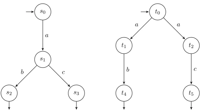
Figure 2: Two language-equivalent transition systems

Definition 2.5. Let M be a PDA which contains the states s, t ∈ S, and let a ∈ A, and d, e ∈ D. We call a transition a push-transition if it of the forms−−−→a[⊥,d] tors−−−−→a[d,ed] t. We call a transition apop-transition if it is of the form s−−−→a[d,ε] t.

2.2 Equivalences on PDA’s

In this subsection we will define the behavioural equivalences used in this work. The definitions are taken from [14], unless otherwise specified. Addi-tionally, for a more in-depth treatment of behavioural equivalences, we refer to [7].

Definition 2.6. Two PDA’s M andN arelanguage equivalent iff L(M) =

L(N). This is written as M ≈N.

Language equivalence is probably the most well-known, and most studied behavioural equivalence on automata. However, with language equivalence, a lot of information about the details of the process is lost. We will give an example of this in terms of transition systems.

Example 2.2. Consider the two transition systems given in figure 2. It should be clear that these two systems are language equivalent; they both accept the language {ab, ac}. However, their processes differ: in the left transition system one first makes ana-step, after which one chooses between b and c. In the system on the right one first chooses which a-step to take, after which one is forced to do aborc step, depending on one’s choice.

account the choice structure of the process. The behavioural equivalence that we will consider for most of the first part of this work is bisimulation.

Definition 2.7. LetT1 = (S1,→1,↑1,↓1) andT2 = (S2,→2,↑2,↓2) be

tran-sition systems. Abisimulation betweenT1 andT2 is an equivalence relation

R⊆ S₁× S₂ such that for alla,s1 ∈ S1 ands2 ∈ S2: • ↑1R ↑2.

• Ifs1Rs2 ands1

a

−

→s0₁ then there exists ans0₂ such that s2

a

− →s0₂.

• Ifs1Rs2 ands2 −→a s20then there exists ans01 such thats1 −→a s01. • Ifs1∈↓1 and s1Rs2 then s2 ∈↓2 and vice versa.

Transition systemsT1 and T2 are calledbisimilar if there exists a

bisimula-tion between them. The notabisimula-tion for this isT1-T2.

Revisiting the previous example, we can now see that while the two transition systems in figure 2 are language-equivalent, they are not bisimilar. This is becases0 would have to be related tot0 by virtue of being an initial

state, which would force one to relates1 to eithert1 ort2. However, there is

noc-transition fromt1, nor is there ab-transition fromt2, so no bisimulation

can be found.

The definition of bisimulation is sometimes also called strong bisimu-lation. As shown via the example, for strong bisimulation each transition needs to have an equivalent transition in the other transition system, in-cludingτ transitions. This requirement is too strong in some situations. We will therefore introduce the notion of branching bisimilarity.

Definition 2.8. LetT1 = (S1,→1,↑1,↓1) andT2 = (S2,→2,↑2,↓2) be

tran-sition systems. A branching bisimulation between T1 and T2 is a relation

R ⊆ S₁ × S₂ such that ↑₁ R ↑₂, and for all s1 ∈ S1 and s2 ∈ S2, s1Rs2

implies:

• ifs1

a

−

→s0₁ and a6=τ then there exists₂0, s00₂ ∈ S₂ such thats2s002

a

− →

s0₂, and both s1Rs200 and s01Rs02. • ifs1

τ

−→s0₁ then there exists0₂ ∈ S₂ such thats2s02, and s01Rs02.

• ifs2

a

−

→s0₂ and a6=τ then there exists₁0, s00₁ ∈ S1 such thats1s001

a

− →

s0₁, and both s00₁Rs2 and s01Rs02. • ifs2

τ

−→s0₂ then there exists0₁ ∈ S₁ such thats1s01, and s01Rs02. • ifs1∈↓1 then there exists as02∈ S2such thats2s02 and boths1Rs02

• ifs2∈↓2 then there exists as01∈ S1such thats1s01 and boths01Rs2

ands0₁ ∈↓1.

The transition systems T1 and T2 are branching bisimilar if there exists a

branching bisimulation between them. The notation for this isT1 -bT2. Finally, we might want our branching bisimulation to preserve diver-gences (that is, unbounded sequences of τ actions). This equivalence is called branching bisimilarity with explicit divergence in [7], but we will fol-low [14] in calling it divergence-preserving branching bisimilarity.

Definition 2.9. LetT1 = (S1,→1,↑1,↓1) andT2 = (S2,→2,↑2,↓2) be

tran-sition systems, and let R ⊆ S1× S2 be a branching bisimulation. This

re-lationR is a divergence-preserving branching bisimulation if for all s1 ∈ S1

and s2 ∈ S2,s1Rs2 implies:

• if there exists an infinite sequence (s1,i)i∈Nsuch thats1,0=s1,s1,j

τ

− →

s1,j+1, and s1,iRs2 for all i∈N, then there exists a state s02 such that

s2 →+ s02 and s1,iRs02 for somei >0.

• if there exists an infinite sequence (s2,i)i∈_N such thats2,0 =s2,s2,j τ

− →

s2,j+2, and s1Rs2,i for all i∈N, then there exists a state s01 such that

s1 →+ s01 and s01Rs2,i for somei >0.

The transition systemsT1 andT2aredivergence-preserving branching

bisim-ilar if there exists a divergence-preserving branching bisimulation between them. The notation for this isT1

-∆

b T2.

We note that branching bisimilarity and divergence-preserving branching bisimilarity have been proven to be equivalence relations on labelled transi-tion systems. For the proofs of this we refer to [6] and [10], respectively.

As mentioned at the end of the previous section, every PDA is, under a ”relevant equivalence”, equivalent to a PDA with only push- and pop-transitions. The relevant equivalence is divergence-preserving branching bisimulation, and we will prove this statement here, as it will make later results simpler to prove. This theorem can also be found in [14].

Theorem 2.1. For every PDA M there exists a PDA M’ which uses only push- and pop-transitions, such that T(M)

-∆

b T(M

0₎

Proof. We prove this by modifying any transitions inM that are not push-or pop-transitions.

• We constructM0 by modifying any transition of the types−−−→a[⊥,ε] tby adding an extra state s0 such thats

a[⊥,d] −−−→ s0

τ[d,ε]

• We modify any transition of the types−−−→a[⊥,δ] twhereδ =dn...d1 and

n≥2 by adding extra states s0, ..., sn−2 such that:

s−−−−→a[⊥,d1] s0

τ[d1,d2d1]

−−−−−−→...−−−−−−−−−−−→τ[dn−2,dn−1dn−2] sn−2

τ[dn−1,dndn−1]

−−−−−−−−−−→t

• Any transition of the types−−−→a[d/δ] twhereδ=d0d1..dn6=edfor some

ecan be modified to:

s−−−→a[d/ε] s0

τ[α/d0]

−−−−→s1

τ[d0,d1d0]

−−−−−−→...−−−−−−−−−−−→τ[dn−2,dn−1dn−2] sn−2

τ[dn−1,dndn−1]

−−−−−−−−−−→t

Hereα can be any single element from D ∪ {⊥}.

For every transition modified this way, it is clear that if we relate s∈M to s∈ M0, and t ∈ M to s0, ..., t ∈M0, we will have a divergence-preserving

branching bisimulation.

2.3 Process Specifications

In the previous section we have specified processes via automata. However, it is also possible to specify a process via a process specification, which corresponds to a grammar in language theory. In this section we will define a syntax and a semantics for this purpose. This section is largely based on the works of in [14] and [2] (the former, in turn, basing his work on [3] and [4]).

Definition 2.10. Given an alphabet A and a finite set N of names, a

Recursive Specification S is a set of equations that associates with every name inN a term, which is constructed as follows:

• 0 and 1 are terms.

• AnyN ∈ N is a term.

• For alla∈ Aand a term t,a.t is a term.

• For all termsx and y, the alternative compositionx+y is a term.

A recursive specification is interpreted as follows: to start with, 0 denotes a transition system with a single initial state, which is not final, and no transitions, and 1 a transition system with a single initial state, which is final, and no transitions.

Secondly, in the terma.N, the a. part is called the action prefix. So, if you haveN =a.M, this means that at N, one can perform an action ato reachM.

aand reachM, or one can performband terminate. We will refer to parts of an alternative composition as summands. So, in this example, a.M and b.1 are both summands of M.

We will now give the structural operating semantics for the previous definition. These semantics will allow us to reason what transitions will be possible in the labelled transition system that describes the context-free process of the recursive specification. These semantics were originally proposed by Plotkin in [13], and are also found in [2].

Definition 2.11. The Structural Operating Semantics (SOS) for recursive specifications is as follows. To begin with, ↓ denotes that a state is final, and−→a is ana-labelled transition. The following rules will define the precise semantics of these predicates.

For all terms P1, P10, P2, P20, we have the following:

1↓

In words: the term 1 always terminates.

a.P −→a P

This rule means that if a term has an action prefix, it can make a tran-sition of that type to that term.

P1

a

− →P₁0

P1+P2

a

− →P₁0

P2

a

− →P₂0

P1+P2

a

− →P₂0

The previous two rules say that and alternative composition can make ana-transition if and only if one of the summands can make ana-transition.

P1↓

(P1+P2)↓

P2↓

(P1+P2)↓

These two rules state that an alternative composition of terms can ter-minate if and only if one of the summands can terter-minate.

P1↓

N ↓

P1

a

− →P₁0

N −→a P₁0

These rules will be the basis for reasoning about transitions and steps of recursive specifications.

Definition 2.12. We call a recursive specification aLinear Specification if each term associated with a name is linear. A term islinear if it meets one of these two requirements:

• it is 0, 1, or of the forma.N, wherea∈ Aand N ∈ N • it is an alternative composition of two linear terms.

Using SOS, a term of a linear specification can also be associated with a (finite) automaton.

Definition 2.13. Given a linear specification and N ∈ N a term, we will callT(N) = (S,A,→,↑,↓) the finite automaton associated with this term, which we will be as follows:

• We let the set of statesS ⊆ N be those names reachable fromN.

• P −→a Q iffP =a.QorP contains a summanda.Q.

• N =↑

• P ∈↓ iffP = 1 or P contains a summand 1.

Note that here the choice of the N inT(N) determines what state will be the initial state, as linear specifications in themselves have no indication of a ”starting point”.

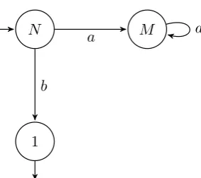
Example 2.3. Consider the following recursive specificationS:

N =a.M +b.1M =a.M

Now say that we’re interested in the associated labelled transition system

T_S(N). One could, for this, easily use the construction given in the previous definition, but by way of illustration we will piece it together here using the operational semantics.

To begin with, we have:

N M

1

a

b

a

Figure 3: The labelled transition systemT_S(N)

So therefore:

a.M+b.1−→b 1 Which means that we have:

N −→b 1 By the same reasoning, we therefore have:

N −→a M

And finally, since a.M −→a M, we also have:

M −→a M

We finally note that 1 is the only terminating term present. So putting all this together, we get the labelled transition system seen in figure 3.

Every linear specification therefore can therefore be associated with a finite automaton. The converse of this statement, moreover, is also true: given a finite automaton, we can find a linear specification that corresponds with it up to divergence-preserving branching bisimulation. This theorem can be found in [2].

Theorem 2.2. For every finite automatonM = (S,A_τ,→,↑,↓)there exists a linear specification with an initial nameI such that T(I)-M

Proof. We begin by associating with each state s ∈ S a name Ns, where

N↑ =I. The terms of each name will depend on the outgoing arrows of the state. The basic principle is, that for eachs−→a t, the term forNswill contain

a.Nt in its summation. Formally, we will define each name as follows:

Ns=

X

(s,a,t)∈→

The tail end of the term is a conditional addition, adding a 1 iff the state sterminates.

Using this construction, we can then easily verify that T(I) is stongly bisimilar toM.

To begin with, we will define the relation R as follows:

∀s∈ S.sRNs

We will now verify that R is indeed a strong bisimulation. We begin by noting that↑RN↑, so the initial states are related.

Secondly, ifs−→a tthen we havea.Ntas a summand ofNs, meaning that

we have Ns a

− →Nt.

For the third requirement we simply note that if Ns −→a Nt then a.Nt

must be a summand ofNs, and so we must have that s a

− →t.

Lastly, ifsterminates, then we have thatNs has as a summand 1, which

means thatNs terminates. The same holds in the opposite direction.

We therefore conclude thatR is a strong bisimulation, which concludes the proof.

We also note that every recursive specification

This shows that linear specifications are sufficient to describe finite au-tomata. However, since we also wish to look at algebraic specifications of PDA’s, we need to extend our algebra with another notion: sequential com-position.

Definition 2.14. Given an alphabet A and a finite set N of names, a

Sequential Specification S is a set of equations that associates with every name inN a term. These terms are recursively defined as follows:

• 0 and 1 are terms.

• AnyN ∈ N is a term.

• For alla∈ Aand N ∈ N,a.N is a term.

• For all termsx and y, the alternative compositionx+y is a term.

• For all termsx and y, the sequential compositionx·y is a term.

The sequential composition x·y means that one first performs x, and, whenx successfully terminates,y is performed.

We will now extend the SOS to include sequential composition.

P1 −→a P10

P1·P2 −→a P10·P2

In words, if one can make a transition, this transition will still be possible if another term is sequentially composed.

P1 ↓ P2 −→a P20

P1·P2 −→a P20

This rule states that, if, in a sequential composition, the first term can terminate, one can immediately start making transitions of the next term.

P1↓ P2 ↓

(P1·P2)↓

This rule states that if two terms terminate, then the sequential compo-sition of these terms terminates as well.

We will now introduce the notion of sequential term, the primary func-tion of which is that it makes sequential specificafunc-tions easier to read.

Definition 2.16. A Sequential Term is a term that only contains 0, 1, action prefixes, names, and sequential composition (that is, anything but alternative composition). We say that a specification is in Sequential Form

if each name is associated with an alternative composition of sequential terms.

Lemma 2.1. Each sequential specification is strongly bisimilar to a sequen-tial specification in sequensequen-tial form.

Proof. We will specify how to transform a specification that is not in se-quential form. The only way that a specification could be not in sese-quential form is if there exists a namen∈ N that contains a summand that is not a sequential term. For a term to be not sequential, it must contain alternative composition. This means that N must contain a summand that can be in one of the following three shapes: α·(β+γ), (β+γ)·δ, or α·(β+γ)·δ, whereα, β, γ, δ are terms.

For the sake of brevity we will only consider the third case, as the pro-cedure for the previous two can be easily deduced from it. The idea is that we simply introduce a new nameN0, such thatN0 =β+γ, and we rewrite the non-sequential term ofN asα·N0·δ.

It is additionally possible to rewrite any sequential specification in such a way that each summand contains at most two sequentially composed names.

Lemma 2.2. Given a sequential specification S and a name X in S, it is possible to find a sequential specification S0 such that all summands in all names inS0 contain at most two sequentially composed names, andT_S(X)

-T_S0(X).

Proof. This is a relatively simple matter of rewriting. Let S consist of the names Xi, where i = 0,1, ..., n. We then introduce new names Yij, where

Yij =XiXj. One can then replace, in any sequential composition, starting

from the left, a set of two names by their joint name. This process can then be repeated until all sequential compositions of names are of length 2 or less.

Finally, we will define what we mean by a head-recursive term, as this will be relevant in later sections, and it is a central notion in one of the new results presented in this paper.

Definition 2.17. We call a termN Head-Recursive if its alternative compo-sition contains a term of the formN·X, whereX is a non-empty sequential composition of names.

2.4 Greibach Normal Form for Sequential specifications In this section we will detail the Greibach Normal Form (GNF) for sequen-tial specifications, which was introduced in [11]. This specific form for se-quential specifications will be used for many results, not least of which the language equivalence between PDA’s and sequential specifications in GNF, to be detailed in the next section.

We begin by defining when a term is considered guarded as a basic notion that will be extended to pre-GNF, which will finally be developed into GNF proper.

Definition 2.18. A term in a sequential specification S is guarded if it is of the forma.X, wherea∈ Aτ, and whereX is a sequential composition of

one or more names, or 1.

Note that this means that, for instance, terms of the form a.0 are not considered guarded.

Definition 2.19. A sequential specification S is in pre-Greibach Normal Form (pre-GNF) if every term associated with a name N meets one of the following requirements:

• It is an alternative composition of one or more terms. Each of these terms is of one of the following forms:

– The term is guarded.

– The term is 1.

– The term is of the formN ·X, whereN is head-recursive.

Theorem 2.3. Given a sequential specification S, there exists a sequential specificationS0 such that S0 is in pre-GNF, and S-S

0_.

Proof. We will detail how to obtainS0 by rewritingS in bisimilar ways. To begin with, one rewrites S to be in sequential form (see previous section). Any single variables can then be replaced by the term associated with their names, or, if they are of the shape N =N +x, then the single variable N inN can be removed entirely (since N -x).

If any alternative composition contains the termN·X, whereX is non-empty, then this can be rewritten by replacing N with its associated term inS. If one encounters a name N that has N ·X as a summand, then this summand is head-recursive and can be left as is.

Pre-GNF is designed to preserve bisimilarity. If one is merely concerned with language equivalence, then one can use GNF proper:

Definition 2.20. A sequential specification S is inGreibach Normal Form

(GNF) if every term associated with a name meets one of the following requirements:

• The term is 0

• It is of the formP

a.X(+1), where a∈ A ∨a=τ,X is a sequential composition, and (+1) means that it has an optional 1-summand.

Theorem 2.4. For every sequential specification S there exists a sequential specificationS0 such that S0 is in GNF and S≈S0

Proof. Firstly, we rewriteS intoS00, whereS00 is in pre-GNF, andS

-∆

b S

00

(and therefore S ≈ S00). We can then simply rewrite any head-recursive terms N ·X into τ.N·X, which will give S0 in such a way that S00 ≈ S0, and so by transitivity of language equivalence, we get S≈S0.

Now, if we look at transition systems associated with sequential specifi-cations in GNF, we see a desirable property emerge, namely, that no infinite or unbounded branching occurs. Additionally, it will contain only one final state.

Theorem 2.5. If S is a sequential specification in GNF, and no names in

S contain a 1-summand, thenTS(I), where I is a name occurring inS, will

Proof. Firstly, the states of the transition system will be labelled by the names in S, all sequential compositions of names reachable from S, and finally of a state labelled 1. The state labelled 1 will be the only terminat-ing state, as no terms associated with names have immediate termination. Additionally, as may be clear, the state labelledI will be the initial state.

Now, for every state X, whereX is a non-empty composition of names, all the outgoing transitions will be dependent on the first name in the se-quential composition ofX. For example, say thatX=N·Y andN contains the summanda.Z, then in the transition system one will have X −→a Z ·Y. This means that every state will have at most as many outgoing arrows as there are summands in the first name of the sequential composition. Since this is by definition finite, this means that all branching in TS(I) will be

finite, and therefore bounded.

We will now also define what it means to be a sequential language, and what it means to be a sequential process.

Definition 2.21. Given a sequential specification S and an initial nameI, we will denote the language associated with this specification asL_S(I).

Definition 2.22. Given a sequential specification S and an initial nameI, theSequential Process PS(I) is the divergence-preserving branching

bisimi-larity class of transition systems that contains the transition system TS(I).

Theorem 2.6. The class of sequential processes is closed under + and ·. Proof. LetP_S(I) andP_T(J) be sequential processes, and letS∩T =∅.

• P_S(I) +P_T(J) =P_S∪T(I+J).

• PS(I)· PT(J) =PS∪T(I·J).

Theorem 2.7. The class of sequential languages is closed under union and concatenation.

Proof. Let LS(I) and LT(J) be sequential languages, and let S∩T = ∅.

The proof is then identical to the proof above, except regarding language rather than processes.

Theorem 2.8. Sequential languages (and therefore by extension sequential processes) are not closed under intersection and taking the complement.

Proof. This is proven by counterexample. Consider the following two se-quential specifications:

T ={J =K·L, K = 1 +a.K, L= 1 +b.L·c.1}

Given these specifications, we know that L_S(I) = {anbncm|n, m ≥ 0}

and LT(J) = {anbmcm|n, m ≥ 0}. However, this means that LS(I) ∩

L_T(J) ={anbncn|n≥0}, which is well known to be non-sequential [1]. This result also immediately gives us the fact that sequential languages are not closed under taking complement. Consider the following set-theoretic fact:

(UC ∪VC)C =U ∩V

Therefore, if sequential languages were closed under taking complement, they would be closed under intersection as well, which is a contradiction.

2.5 PDA’s & Sequential Algebras

This section will contain a number of results pertaining to the link between push-down automata and sequential specifications. The following proof is based mostly on [14], and has been slightly modified to suit the purpose of this work.

Theorem 2.9. Given a sequential specification Ein Greibach normal form, where E contains no transparent names, and an expression Px from this

specification, there exists a Push-Down Automaton (PDA) M (under the FSES interpretation) consisting of one state such that TE(Px)

-∆

b T(M),

on the condition that M may start with a non-empty stack.

Corollary 2.1. Given a sequential specificationE in Greibach normal form, and an name Px from this specification, there exists a Push-Down

Automa-ton (PDA)M (under the FSES interpretation) consisting of two states such thatTE(Px)

-∆

b T(M).

Proof. Let E = {Pi = P j∈Ji

aij.ξij|i ∈ I} be a sequential specification in

Greibach normal form (GNF), andx ∈I. Here ξj is a finite list of

sequen-tially composed names from E.

The claim is now that this sequential specification can be simulated by a one-state PDA. This PDA is constructed as follows:

• One state, N, whereN ↑ andN ↓.

• For alli∈I, letN −−−−−→aj[Pi/ξj] N for all j∈J.

The claim is thatT_E(Px)

-∆

b T(M). Firstly, forTE(Px) the construction

detailed previously is used. Note in particular that this means that for a state Piχk, (where χk is either empty or a list of names from E) it holds

thatPiχk aj

−→ξjχk iff Pi containsajξj as part of its alternate composition.

Secondly, forT(M) the standard construction given earlier is used. This means that in the transition system, for any state (N, sζ) (where sζ is a stack with the element s on top) we have (N, sζ) −→at (N, ρζ) iff in M we haveN −−−−→at[s/ρ] N.

Now, to prove thatT_E(Px)

-∆

b T(M), letR ⊆S×T, whereS is the set

of states from T_E(Px) and T is the set of states from T(M). We define R

as follows: simply letαR(N, α), where α is a list of names from E.

Now all that is left is to show that this is a branching bisimulation that preserves divergencies. First, we show that it is a bisimulation. For this, let αi =Pyβi and αiR(N, αi).

Now, for the first condition of bisimulation, ifαi −→az αj, this means that

αj = ξzβi, and that, in E, the alternate composition of Py contains az.ξz.

This then implies that in the PDA M we haveN −−−−−−→az[Py/ξz] N, which implies that in T(M) we have (N, Pyβi)

az

−→(N, ξzβi), which proves the condition.

Since the reverse of all these implications also holds, this also proves the second part of the definition. Furthermore, we note that this reasoning also holds for the terminating states, proving that R is in fact a bisimulation. Not only does it prove this, but it also shows thatTE(Px) andT(M) are in

fact isomorphic.

For the corollary one only needs to add one extra state Q to M, which will be the initial state instead of N, and the transitionQ−−−−−→τ[⊥/Px] N. It is then easy to show that the previous result still holds, although only up to divergence preserving branching bisimulation.

Corollary 2.2. Under the FS interpretation of PDAs, one additional state is needed.

Proof. Under the FS interpretation one will need to add an additional state N0, which will be the only terminating state (meaning thatN will no longer terminate), and the transition N −−−−→τ[⊥/ε] N0. It can easily be checked that this PDA is still branching bisimilar with divergencies to E.

This result can also be used to get another classic result pretty much immediately:

Theorem 2.10. Given a sequential specification S and an initial name I, there exists a PDA M such that L_S(I)≈ L(M).

One can also prove the converse (adapted from [12]).

Theorem 2.11. Given a PDA M, there exists a sequential specification S

with an initial stateI such that S is in GNF, and L(M)≈ L_S(I).

Proof. Firstly, under language equivalence we can safely assume the follow-ing thfollow-ings aboutM:

• M has only one final state.

• M has only push/pop transitions.

The sequential specificationS will now be constructed as follows: firstly, one creates namesV_s∅ andVsdt for alls, t∈ S andd∈ D. These names then

get assigned summands as follows:

• We assign to V_s∅ the summanda.Vtdu·Vu∅ for everyu∈ S and every steps−−−→a[∅/d] t.

• We assign toVsdt the summand a.1 for every steps a[d/ε] −−−→t.

• We assign to Vsdt the summand a.Vuev ·Vvdt for every t, v ∈ S and

every step s−−−−→a[d/ed] u.

• We assign toV↓∅ the summand 1.

Any names without summands will be assigned the constant 0.

The basic idea of this construction is as follows: basically, the names will encode both the contents of the stack, and, so to say, a potential order in which the content of the stack will be ”spent”. So, say that we are in Vs∅, and there is a steps−−−→a[∅/d] t. This means that the alternate composition of V_s∅ will most likely contain many summands of the form a.Vtdu·Vu∅. Note that for eachVtdu there are two options: either thedin the stack is ”spent”

in the step to u, in which case it can terminate by choosing the summand a1, after which the process will be at the name V_u∅, or another element is gained, in which case the list of sequentially composed names increases (and so do the potential options).

It is therefore clear that if the PDAM accepts a certain word, then the sequential specificationS will too. However, one could still worry that, since so many potential (and potentially impossible) paths are created, perhaps S will accept more than M. However, it is not hard to see that this will never happen: say that one chooses a summand with an impossible path. Firstly, we can assume that the final name in the sequential composition is V↓∅, as otherwise the state will not terminate. Secondly, we can assume that all names of the shapeVsdt will no longer choose any summands of the form

Given these assumptions, it must then mean that there is a Vsdt such that

no step of the form s −−−→a[∅/d] t exists. However, this means that Vsdt = 0,

X

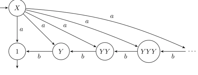
1 Y Y Y Y Y Y · · ·

a a a

a a

b b b b

Figure 4: Transition systemT_S(X)

3

Head-Recursion in Process Algebras

We have seen that, given a sequential specification in GNF, one can find a PDA such that the respective transition systems are divergence-preserving branching bisimilar. In this section we will look at sequential specifications containing head-recursion.

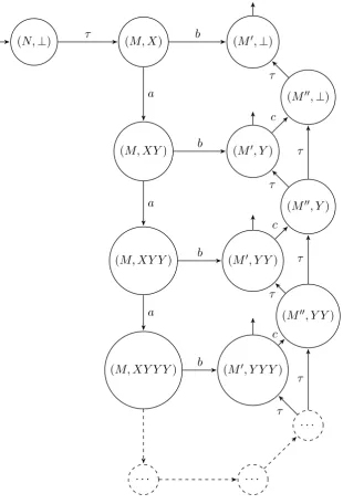
Example 3.1. Consider the following sequential specification S:

X=X·Y +a.1 Y =b.1

If we expand the equation for X we see that the following transitions will be possible:

X −→a 1 X·Y −→a Y

X −→a Y

X·Y −→a Y ·Y

X −→a Y ·Y

X·Y −→a Y ·Y ·Y

X −→a Y ·Y ·Y

And so on. It is clear that one can therefore, fromX, make ana-step to an infinite number of states. The transition-system T_S(X) is therefore like in figure 4.

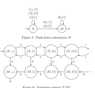
N M τ[⊥/1]

τ[1/11] τ[1/ε]

a[⊥/ε] a[1/1]

b[1/ε]

Figure 5: Push-down automatonM

(N,⊥)

(M,⊥) (M,1) (M,11) (M,111) · · ·

(N,1) (N,11) (N,111) · · ·

a τ

b b b b

τ

a τ

τ

a τ

τ

a

τ

τ

Figure 6: Transition systemT(M)

from the branching bisimilarity, it is possible. Consider the PDA shown in figure 5, and the associated transition system seen in figure 6.

We will now show thatT_S(X) andT(M) are branching bisimilar. Con-sider the following relationR:

R={(X,(N,1n))|n= 0,1, ...} ∪ {(Ym,(M,1m))|m= 0,1, ...}

One can easily verify thatRis a branching bisimulation. The main point of the proof is that, since all (N,1n) are related to X, the newly introduced τ-transitions simply correspond to standing still in T_S(X). Additionally, since one can move along the string of (N,1n) states freely, any step from X toYm can be simulated by (N,1n)(N,1m)−→a (M,1m).

The previous example illustrates the basic idea of the more general case: to deal with recursion, one ”unravels” the state in which the head-recursion occurs to form a string of states where one can get to any state us-ing onlyτ-transitions (introducing divergencies where they previously didn’t exist, meaning that it only works up to branching bisimilarity).

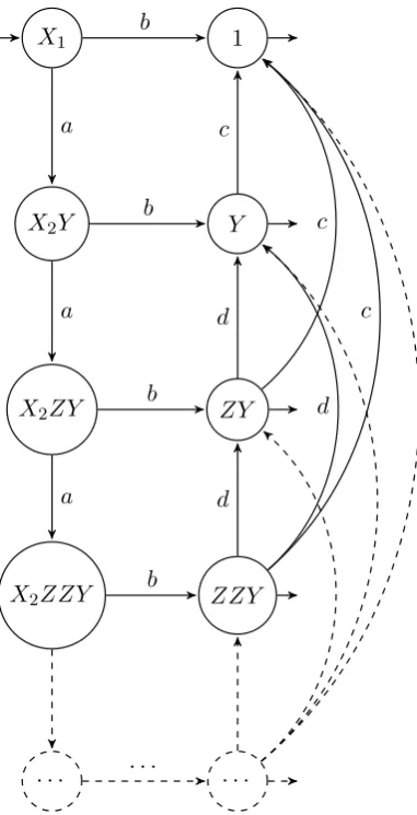
However, when one tries to generalize this idea, one runs into additional problems, illustrated by the next example:

X=X·Y +a.1 +c.Z Y =b.1

Z =d.X

When figuring out the transition systemT_S(X), we begin by noting that the steps derived in example 3.1 are still possible. That is, there still exists the transition X −→a Yn for any n ∈ _N. However, when expanding the equations, an additional pattern starts to emerge:

X −→c Z

X·Y −→c Z·Y

X −→c Z·Y

X·Y −→c Z·Y ·Y

X −→c Z·Y ·Y

X·Y −→c Z·Y ·Y ·Y

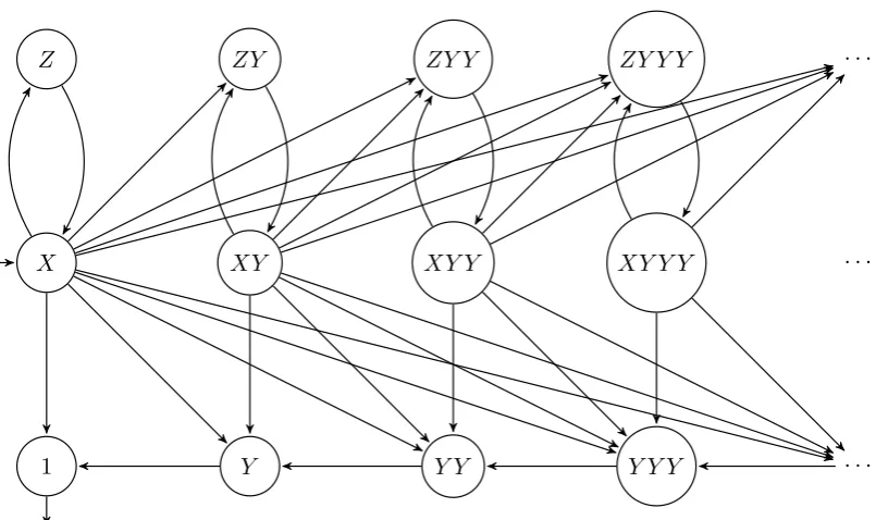
So the transition X−→c ZY is possible, from where one is forced into the transition ZY −→d XY. So, contrary to Example 3.1, hereXY (and XY Y, and XY Y Y, etc.) are proper states. These states are clearly not identical toX, as one cannot transition from XY Y straight toY, for instance. The transition systemTS(X) can be seen in Figure 7 (for the sake of readability

the transitions have been left unlabelled, but the action associated with the transition should in all cases be clear).

Keeping this difficulty in mind, we will now treat the more general case, where only the initial state is head-recursive.

Theorem 3.1. Let S be a sequential specification defined by a set of vari-ables {X, Yi|i= 0,1, ..., n} as follows:

X=X·Y0+

X

k∈IX

ak.ξk

Yi=

X

j∈Ii

aij.ξij

Hereξ is a sequential composition of any number of variables, where zero variables is understood to be equal to1.

X

1 Y Y Y Y Y Y · · ·

XY XY Y XY Y Y · · ·

Z ZY ZY Y ZY Y Y · · ·

Figure 7: Transition system of a more complex head recursion

Proof. Keeping the difficulties from the previous example in mind, we in-troduce the segment symbol , with which we will mark any return to the head-recursive stateX, so that we don’t accidentally throw away any previ-ously committedY0’s from the stack. The set of data Dused by this PDA

will therefore be defined as {X, Yi|i = 0,1, ..., n} ∪ {}. The PDA P will

consist of three states, {1, N, M}. The state 1 will simply behave as the terminating state. The state N will take care of the head-recursion of X, and will therefore behave as follows:

N −−−−−→τ[⊥/Y0] N

N −τ−−−−−−[Y0/Y0Y0→] N

N −−−−→τ[Y0/ε] N

N −−−−−→τ[/Y0] N

∀k∈IX, d∈ D.N

ak[d/ξkd]

−−−−−−→M

The first four steps take care of the head-recursion: it allows the PDA to stack and remove as manyY0’s as is needed, though anyY0’s on the stack

terminate at this state, and the final scheme for steps indicate that at any pointN can choose any other summand.

The second state,M, will simulate the behaviour of all other variables:

∀i∈ {0,1, ..., n}, j ∈Ii.M

aij[Yi/ξij]

−−−−−−→M

M −−−−→τ[⊥/ε] 1 M −−−→τ[/ε] M

M −−−−→τ[X/] N

The first two lines specify the simulation of the Yi variables, functioning

in the same vein as before. The latter two lines specify the functioning of the segment symbol.

This concludes the specification of the PDA P. All that remains is to show that TS(X) -∆ T(P). For that we will first introduce some new notation, to enhance readability.

Firstly, we will denote with ζ a string of variables fromS, possibly also containing the segment symbol . To put it more formally, ζ ∈(S∪ {})∗ Withζ−we will mean the stringζ, but with any segment symbols removed. With ζ is meant any element from the set of strings that one can obtain by placing segment symbols anywhere in the string ζ. Finally, with the notation []ζ we mean the stringζ ifζ is not empty, and the empty string otherwise.

We will now give the relationR⊆ T_S(X)×T(P) that will be our branch-ing bisimulation:

∀ζ ∈S∗.ζ R(M, ζ)

∀m∈_N.X R(N, Y₀m)

∀ζ ∈S∗.Xζ R(N, Y₀mζ))

1 R1

Wherem∈N.

To prove thatRis a branching bisimulation, we first check that↑1 R↑2.

Since↑₁=X, and↑₂= (N,⊥), andXR(N,⊥), this first condition is satisfied. For the rest of the conditions, assume thats1Rs2.

• If s1 −→a s01 and a =6 τ, we claim that there exist s02, s002 ∈ T(P) such

thats2s002

a

−

→s0₂ ands0₁Rs0₂.

First, assume that s1 = Xζ, with ζ potentially empty. Then s2 =

(N, Ym[]ζ), or s2 = (M, Xζ). However, the latter reduces to the

non-τ steps from s1, namely that s01 = ξkYm

0

0 ζ, so the step taken is

Xζ −→ak ξkYm

0

0 ζ, or, in words, one goes down the head-recursion m0

times, and then chooses another, non-head-recursive summand from X. Then the desired states in T(P) are s00₂ = (N, Y₀m0[]ζ) and s0₂ = (M, ξkYm

0

0 []ζ). This is because

(N, Y₀m[]ζ)(N, Y₀m0[]ζ)

since one can freely change the number ofY0’s on the stack in the state

N, and since∀k∈IX, d∈ D.N

ak[d/ξkd]

−−−−−−→M, we have:

(N, Y₀m0[]ζ)−→ak (M, ξkYm

0

0 []ζ)

Additionally, it is easy to see that these states also relate in the correct way:

XζR(N, Y₀m0[]ζ) ξkYm

0

0 ζR(M, ξkYm

0

0 []ζ)

meaning that the requirements for branching bisimilarity are, in this case, satisfied.

So if s1 = Xζ, this requirement for bisimilarity holds. We will now

consider the simpler case where s1 = Yiζ. This means that s2 =

(M, Yiζ). The only possible transition in this scenario is a transition

wheres0₁ =ξijζ and so the transition made isYiζ aij

−−→ ξijζ. However,

since this means that Yi contains the summand aij.ξij, we also have

thatM −−−−−−→aij[Yi/ξij] M, and so we have:

(M, Yiζ) aij

−−→(M, ξijζ)

And additionally we know that:

ξijζR(M, ξijζ)

Therefore, for every non-τ transition from s1 we can find the

appro-priates00₂, s0₂ to satisfy branching bisimilarity.

• If s1

τ

−

→ s0₁, then there exists a s0₂ such that s2 s02 and s01Rs02. If

there is a transition from s1 of the shape s1

τ

−

→ s0₁, then this means that the first variable in the name of s1, say Zi, must have contained

a summand of the shape τ.ξij, which means that the proof for the

• If s2

a

−

→ s0₂ and a 6= τ, then there exist s0₁, s00₁ ∈ T_S(X) such that s1 s001

a

− →s0₁.

First, we look at the case wheres2 = (N, Y0m[]ζ). This means thats1

must be the stateXζ−. There is now only one non-τ transition that can be made froms2, and that is the case in whichs02 = (M, ξkYm[]ζ),

so the transition made is:

(N, Y₀m[]ζ)−→ak (M, ξkYm[]ζ)

Here we have that s00₁ = s1 and s01 = ξkYmζ−. Since the transition

in T(M) is possible because X contains the summand ak.ξk, we can

similarly inT_S(X) make the transition:

Xζ−_−→ak

ξkYmζ−

And we know that:

ξkYmζ−R(M, ξkYm[]ζ)

So ifs2 = (N, Y0m[]ζ), this requirement of bisimilarity holds.

The only other option is that s2 = (M, Yiζ). Note that we do not

consider the state (M, Xζ) and (M,⊥) here: this is because no non-τ steps can be taken from these states.

Ifs2 = (M, Yiζ), we know that s1 =Yiζ−. All non-τ transitions that

can be taken froms2 are of the following shape:

(M, Yiζ) aij

−−→(M, ξijζ)

Again, if this transition is possible, it must be that inM we have the transitionM −−−−−−→aij[Yi/ξij]. If this step exists inM, then we know thatYi

must haveaij.ξij as a summand. Which in turn means that inTS(X)

we can make the following transition:

Yiζ− aij

−−→ξijζ−

Which is, of course, the desired transition, since:

ξijζ−R(M, ξijζ)

Which means that, in every scenario, ifs2

a

• If s2

τ

−

→ s0₂, then there exists a s0₁ ∈ T_S(X) such that s1 s01 and

s0₁Rs0₂.

This direction of the requirement onτ steps requires a bit more work than its converse, since T(M) contains many more silent transitions than its process-algebraic counterpart.

First, we consider the case in which s2 = (N, Y0m[]ζ). This means

thats1 =Xζ−. In this case, only one type of silent transition can be

made: M can either add, or remove, aY0 from the stack. So:

(N, Y₀m[]ζ)→−τ (N, Y₀m±1[]ζ)

In this case, one simply takess0₁ to be equal tos1, sinces1 s01 is not

only the transitive, but also reflexive closure ofτ, and additionally we have

Xζ−R(N, Y₀m±1[]ζ) Meaning that for this case, the requirements hold.

The second scenario we will consider is s2 = (M,⊥). Here it must

be the case that s1 = 1. The only possible transition from s2 is

(M,⊥)−→τ 1, which poses no problems since 1R1.

The third scenario to consider is when s2 = (M,ζ). Here we must

haves1 = (ζ)−=ζ−. The only possibility fors02 here iss02 = (M, ζ),

as no otherτ-transitions exist from this state but the following one:

(M,ζ)−→τ (M, ζ)

However, again, this is no problem, as we can simply chooses0₁ =s1

once more, as ζ−R(M, ζ).

Finally, the fourth case to consider is when s2 = (M, Xζ). Here we

have thats1 =Xζ−, and the only possible option fors20 iss02= (N,ζ),

so the transition is:

(M, Xζ)−→τ (N,ζ)

Which, like before, is no issue if one takess0₁=s1, as Xζ−R(N,ζ).

As a final note, anyτ-transitions not covered by these cases are tran-sitions based on summands in S, which means that the proof in the previous bullet-point applies.

• If s1 ∈↓1, then s1 = 1, and so it must be the case that s2 = 1, and

therefore s2 ∈↓2, as 1R1. The converse also holds, as both transition

This concludes the proof of R being a branching bisimilarity.

With this, we can make a further generalization to cover all non-transparent, head-recursive sequential specifications.

Theorem 3.2. Let S be a sequential specification defined by a set of vari-ables {Xi, Yi0|i= 0,1, ...n∧i0= 0,1, ..., n0} as follows:

Xi =

X

j∈Ii

Xi·Vij +

X

k∈Ji

aik.ξik

Yi0 =

X

j0_∈I i0

ai0_j0.ξ_i0_j0

Let Z and eachVij be a name from S. There exists a PDAP such that

TS(Z)-∆T(P).

Proof. The PDA P will follow the same principles as the PDA seen in the previous proof. The two main differences, in words, will be the following: to begin, each Xi, that is, each head-recursive name, will get its state, Ni,

which can add or remove anyVij at will. The second difference is that each

Xi is now allowed to contain any finite number of head-recursive summands.

This does not change anything fundamentally: it simply means that one can jump to any sequence ofVij’s fromX.

The basic part of the PDA will therefore look as follows:

∀i= 0,1, ..., n;j∈Ii.Ni

τ[⊥/Vij]

−−−−−→Ni

Ni

τ[Vij/VijVij]

−−−−−−−−→Ni

Ni

τ[Vij/ε]

−−−−−→Ni0

Ni

τ[/Vij]

−−−−−→Ni

∀k∈Ji, d∈ D.Ni

aik[d/ξikd]

−−−−−−→M

∀i0 ∈ {0,1, ..., n0}, j0 ∈Ii0.M

a_i0_j0[Y_i0/ξ_i0_j0]

−−−−−−−−→M

M −−−−→τ[⊥/ε] 1 M −−−→τ[/ε] M

M −−−−→τ[Xi/] Ni

M0−−−−→τ[⊥/Z] M

The relationR⊆ T_S(Z)× T(P) that will be our branching bisimulation will also not hold any particular surprises:

ζR(M, ζ) ZR(M0,⊥) Xiζ1R(Ni, ζ2ζ

1)

Xiζ1R(Ni0, ζ2ζ1)

1R1

As for the proof, all the work is essentially done in the preceding proof: for each moment of head-recursion inS, the stateM sends one to the appro-priate stateNi, where the desired stack can be freely generated, before being

sent back to M to proceed. The only thing left to check is the transition from the newly made stateM0:

(M0,⊥)−−−−→τ[⊥/Z] (M, Z)

4

Transparency in Process Algebras

In this section we will look at sequential specifications that contain transpar-ent names, and show that these specifications can be emulated by push-down automata up to contrasimulation.

We will begin by defining contrasimulation. Recall that with we mean the transitive, reflexive closure ofτ-transitions. We also introduce the following new notation: with s−→a→twe mean su−→a vt.

Definition 4.1. LetT1,T2be labelled transition systems. A pair of relations

(R, Q), whereR⊆ T₁× T₂ and Q⊆ T₂× T₁ is a contrasimulationif it meets the following requirements.

First, we have that ↑1 R↑2 and↑2Q↑1.

Lets1Rs2. Then: • If s1

a

−

→→ s0₁ and a 6= τ, there exist s0₂ ∈ T₂ such that s2

a

−

→→ s0₂, and s0₂Qs0₁.

• Ifs1

τ

−→→s0₁, then there exists a s0₂∈ T₂ such that s2 s02 and s02Qs01. • If s1 ∈↓1, then there exists as02 ∈ T2 such that s2 s02, s02 ∈↓2 and

s0₂Qs1.

Secondly, we require the converse of the above requirements to hold: Lets2Qs1. Then:

• If s2

a

−

→→ s0₂ and a 6= τ, there exist s0₁ ∈ T₁ such that s1

a

−

→→ s0₁, and s0₁Rs0₂.

• Ifs2−→τ→s02, then there exists a s01∈ T1 such that s1 s01 and s01Rs02. • If s2 ∈↓2, then there exists as01 ∈ T1 such that s1 s01, s01 ∈↓1 and

s0₁Rs2.

We note that contrasimulation sits between _-b and ≈ in Glabbeek’s

lattice of equivalences. For more details we again refer to [7].

Before we present any general results, we will first consider a number of examples. The first example is the ”canonical” example of why transparency in process algebras can be troublesome.

Example 4.1. Consider the following specification S:

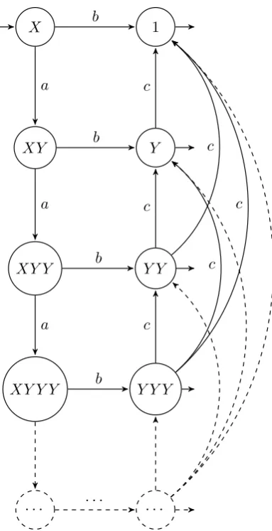
X=a.X·Y +b.1 Y =c.1 + 1

In figure 8 one can see the transition system TS(X). It is clear that

X 1

Y

Y Y

Y Y Y

· · ·

XY

XY Y

XY Y Y

· · ·

b

a c

c

c

c

c c a

b

a

b

b

· · ·

Figure 8: Transition systemTS(X)

contains the summand 1, this means that it is possible to make the transi-tion Yn −→c Ym for any m < n, and since one can also choose to pick the 1-summand in allY’s, we have that allYn states terminate.

Now, where the previous results worked for the FSES interpretation of PDA’s, here we are forced to limit ourselves to FS. This is to be able to deal with the fact that arbitrarily large sequences of names can instantaneously terminate (provided that all names are transparent).

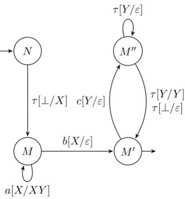
Now, our goal with this example is to find a PDA that will be equivalent toT_S(X) up to contrasimulation. We claim that the PDAP, shown in figure 9 will do exactly that. The associated transition system T(P) is shown in figure 10.

M M0 M00 N

τ[⊥/X]

a[X/XY]

b[X/ε]

c[Y /ε] τ[Y /Y] τ[⊥/ε] τ[Y /ε]

Figure 9: Push-down automaton P

transparency in the context of contrasimulation, so it will be informative to look at the contrasimulation (R, Q) in detail.

To begin with, we will defineR as follows:

X R(N,⊥)

∀n∈_N.XYn R(M, XYn)

∀n∈N.Yn R(M0, Yn)

∀n∈N.Yn R(M00, Yn)

And we will define the relation Qas follows:

(N,⊥) QX

∀n∈_N.(M, XYn) QXYn

∀n∈N.(M0, Yn) QYn

Note that none of the states originating from M00 have a relation in the Q-direction.

Now, we want to show that this is indeed a contrasimulation. We be-gin by noting that XR(N,⊥) and (N,⊥)QX, meaning that we meet the requirement that the initial states should be related in both directions.

(M, X) (M0,⊥)

(M0, Y)

(M0, Y Y)

(M0, Y Y Y)

· · ·

(M, XY)

(M, XY Y)

(M, XY Y Y)

· · ·

(M00,⊥)

(M00, Y)

(M00, Y Y)

· · ·

(N,⊥) b

a

c

c

c a

b

a

b

b

τ

τ τ

τ τ

τ τ τ

• If s1

a

−

→→ s0₁ and a 6= τ, there exist s0₂ ∈ T₂ such that s2

a

−

→→ s0₂, and s0₂Qs0₁.

Ifs1 =XYn for anyn∈N, we must haves2 = (M, XYn). Then the

only options are to take anaor a b transition. The former transition will be:

XYn a−→XYn+1

Which can be mirrored inT(P) by:

(M, XYn)−→a (M, XYn+1)

And we have that (M, XYn+1)QXYn+1. Identical reasoning applies for theb-transition.

The more interesting case is whens1=Yn. We have two options here

fors2, but we begin by considering the case wheres2 = (M00, Yn) (the

other option, where s2 = (M0, Yn), will also be covered by this case).

We can then make the following transitions:

∀m < n.Yn c−→Ym

Now, we can mirror this as follows:

(M00, Yn)−→τ (M0, Yn)→−c (M00, Yn−1)(M0, Ym)

And since (M0, Ym)QYm, the requirement is met.

• The requirement aboutτ-transitions need not be considered, asT_S(X) contains none.

• If s1 ∈↓1, then there exists as02 ∈ T2 such that s2 s02, s02 ∈↓2 and

s0₂Qs1.

Ifs1 terminates, then it must be a stateYn for somen∈N. To begin with, if we then have that s2 = (M0, Yn), then there is no problem,

since (M0, Yn)∈↓2 and (M0, Yn)QYn.

Ifs2= (M00, Yn), then one can simply make the transition:

(M00, Yn)−→τ (M0, Yn)

to terminate properly.

• If s2

a

−

→→ s0₂ and a 6= τ, there exist s0₁ ∈ T₁ such that s1

a

−

→→ s0₁, and s0₁Rs0₂.

We will only consider the interesting case here, as all other cases are straightforward. We therefore let s2 = (M0, Yn) and s1 = Yn. The

only transition we will consider is the following:

(M0, Yn)−→→c (M00, Ym)

Wherem < n. This will be mirrored in T_S(X) by the following:

Yn c−→Ym

Which meets the requirement, sinceYm_R(M00_{, Y}m_).

• Again, the case withτ-transitions need not be considered, since there is nos2 that stands in relationQto someS2 that can makeτ-transitions

(without mixing in at least one action).

• Regarding terminating states the proof will work like in theR direc-tion.

This therefore shows that (R, Q) is a contrasimulation.

The previous example illustrated the basic problem of transparency. However, it is not the only difficulty that transparancy brings. We will give a few more examples of problems that may arise when dealing with transparent names, and we’ll sketch how these problems are solved in the general proof.

Example 4.2. Consider the following sequential specification S:

X1=a.X2·Y +b.1

X2=a.X2·Z+b.1

Y =c.1 + 1 Z=d.1 + 1

The main difference here, compared to the previous example, is that one builds a stack of bothY’s andZ’s, both of which are transparent.

The associated transition systemTS(X1) can be seen in figure 11. Now,

the most important thing to note here is that most paths, after they have performed the b action, can both make a d-transition from any of the Z’s present in the sequential composition, or ac action, from the singleY.

X1 1

Y

ZY

ZZY

· · ·

X2Y

X2ZY

X2ZZY

· · ·

b

a c

d

c

d

d c a

b

a

b

b

· · ·

X1 1

Y

ZY

ZZY

· · ·

X2Y

X2ZY

X2ZZY

· · ·

b

a _c

d

c

d

d c a

b

a

b

b

· · ·

Figure 12: Transition system TS(X) whereY =c.1

where one is. In the more general solution this will be solved as followed: we will ”save” this information in the name of the state, by tacking an element from P(Ntr) (that is, the powerset of Ntr, whereNtr is the set of

transparent names) to the PDA state, so that at each moment it is clear which are reachable.

Furthermore we note that one needs to know one additional thing: say that in this exampleY was not transparent, for instance, Y =c.1. In this case one would in fact be obliged to perform acbefore one could terminate. The transition system in this case can be seen in figure 12. All it would change is that one cannot terminate at any state ZnY anymore. We will therefore in the general solution also keep track of the first upcoming opaque name (if any).

se-quential specifications and contrasimulation.

Theorem 4.1. Let S be a sequential specification defined by a set of vari-ables {Xi, Yj|i= 0,1, ..., n∧j= 0,1, ..., m} as follows:

Xi=

X

k∈Ii

aik.ξik+ 1

Yi=

X

l∈Ij

ajl.ξjl

Here ξ is a sequential composition of at most 2 variables, where zero variables is understood to be equal to1. Let Z be a name in S.

There exists a PDA P under the FS-interpretation such that T_S(Z) is contrasimilar to T(P).

Proof. We will first outline in general terms the construction of the PDAP. To begin with, we will introduce two types of segment-symbols.

The first type is αχ,Yj_{. Here χ ⊆ {X}

i|i = 0,1, ..., n}. This segment

symbol will, in words, mean the following: there will follow a number of transparent names in the stack, each of which is inχ, and the first opaque name after this isYj.

The second segment symbol we’ll introduce is ωXi_{. This symbol will} signify thatP has just passed the finalXi, either in the current transparent

part of the stack, or in the entire stack (if the stack contains no more opaque names).

To give an example, consider the following sequence of names:

X1X2X1Y1X1, X3X3Y2Y2X1

The PDA P will then store this name as the following stack:

X1X2ωX2X1ωX1Y1α{X1,X3},Y2X1ωX1X3X3ωX3Y2Y2α{X1},⊥X1ωX1

Now to give a more precise specification ofP. We will create a number of states inP, since we intend to ”save” up to three things in the name of the state.

• We will have a stateM∅. Here we know that the top element of the stack is opaque.

• For all χ ⊆ {Xi|i = 0,1, ..., n}, that is, all subsets of transparent

names, and all Yj, there will be a state Mχ,Yj. These states contain

• We will have statesMχ,⊥, which signify that the entire stack is trans-parent, and contains the names inχ.

• For everyXi ∈χ and ξ such that a.ξ is a summand of Xi, there will

be a state Mχ,Yj

Xi,ξ (and M

χ,⊥

Xi,ξ). These states contain the information thatξ is yet to be added to the stack, and that this ξ comes from an Xi.

• For everyYj and every summand ajl.ξjl there will be a state MY∅j,ξjl. This state has as its purpose to remove any transparent names from the stack, and addξjl once theYj on the stack is reached.

• For allξ such thata.ξ is a summand of someYj, there will be a state

M_ξ∅,?. These are intermediary states to determine the next opaque name in the stack, so as to correctly keep track of this.

• Finally, there will be a starting state N, and an extra terminating stateT.

To make the specification more readable, we will write as ξ ∈ Z when we mean that there exists an asuch that a.ξ is a summand of Z. We also letX be the set of all transparent names, andY the set of all opaque names.

We will now begin with the proper specification of P. To begin with, there are two options for the starting stateN, depending on whether or not Z is opaque. If it is, we have the following transition:

N −−−−→τ[⊥/Z] M∅

If it is transparent, we have the following transition:

N τ[⊥/Zω

Z_]

−−−−−−→M{Z},⊥