An optimal fixed-priority assignment algorithm for supporting fault-tolerant hard real-time systems

fault-tolerant hard real-time systems

.

White Rose Research Online URL for this paper:

http://eprints.whiterose.ac.uk/1453/

Article:

Lima, G M D and Burns, A orcid.org/0000-0001-5621-8816 (2003) An optimal fixed-priority

assignment algorithm for supporting fault-tolerant hard real-time systems. IEEE

Transactions on Computers. pp. 1332-1346. ISSN 0018-9340

https://doi.org/10.1109/TC.2003.1234530

[email protected] https://eprints.whiterose.ac.uk/ Reuse

Items deposited in White Rose Research Online are protected by copyright, with all rights reserved unless indicated otherwise. They may be downloaded and/or printed for private study, or other acts as permitted by national copyright laws. The publisher or other rights holders may allow further reproduction and re-use of the full text version. This is indicated by the licence information on the White Rose Research Online record for the item.

Takedown

If you consider content in White Rose Research Online to be in breach of UK law, please notify us by

An Optimal Fixed-Priority Assignment Algorithm

for Supporting Fault-Tolerant Hard

Real-Time Systems

George M. de A. Lima and Alan Burns,

Senior Member

,

IEEE

Abstract—The main contribution of this paper is twofold. First, we present an appropriate schedulability analysis, based on response time analysis, for supporting fault-tolerant hard real-time systems. We consider systems that make use of error-recovery techniques to carry out fault tolerance. Second, we propose a new priority assignment algorithm which can be used, together with the schedulability analysis, to improve system fault resilience. These achievements come from the observation that traditional priority assignment policies may no longer be appropriate when faults are being considered. The proposed schedulability analysis takes into account the fact that the recoveries of tasks may be executed at higher priority levels. This characteristic is very important since, after an error, a task certainly has a shorter period of time to meet its deadline. The proposed priority assignment algorithm, which uses some properties of the analysis, is very efficient. We show that the method used to find out an appropriate priority assignment reduces the search space fromOðn!ÞtoOðn2_{Þ, wherenis the number of task recovery procedures. Also, we show that the priority assignment} algorithm is optimal in the sense that the fault resilience of task sets is maximized as for the proposed analysis. The effectiveness of the proposed approach is evaluated by simulation.

Index Terms—Hard real-time systems, fault tolerance, schedulability analysis, priority assignment algorithm.

æ

1

INTRODUCTION

A

funda-mental to the design of predictable hard real-time systems. Response time analysis [1], [9] is one approach that has successfully been used to achieve this goal. In line with this approach, task worst-case response times are efficiently derived due to the fact that tasks have known fixed priorities (given by some priority assignment algorithm). In fact, this scheme provides a good level of flexibility without impairing predictability and has represented a significant step toward the design of flexible and predict-able hard-real time systems [20], [21], [4], [16], [17].

Usually, response time analysis has been used for the design of systems on the assumption that there is no error during system execution. The fault-free assumption is, in fact, not realistic. Quoting Laprie [11]:

Non-faulty systems hardly exist, there are only systems which may have not yet failed.

Response time analysis has recently been extended to cope with the possibility of errors in the system’s computa-tion [3]. Modeling the recovery of tasks as alternativetasks that should be executed to recover the system from an erroneous state, the authors have shown that fault tolerance based on error-recovery techniques can easily be modeled by response time analysis. However, this approach does not consider appropriate priority assignment schemes to calculate priorities of alternative tasks: They use the same

fixed-priority assignment algorithms as those used under the fault-free assumption. Indeed, having a more flexible priority assignment scheme that allows task recovery to be carried out at higher priority levels is very useful since, after errors, tasks certainly have a shorter period of time to meet their deadlines.

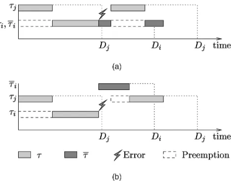
The inappropriateness of standard priority assignment approaches for error-recovery can be illustrated as follows (see Fig. 1). The figure represents a set of two hard real-time tasks, fi; jg, where the priority of j is higher than the

priority of i. Associated with i is its alternative task,i,

which should be executed in case of errors ini and must

finish byi’s deadline,Di. Consider that an error interrupts

the execution ofi, which means that the error is raised ini.

As can be seen from the scenario illustrated in Fig. 1a, it is not possible to recoveribefore its deadline because of

preemp-tion due to the execupreemp-tion ofj. Nevertheless, if there is enough

slack time available at some higher priority level whereican

be executed, it may finish beforeDi, as Fig. 1b illustrates. In

this example, the preemption of the second activation ofjis

avoided by assigning a higher priority toi.

The difficulty in deriving an appropriate schedulability analysis to cope with the example illustrated in Fig. 1b comes from the fact that the worst-case scenario is not characterized by the instant when all tasks are released at once as it is in the standard response time analysis. In Fig. 1, for instance, we can note that the response time ofjin its

second activation (Fig. 1b) is higher than its response time in Fig. 1a due to extra preemption caused by the execution of i. To carry out an appropriate response time analysis

which takes these characteristics into account, we divide the calculation of task worst-case response times into three main phases. First, we derive, for each task in the task set,

. The authors are with the Real-time Systems Research Group, Department of Computer Scienc, University of York, York YO10 5DD, UK. E-mail: {gmlima, burns}@cs.ork.ac.uk.

Manuscript received 10 Oct. 2001; revised 4 Oct. 2002; accepted 3 Dec. 2002. For information on obtaining reprints of this article, please send e-mail to: [email protected], and reference IEEECS Log Number 115168.

its worst-case response time, assuming that errors interrupt the execution of other tasks but i (i.e., due to external

errors). Then, we derive its worst-case response time, assuming that i may be faulty. In other words, this is the

time necessary, in the worst-case, to meet task deadlines despite internal errors. Finally, the values of worst-case response times due to internal and external errors are used to derive the worst-case response time of tasks. This approach has already been proposed by us [14]. Here, an improved version of this approach is described1and a more appropriate notation is used. Also, in this work, we propose an optimal priority assignment algorithm to determine the priorities of alternative tasks, a problem that has not been addressed before. By optimal we mean that the algorithm finds the best priority assignment so that the number of errors tolerated (fault resilience) by the task set is maximized and the task set is considered schedulable by the analysis. For example, from Fig. 1, we can see that the priority assignment given in Fig. 1b is better than the one given in Fig. 1a since, in Fig. 1a, the task set is not schedulable. This is due to the fact that, in Fig. 1b, the spare capacity at higher priority levels is being used to recoverifrom errors, which makes the task set

more resilient to faults.

It is important to realize that the schedulability analysis and the search for the optimal priority assignment are interdependent problems and, so, the concept of optimal is relative to the considered analysis, as we now explain. The available spare capacity, necessary to assign priorities to alternative tasks, is only known after carrying out the schedulability analysis, which gives the worst-case re-sponse times of tasks. On the other hand, an optimal priority assignment can only be given after discovering the available spare capacity. This dependency cycle suggests an iterative procedure, where priorities and task response times are calculated altogether throughout the iterations. This is the basic idea of our approach.

Carrying out this iterative procedure by brute-force, which tests all possible priority combinations, is not

practical since the number of possible priority assignments is too high. For a task set withnalternative tasks, the search space is Oðn!Þ, for instance. We solve the problem of assigning priorities to alternative tasks in a very efficient way. The algorithm to do so is iterative, as suggested. However, by establishing a partial order on the alternative task’s priorities and using some properties of the derived schedulability analysis, only a few priority configurations need to be examined. Indeed, the proposed assignment algorithm reduces the search space fromOðn!ÞtoOðn2_{Þ. We}

have proven that the proposed algorithm finds the optimal priority configuration in the sense that it maximizes the system fault resilience, as seen by the proposed analysis. To the best of our knowledge, the problem of using a nonstandard priority assignment to maximize fault resi-lience has not been addressed before.

The remainder of this paper is organized as follows: The next section presents the assumed computation model. Then, some initial concepts on the use of response time analysis for fault tolerance purposes are presented in Section 3. Also, in this section, we give the main motivation by presenting an illustrative example. Section 4 presents our approach to carrying out the schedulability analysis. In Section 5, the method for finding out the optimal priority configuration is given and its optimality is proven. The algorithm to implement such a method and a proof of its correctness are given in Section 6. Results from simulation are shown in Section 7. A brief survey on related works is presented in Section 8. Section 9 presents our final comments.

2

COMPUTATIONAL

MODEL

We assume that there is a set ÿ¼ f1;. . .; ng of n tasks,

calledprimary tasks, that must be scheduled by the system in the absence of errors. Any primary taskiinÿhas a period,

Ti, a deadlineDi (DiTi), and a worst-case computation

time, Ci. Tasks can be periodic or sporadic. For sporadic

tasks, the period means the minimum interarrival time. Each primary task i can have some alternative tasks

associated with it. Each alternative task corresponds to a given action taken to recover i from a given error. Any

alternative task has a worst-case computation time, also called worst-case recovery time. For the sake of simplicity, we denotei as the alternative task ofi whose worst-case

recovery time is the largest one. Also, we assume that all alternative tasks associated withirun at the same priority

level. Hence, hereafter we do not include the details of individual alternative task per primary in the description we present. We only need to refer to i as the worst-case

alternative task in case of errors in taski.

Primary tasks are scheduled according to some fixed priority assignment algorithm (FPðÿÞ), which attributes a distinct priority to each taskiinÿ. We considerndifferent

priority levels (1;2;. . .; n), where 1 is the lowest priority level. The alternative tasks ofi are assumed to execute at

priority levels greater than or equal to i’s priority. We

denote the priority of i and i as pi and pi, respectively.

When a primary task, sayi, and an alternative task, sayj,

are ready to execute at the same priority level, we assume thatjis scheduled first.

Fig. 1. Two illustrative scenarios: (a) bothiand its recovery run at the same priority level; (b)iruns with higher priority.

Alternative tasks represent some extra processing that is necessary to recover a task from a given erroneous state caused by a fault. Errors are detected at the task level. When an error interrupts the execution of a task, the system must schedule an appropriate alternative task, which is respon-sible for carrying out the error-processing procedure and has to finish by the deadline of its primary task. If other errors take place in the alternative tasks, we assume that it is scheduled again for reexecution. We also assume that there is no cost associated with any scheduling of primary or alternative tasks. Further, we assume that all errors are detected by the system and there is no fault propagation in the value domain (i.e., faults affect only the results produced by the executing task).

The kinds of fault with which we are dealing are those that can be treated at the task level. Consider, for example,

design faults. It may be possible to use techniques such as

exception handling or recovery blocksto perform appropriate recovery actions [3], modeled here as alternative tasks. In addition, one may consider some kind of transient faults, where either the reexecution of the faulty task or the execution of some compensation action is effective. For example, suppose that transient faults in a sensor (or network) prevent an expected signal from being correctly received (or received at all) by the control system. This kind of system fault can easily be modeled by alternative tasks, which can be released to carry out a compensation action. However, it is important to emphasize that we are not considering more severe kinds of fault that cannot be treated at the task level. For example, if a memory fault causes the value of one bit to be arbitrarily changed, the operating system may fail, compromising the whole system. Tolerating these kinds of faults requires spatial redundancy (perhaps using a distributed architecture) and is not covered in this paper. Our work fits the engineering approach that uses temporal redundancy at the processor level and spacial redundancy at the system level.

We assume in the analysis that there is a minimum time between two consecutive error occurrence, TE. By finding

out the minimum value ofTE such that the system is still

schedulable, we are expressing to what extent the system is resilient to the occurrence of errors. This may be important information about the system’s fault resilience. For exam-ple, if designers are aware of such a value, they may infer how likely the system will be subject to missed deadlines due to faults in a given environment.

It is important to emphasize that the motivation for the approach taken here is to improve fault resilience. To do this, we require a measure of this resilience. The magnitude of TE is the measure employed in this paper. We assume

that the scheduling of a system to reduce TE will improve

the resilience of the system, regardless of the actual fault model employed by the application engineer. Support for the use of this metric comes from Burns et al. [5], who proved that if error arrivals are modeled by a Poison distribution (a usual and often realistic assumption), then the probability of failure during the lifetime of the system is proportional to TE (i.e., the smaller the value of TE, the

more fault resilient the system).

3

BACKGROUND AND

MOTIVATION

Schedulability analysis based on the well-known response time analysis [1] which takes into account the effects of possible faults has already been proposed [3]. In this section, we summarize this result and illustrate its limitations.

The input parameters of this analysis are: the task attributes (Ti,Di,Ci, andC); the primary task priorities (pi),

which are given by some fixed-priority assignment algo-rithm (e.g., deadline monotonic); and the assumed value of

TE. The priorities of alternative tasks are assumed to be the

same as their primary tasks (pi¼pi).

Consider that no task suffers any error. Under this particular scenario, the worst-case response time of taskiis

the time necessary to executei and all tasks j such that

pj> pi. When faults are considered, on the other hand, we

have to include in the calculation of the worst-case response time ofithe time necessary to recover the faulty task, as we

explain below.

Initially, let us consider that only one error may take place during the execution of i. Any task that may be

executing concurrently withi (includingi itself) may be

interrupted by this error. In the worst-case scenario, the error interrupts tasks just before the end of their execution and the faulty task is the one with the longest alternative task amongiand all tasks that may preempt the execution

ofi(i.e., tasks with priority greater than or equal topi). Let

us say thatkis such a task. This means that we have to add

the time to recoverk(i.e., recovery costCk) to the response

time of i. These observations lead to (1), whereRi is the

worst-case response time ofi,hpðiÞ ¼ fj2ÿjpj> pigand

hpeðiÞ ¼ fj2ÿjpjpig. SinceRiappears on both sides of

the equation, its solution is obtained, as usual, iteratively by forming a recurrence relation with R0

i ¼Ci. This iterative

procedure finishes either whenRmþ1

i ¼Rmi (the worst-case

response time of i is found) or when Rmþi 1> Di (i is

considered unschedulable).2

Ri¼Ciþ X

j2hpðiÞ Ri

Tj

Cjþ max

k2hpeðiÞ

Ck: ð1Þ

Nevertheless, errors may interrupt the execution of k

more than once. As the worst-case period of error occurrence is TE, the maximum number of errors that

may take place during the execution ofiis given bydRi_TðT_EEÞe,

which leads to (2), originally presented in [18], [3]. AsTEis

an input to the analysis,Riis given as a function ofTE, i.e.,

RiðTEÞ. Also, note that this equation is conservative in the

sense that, in practice, some of the errors may not interrupt the task with the largest recovery cost. Indeed, this conservative assumption could only hold if error occur-rences were in phase with tasks. Assuming that errors always interrupt the execution of such a task, however, simplifies the worst-case response time computation. In this work, we use the same sort of conservative assumption.

RiðTEÞ ¼Ciþ X

j2hpðiÞ RiðTEÞ

Tj

Cjþ

RiðTEÞ

TE

max

k2hpeðiÞ Ck:

ð2Þ

Now, consider a simple but illustrative example, pre-sented in Table 1, which gives a task set with three tasks. As can be seen from the solutions of (2) presented in the table, this task set is schedulable for TE ¼11 and unschedulable

for TE ¼10 since 3 does not meet its deadline

(R3ð10Þ> D3). Nevertheless, there is some slack time available at priority levelsp1 andp2 that is not being used for carrying out the execution of3.

Our goal in this work is to develop a more generic schedulability analysis, according to which we can deal with alternative tasks running at higher priority levels. By doing so we can make use of the available slack time to carry out task recoveries. This involves two steps. First, new equations that can cope with this characteristic have to be derived (Section 4). Second, an efficient algorithm to calculate the optimal priority assignment for alternative tasks must be available (Sections 5 and 6).

4

SCHEDULABILITY

ANALYSIS

Our goal in this section is to derive schedulability analysis that takes into account alternative tasks running at higher priority levels. We assume that the priorities of alternative tasks are known beforehand. This assumption will be withdrawn in Section 5. Thus, in this section, we are only concerned with finding out whether or not a given task set is considered schedulable for a given value ofTE.

A particular choice for alternative task priorities is named apriority configuration, which is defined as follows: Definition 4.1. A priority configuration, Px, is a tuple

hhx;1;. . .; hx;ni, where0hx;i< iandhx;i¼piÿpi.

As can be noted from the definition, hx;i represents the

priority increment for taski in relation to the priority ofi.

The definition of hx;i bounds the priority of i from i’s

priority to the highest priority level. For example, consider

Px¼ h0;0;. . .;0i, a priority configuration. This means that

any alternative task executes at the same priority level as the primary task with which it is associated. For

Px¼ h0;0;. . .;0;1i, all tasks execute at their original priority

level apart fromn, which executes one priority level above

its primary task. Thus, the schedulability analysis we will present is a function ofPxandTE.

This section is structured as follows: Section 4.1 illustrates and characterizes the effects of raising priorities of alternative tasks. Section 4.2 describes the equations to calculate

worst-case task response times. In Section 4.3, the effectiveness of the analysis using the example given in Table 1 is illustrated. As we will see from this example, one can achieve significant gains by using the proposed analysis.

4.1 Raising Priorities of Alternative Tasks

In order to understand the effects of raising priorities of alternative tasks, consider the set of two tasks in Fig. 2. Taskj has higher priority than i. Suppose that an error

interrupts i just before the completion of its execution

(Fig. 2a). As can be seen,i is then selected to execute with

precedence overj. As a result, the response time of j is

increased byCiand the response time ofiis decreased by

Cj (since the second execution of j is delayed). These

effects, which are not present when alternative and primary tasks have the same priority, have to be taken into account by the response time analysis.

In addition to this, it is important to realize that the worst-case scenario cannot be represented simply by taking the task with the longest alternative task as in (2). For example, consider Fig. 2b, which represents a different execution scenario for tasksiandj. Consider thatCj< Ci

and that an error interrupts the execution ofjinstead ofi.

This situation, as can be noted from the figure, leads to a longer response time for taski when compared to Fig. 2a.

This is because taskisuffers not only the interference ofj,

but also the interference of another activation of taskj.

Summing up, the characterization of the worst-case scenario is more complex than the traditional approach (by (2)). Indeed, we have to observe the worst-case interferences due to both preemption and possible errors, which may involve the recovery of lower priority tasks. For example, from the above figure, it can be noted that the worst case for taskiis when it is released at the same time as taskjand the

error interrupts the execution ofjjust before its execution. By

contrast, the worst case for taskjis when it is released just

after taski is interrupted by an error. Let us identify tasks TABLE 1

Illustration of the Limitations of (2)

according to the extra interference they cause or suffer due to errors by defining three subsets of ÿ:

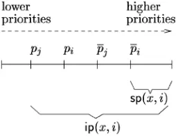
. ipðx; iÞ. These are the tasks that may interfere with

the response time of i as regards priority

config-uration Px if an error occurs. More formally,

ipðx; iÞ ¼ fj2ÿjhx;jþpjpig.

. spðx; iÞ. Tasks that belong to such a subset do not

suffer any extra interference when errors interrupt the execution ofi as regards priority configuration

Px. Their priorities are higher thanpi. More formally,

spðx; iÞ ¼ fj2ÿjpj> hx;iþpig.

. ipeðx; iÞ. This subset is defined as

ipeðx; iÞ ¼ ipðx; iÞ ifhx;i¼0

ipðx; iÞ ÿ fig ifhx;i>0:

This subset is particularly useful, as we will see in Section 4.2.2, for modeling cases where errors may interrupt taski since the maximum interference its

recovery suffers depends on whether or notpi¼pi.

Fig. 3 illustrates the meaning of subsets ipðx; iÞ and

spðx; iÞ. Note thati does not suffer any interference from

tasks in ÿÿipðx; iÞ, but suffers the interference from j

sincej2ipðx; iÞ. Thus, when calculating the response time

of i for a given priority configuration Px, we need to

consider only errors in tasks belonging toipðx; iÞ.

4.2 Task Response Time Calculation

In this section, we show how the worst-case response times of tasks are computed. Letÿbe a task set which is subject to faults so that the minimum time between error occurrences is bounded by TE>0 and assume that the priority

configuration for the alternative tasks is given by Px. The

derivation of the worst-case response time of any task

i2ÿ, denoted Riðx; TEÞ, is split into two branches:

considering that errors interrupt the execution of any task buti and considering that i may be interrupted by some

error. The justification of this approach is that the worst-case response time of any taskimay depend on whether or

not the execution of i is itself interrupted by some error

(see Fig. 2).

We call an error internal if it interrupts i (or i) or

externalif it interrupts other tasks. We defineRext

i ðx; TEÞ to

be the worst-case response time of i in cases where only

external errors are considered. In cases where some internal error takes place, the computation of the worst-case response time of i is given by Rinti ðx; TEÞ. Sections 4.2.1

and 4.2.2 describe the equations that give the values of

Rext

i ðx; TEÞandRinti ðx; TEÞ, respectively. Once the values of

Rext

i ðx; TEÞ and Rinti ðx; TEÞ are known, Riðx; TEÞ can be

easily derived (Section 4.2.3).

4.2.1 Considering Only External Errors

The computation of the worst-case response time of taski

due to external errors,Rext

i ðx; TEÞ, is straightforward. This is

because we do not need to consider the recovery ofi. In this

situation, the worst-case scenario as for task i can be

described as follows: 1) Errors take place at a rate of1=TE;

2) just before the release ofi, some alternative task with

maximum recovery time among all tasks inipðx; iÞ ÿ figis

released; and 3) all tasks inhpðiÞare released so that they cause the maximum interference in the execution of i.

Therefore, we have to take into account the time to executei

plus all tasks inhpðiÞand the time to recover the faulty task times the maximum number of errors that may occur over

Rext

i ðx; TEÞ. This scenario yields (3), which is similar to (2).

Here, we consider thatmaxk2;ðCkÞ ¼0.

Rext_i ðx; TEÞ ¼Ciþ X

j2hpðiÞ Rext

i ðx; TEÞ

Tj

Cj

þ R

ext i ðx; TEÞ

TE

max

k2ipðx;iÞÿfig

ðCkÞ: ð3Þ

It is clear that, in general, if errors arrive at eachTEtime

units, some of them may not hit the task with the largest recovery cost. However, like (2), here we make this conservative assumption for the sake of simplicity. Note that analyzing all the possibilities of error occurrences to have a less pessimistic approach may lead to a computa-tionally impractical and/or complex solution.

Not consideringiin the computation ofRexti ðx; TEÞmay

appear counterintuitive at first. Indeed, after the recovery of some faulty taskk2ipðx; iÞ ÿ fig, internal errors may take

place. However, these internal errors are only relevant for the derivation of the worst-case response time ofi when

the recovery cost of i is maximum. This is the result of

Lemma 4.1. IfCi is maximum, we need to consider these

internal errors, a problem that we address in the next section.

Lemma 4.1.Consider a fixed-priority set of primary tasksÿand their respective alternative tasks. Suppose thatÿis subject to faults so that the minimum time between error occurrences is bounded byTE >0and letPxbe a priority configuration for

the alternative tasks. If Ci<maxk2ipðx;iÞðCkÞ, R

ext i ðx; TEÞ

represents the worst-case response time of i regardless of

whether or not the execution ofiis interrupted by some error.

Proof. If just external errors take place regarding i, the

lemma holds by the explanation given earlier in this section. Hence, we have to prove that the lemma holds assuming that some internal error takes place. Thus, let us assume a hypothetical (but generic) scenario in which there is at least one internal error as fori. Without loss

of generality, definetas the time at whichiis released,

t0_{> t the time at which an internal error interrupts its}

execution, andt00_{> t}0 _{the worst-case finishing time of} i

despite other possible errors. Note that the existence oft

andt0_{is guaranteed by assumption. In this circumstance,}

there have been at most mþm0_{þ1¼ d}ðt00_ÿtÞ TE e error

occurrences, m0 of which take place during ½t; t0Þ,

one error that interrupts the execution ofiat timet0, and

m0_{¼ d}t00_ÿt

TEe ÿmÿ10error occurrences that take place

during the interval ðt0_{; t}00_{Þ (by definition of t}0 _{and t}00_).

From timetuntil timet0,isuffers the interference due to

the execution of tasks inhpðiÞ, whereas, fromt0_tot00_{, it}

suffers the interference due to the execution of tasks in

spðx; iÞ. Taking errors into account, in the worst-case:

m error occurrences interrupt the execution of a taskk

that has the longest recovery cost among all tasks in

ipðx; iÞ ÿ fig and m0 error occurrences interrupt the

execution a task l that has the longest recovery cost

among all tasks inspðx; iÞ [ fig.

Now, let us compareRext

i ðx; TEÞwitht00ÿt, where we

have to prove that Rext

i ðx; TEÞ t00ÿt. It is clear that

Rext

i ðx; TEÞ cannot be less than t0ÿt since, by

assump-tion, i was executing at t0 and, during this interval of

time, (3) takes into account the worst-case interference. In other words, (3) takes into account at least: mþ1 error occurrences during ½t; t0_{Š and the same amount of}

interference caused by alternative and primary tasks that may preempt i during ½t; t0Š. From t0 onward,

however, (3) takes into account external errors in taskl.

Sincespðx; iÞ ipðx; iÞ,Ci< Ck, andClCk, (3) cannot

converge to a number smaller thant00_{ÿt, as required.tu}

Although we do not need to carry out the computation of

Rint

i ðx; TEÞwhenCi<maxk2ipðx;iÞðCkÞ, we will do so for the

sake of illustration. This means that the equations we derive in the next section will take into account scenarios ruled out by Lemma 4.1.

4.2.2 Considering Internal Errors

In this section, we assume that there is at least one internal error during the execution of i. The general strategy for

deriving Rint

i ðx; TEÞ is illustrated in Fig. 4. As can be seen

from the figure, an internal error takes place at timetwhich releasesi. The interference thati andi suffer due to the

execution of other tasks may be different if pi< pi, as is

illustrated in the figure. The objective of the analysis is to derive the worst-case response times ofi before and after

the error. We call these times Rint0

i ðx; TEÞ and Rint

1

i ðx; TEÞ,

respectively.

Deriving the values ofRint0

i ðx; TEÞandRint

1

i ðx; TEÞis not

simple since: 1) This may involve two levels of priorities,

before and after the first internal error; 2) the procedure to carry out response time analysis is iterative; and 3) the information aboutwhenthe first internal error takes place is not available beforehand. In other words, in general,

Rint0

i ðx; TEÞand Rint

1

i ðx; TEÞ cannot both be derivedat once

using response time analysis.

In order to circumvent difficulties 1) and 2), we compute the values of Rint0

i ðx; TEÞ and Rint

1

i ðx; TEÞ separately. This

strategy makes it easier to use response time analysis for taking into account the different interference in both priority levels, before and after the error. The final result of Rint

i ðx; TEÞ can then be given by the sum ofRint

0

i ðx; TEÞ

and Rint1

i ðx; TEÞ, as we will see. Due to difficulty 3), we

carry out the following approach: First, we suppose that the execution ofiis interrupted by an error at some timet(as

illustrated in Fig. 4). Then, we can easily deriveRint1

i ðx; TEÞ.

Note that this derivation does not need any information about what happened beforet. Then, using the computed value of Rint1

i ðx; TEÞ, we derive Rint

0

i ðx; TEÞ. We detail this

approach below. Computing Rint1

i ðx; TEÞ. Here, we assume that an

internal error took place. What we have to do is to show how long the recovery ofi will last subject to both other

possible errors and the interference due to tasks inspðx; iÞ. In the worst-case, there may be dRint

1 i ðx;TEÞ

TE e errors over the

periodRint1

i ðx; TEÞ. The first error accounts forCi, while the

others may cause the release of the recovery of any task in

spðx; iÞ [ fig. The worst case is when all other errors

interrupt a task in spðx; iÞ [ fig that has the longest

recovery time.3Therefore,Rint1

i ðx; TEÞis given by (4).

Rint1

i ðx; TEÞ ¼Ciþ X

j2spðiÞ Rint1

i ðx; TEÞ

Tj

& ’

Cj

þ R

int1

i ðx; TEÞ

TE

& ’

ÿ1

!

max

k2spðx;iÞ[fig

ðCkÞ: ð4Þ

ComputingRint0

i ðx; TEÞ. The computation ofRint

0

i ðx; TEÞ

is slightly more complex. Let us analyze it considering two cases depending on the values ofpiandpi.

When pi< pi. This means that i executes at a higher

priority level. Note that, in this case, knowingRint0

i ðx; TEÞ

is equivalent to knowing the relative earliest possible release time ofiso that it suffered the first internal error

at timet, as illustrated in Fig. 4. During Rint0

i ðx; TEÞ,i

may suffer the preemption of tasks inhpðiÞand possibly the recoveries of tasks in ipðx; iÞ ÿ fig due to other

errors. It is important to note that we have to removei

from the set of tasks that may suffer errors in this phase because, by assumption, the first error occurs at timet. Indeed, if there was an earlier internal error, then i

would be released earlier and, so, it would finish earlier. It is clear that this situation does not represent the worst-case scenario.

3. As said before, here we are assuming a generic situation. However, in practice, one can consider that all errors fromtonward are internal due to Lemma 4.1.

When pi ¼pi. Unlike the former case, the maximum

interference duringRint0

i ðx; TEÞ can take place when all

errors are internal since bothi and its alternative task

run at the same priority level. This situation happens, for example, when Ci¼maxk2ipðx;iÞðCkÞ (recall (2)). As a

result, instead of considering errors inipðx; iÞ ÿ fig, one

should consider errors in the wholeipðx; iÞ. In summary, as for possible errors during Rint0

i ðx; TEÞ,

when pi< pi, one has to consider errors in ipðx; iÞ ÿ fig.

Otherwise, errors in ipðx; iÞ should be taken into account. This is the main difference between the cases analyzed above. In order to join both cases together in a single equation, we say that errors during the intervalRint0

i ðx; TEÞ

may take place in any task inipeðx; iÞ(see Section 4.1). Now, we are able to derive the equation that gives

Rint0

i ðx; TEÞ. It has to take into account: the worst-case

execution time of i (Ci), the interference due to tasks in

hpðiÞ, and possible recoveries of tasks inipeðx; iÞ. Note that some releases of tasks inspðx; iÞand some error occurrences may have already been taken into account when computing

Rint1

i ðx; TEÞ. This means that we have to take care not to

compute the same task in spðx; iÞ and the same error occurrence twice. In other words, we have to subtract, for each task in spðx; iÞ and each error occurrence, the interference already computed inRint1

ð iÞðx; TEÞ.

From the description above, (5) gives the value of

Rint0

i ðx; TEÞ. Note that, instead of computing the worst-case

interference due to tasks inhpðiÞ, we split this computation as for two complementary subsets, hpðiÞ ÿspðx; iÞ and

spðx; iÞ. This is to avoid the computation of tasks in

spðx; iÞ more than once, as commented before. We do so by subtracting dRint

1 i ðx;TEÞ

Tl eCl for each task l2spðx; iÞ.

Similarly, possible double counting of errors is removed by subtractingdRint

1 i ðx;TEÞ

TE efrom the total number of errors.

Rint_i 0ðx; TEÞ ¼Ciþ X

j2hpðiÞÿspðx;iÞ Rint0

i ðx; TEÞ

Tj

& ’

Cjþ

X

l2spðx;iÞ Rint

i ðx; TEÞ

Tl

ÿ R

int1

i ðx; TEÞ

Tl

& ’!

Clþ

Rint i ðx; TEÞ

TE

ÿ R

int1

i ðx; TEÞ

TE

& ’!

max

k2ipeðx;iÞ

ðCkÞ:

ð5Þ

The value of Rint

i ðx; TEÞ can then be simply derived by

taking the sum ofRint0

i ðx; TEÞandRint

1

i ðx; TEÞ:

Rint_i ðx; TEÞ ¼Rint

0

i ðx; TEÞ þRint

1

i ðx; TEÞ: ð6Þ

The computation ofRint

i ðx; TEÞis carried out by iteration as

usual. Initially, the calculation of Rint1

i ðx; TEÞ is done and

then its value is used in (5). Notice that the procedure for calculating Rint0

i ðx; TEÞ does not affect the value of

Rint1

i ðx; TEÞ.

4.2.3 Worst-Case Response Time

In this section, we show how to deriveRiðx; TEÞ, the

worst-case response time ofi, fromRexti ðx; TEÞandRinti ðx; TEÞ. In

order to give an intuition behind this derivation, let us

analyze two cases below. Considerka task inipðx; iÞsuch

thatCk¼maxl2ipðx;iÞðClÞ.

If k2ipðx; iÞ ÿ fig. In this case, Rinti ðx; TEÞ is maximum

when all errors hit taskkor some other taskl(or their

alternative tasks) that has recovery cost equal toCk. This,

in turn, can only be true ifkorlbelong tospðx; iÞ. Without

loss of generality, assume that k2spðx; iÞ. Hence, the

computation ofRint

i ðx; TEÞ takes into account mÿ10

error occurrences regardingkand one fori, wheremis

the maximum number of errors that may occur during

Rint

i ðx; TEÞ. Clearly, this represents the worst-case scenario

when some internal error takes place. However, as the computation of Rext

i ðx; TEÞ takes into account all error

occurrences fork,Rexti ðx; TEÞassumes a value at least as

big asRint

i ðx; TEÞ. Indeed, ifCi< Ck, by Lemma 4.1, we

know thatRext

i ðx; TEÞ Rinti ðx; TEÞ. Moreover, ifCi¼Ck,

it is not difficult to see thatRext

i ðx; TEÞ Rinti ðx; TEÞsince

spðx; iÞ hpðiÞ. Therefore,Riðx; TEÞ ¼Rexti ðx; TEÞ.

Ifk¼i. In this case, the computation of Rinti ðx; TEÞ takes

into account some errors in another task l2ipðx; iÞ ÿ figand some in i. SinceRinti ðx; TEÞ depends on pi,pi,

Ci, and Cl, the relation between Rexti ðx; TEÞ and

Rint

i ðx; TEÞ is unknown before the computation of their

values. In other words, in this case,Riðx; TEÞis given by

the maximum ofRext

i ðx; TEÞandRinti ðx; TEÞ.

Therefore, the generic expression that gives the value of

Riðx; TEÞis straightforwardly given by

Riðx; TEÞ ¼maxðRexti ðx; TEÞ; Rinti ðx; TEÞÞ: ð7Þ

To conclude this section, we call the attention of the reader to the fact that the described analysis represents a generalization of the analysis by (2). This is proven by the lemma below.

Lemma 4.2. Consider a set of fixed-priority scheduled set of primary tasksÿand their alternative tasks. For any value of TE>0, the worst-case response time given by (2) equals the

m axi mu m o f Rext

i ðx; TEÞ a n d Rinti ðx; TEÞ w h e n e v e r

Px¼ h0;0;. . .;0i.

Proof. The proof of this lemma is straightforward and follows the observation that, when Px¼ h0;0;. . .;0i,

hpðiÞ ¼spðx; iÞ and ipeðx; iÞ ¼hpeðiÞ ¼ipðx; iÞ. After some simple algebra, (3) and (6), respectively, can be rewritten as follows:

Rext_i ðx; TEÞ ¼Ciþ X

j2hpðiÞ Rext

i ðx; TEÞ

Tj

Cj

þ R

ext i ðx; TEÞ

TE

max

k2hpðiÞ

ðCkÞ

and

Rint

i ðx; TEÞ ¼Ciþ X

j2hpðiÞ Rint

i ðx; TEÞ

Tj

Cj

þ R

int i ðx; TEÞ

TE

ÿ1

max

k2hpeðiÞ

ðCkÞ þCi:

Ci¼ max k2hpeðiÞ

ðCkÞ;

Rint

i ðx; TEÞ Rexti ðx; TEÞ. Otherwise,

Rint

i ðx; TEÞ Rexti ðx; TEÞ:

The maximum of these two equations can then be rewritten as a single equation, which yields (2). tu

4.3 An Illustrative Example

As we have seen, whenTEis set to 10 time units, the task set

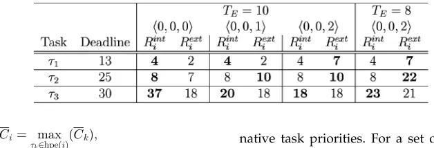
presented in Table 1 is unschedulable for priority configura-tionh0;0;0i. Table 2 shows that, for priority configurations

h0;0;1iandh0;0;2i, the task set is schedulable according to the analysis described earlier. This is because the slack time available at higher priority levels is being used to execute3.

The two values given in each cell of Table 2 are the solutions of (6) and (3), respectively. The maximum value (i.e., the worst-case response time) is in bold.

The advantages of considering alternative tasks execut-ing at higher priority levels are not only noted from the significant reductions of task response times, but also from the increase in the fault resilience of the task set. In this example, the value of TE drops from 11 (priority

config-uration h0;0;0i) to 8 (priority configuration h0;0;2i), as illustrated in the table. This represents a gain of 27.3 percent, which may be very significant when dealing with critical applications.

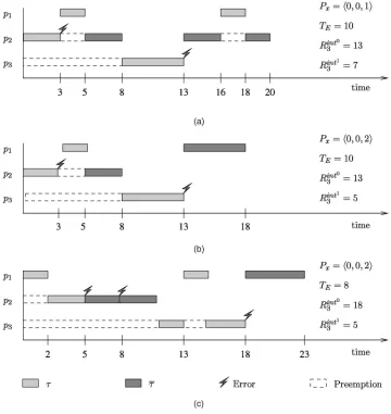
Fig. 5 illustrates some examples of scheduling that lead to the worst-case response times of 3 when an internal error takes place. Scenarios (a), (b), and (c) correspond to the three last columns of Table 2, respectively. Let us focus on scenario (c) in the figure and compare with the values given by the analysis. By (4) and (5), Rint1

3 ðx;8Þ ¼5 and Rint0

3 ðx;8Þ ¼18, respectively. This is because the analysis

takes into account two errors as for2and one internal error in3. It is clear that2(or its recovery) cannot be interrupted by two errors since its period is 25 and TE¼8. This

approximationis the result of our conservative assumption, which says that any error always interrupts the task with the longest recovery time among all tasks that may interfere in the execution of 3 (in this case). The approximation is represented in the figure as if there were two consecutive executions of 2. Similar consequences of this assumption can also be seen in both (2) and (3), as noted earlier.

Up to now we have not been concerned with determin-ing the best priority configuration so that the fault resilience of the task set is minimized. The difficulty in finding such anoptimalpriority configuration is twofold. First, there are a huge number of possible different arrangements of

alter-native task priorities. For a set of n tasks (one alternative task per primary task), this number isn!since there aren

possible priority values for the lowest priority task, nÿ1

for the second lowest priority task, and so on. Second, the search for the optimal priority configuration depends on the slack time available in higher priority levels, which, in turn, depends on the worst-case response times of tasks. The next section addresses this problem and presents an efficient solution to it.

5

THE

PRIORITY

CONFIGURATION

SEARCH

METHOD

A description of the method to find out the optimal priority configuration regarding the analysis described earlier is given in this section. The main idea behind the method can be summarized as follows: Based on some properties of the analysis, an iterative procedure transforms a given priority configuration, say Px, into another, say Py, where Py is a

potential optimization of Px. We say that Py is an

optimization ofPxif smaller values of TE may be used on

Py without causing any task to miss its deadline. The

procedure for improving a priority configuration is based on raising the priority of the alternative tasks that are causing the unschedulability of the task set. These tasks are calleddominant tasks(Section 5.1). This iterative procedure stops when it is no longer possible to carry out any improvement. In order to search for optimized priority configurations from the initial configuration, apartial order

of priority configurations is established (Section 5.2). The search is carried out in ascending order of priority configurations and it chooses those that could potentially reduce the value of TE. The great advantage of this

approach is that we do not need to consider all possible priority configurations, which would be too expensive. Only a small number of possibilities are checked.

5.1 Dominant Tasks

A given priority configuration, say Px, has a minimum

allowed value of TE, denoted by the function TeðxÞ. If any

value less thanTeðxÞis attributed toTE, some task may be

unschedulable. In particular, ifTE¼TeðxÞ ÿ1, then there is

at least a task i in ÿ such that Riðx; TeðxÞ ÿ1Þ> Di. The

tasks that cause the unschedulability of ÿ under this circumstance are called dominant tasks. We distinguish two kinds of dominant task: 1-dominant and 2-dominant. A taskiis 1-dominant regarding the priority configurationPx

if Rint

i ðx; TeðxÞ ÿ1Þ> Di. Two-dominant tasks are those

tasks that may cause other tasks to miss their deadlines when TE¼TeðxÞ ÿ1 because of the execution of their

alternative tasks. Below, we define more formally the

TABLE 2

concept of dominant tasks and give the definition of their respective task sets.

Definition 5.1. A task i is a dominant task in relation to a

priority configurationPxifiis 1-dominant, i.e., it belongs to D1_{ðxÞ, or 2-dominant, i.e., it belongs toD}2_{ðxÞ, where}

D1_ð

xÞ ¼ i2ÿjRinti ðx; TeðxÞ ÿ1Þ> Di

and

D2_{ðxÞ ¼}

i2ÿj 9j2ÿ :i 2ipðx; jÞ ^

Rext_j ðx; TeðxÞ ÿ1Þ> Dj ^Ci¼ max k2ipðx;jÞ

ðCkÞ

:

Therefore, optimizing a priority configuration means reducing the worst-case response times due to internal errors of all 1-dominant tasks. Worst-case response times due to internal errors can only be reduced by increasing alternative task priorities. Table 2 illustrates this, where the

Rint

3 ðx;10Þis decreased whenp3is increased. This is because

the size ofspðx;3Þis reduced and, so, the interference due to preemption over the execution of3 is reduced as well. As for 2-dominant tasks, there is no space for optimization by raising the priorities of their alternative tasks. This is

because doing so does not decrease the interference 2-dominant tasks cause in other tasks.

Table 3 shows the worst-case response times due to internal and external errors for three different configura-tions with regard to the task set of Table 1. The symbol “” means that the task is unschedulable. The minimum allowed value ofTE in h0;0;0i is 11 time units, where 3

is 1-dominant. Increasing the priority of 3 by 1 leads to

h0;0;1i, which makesTeðh0;0;1iÞ ¼8. Note that, in priority

configuration h0;0;1i, 3 is 2-dominant since it makes 2

unschedulable for TE¼7. Since Rext2 ðx;7Þ cannot decrease

by raising p3 further, from h0;0;1i no optimization is possible.

As can be noted from Table 3, the reduction of

Rint

i ðx; TEÞ, where i is some 1-dominant task, plays an

important role in optimizing priority configurations. How-ever, sometimes it is not possible to decreaseRint

i ðx; TEÞby

raising the priorities of alternative tasks. For example, if2

ran at the highest priority level in the priority configuration

Px¼ h0;1;0i,Rint2 ðx; TEÞ would still be eight time units. A

similar situation occurs with Rint

3 ðx; TEÞ regarding priority

configurations h0;0;1i and h0;0;2i. Let us formalize this property by means a condition, which is a direct conse-quence of (4) and (5).

Fig. 5. Illustration ofRint

Consider a priority configuration, sayPx.Rinti ðx; TEÞcan

be reduced by increasing pi if the following improvement

condition holds:

Condðx; i; jÞ 9j2spðx; iÞ:

Rint i ðx; TEÞ

Tj

> R

int0

i ðx; TEÞ

Tj

& ’

: ð8Þ

This condition means that all preemption on the execution oficaused by the releases ofjcan be eliminated if we set

pi pj. We use the predicate above to avoid checking all

configuration priorities in the optimization procedure. Only those that may reduce the values of 1-dominant task worst-case response times due to internal errors (where the predicate is true) need to be checked. It is important to note that this condition is necessary (but not sufficient) to optimize priority configurations. The next section presents the method used for such an optimization.

5.2 Search Graph and Search Path

Consider tasksiandjinÿ, a given priority configuration

Px andTE>0. Raising the priority ofi, as we have seen,

may decrease the value ofRint

i ðx; TEÞ, but cannot decrease

the value ofRext

i ðx; TEÞ. Also, ifi2ipðx; jÞ ÿhpðjÞ, raising

the priority of i may increase the value of Rextj ðx; TEÞ.

Hence, in general, we can say that the maximum worst-case response times considering internal errors and the mini-mum worst-case response times due to external errors is when all alternative tasks run at the same priority level as their respective primary tasks, i.e., when the priority configuration equals h0;0;. . .;0i. Conversely, when all alternative tasks run with the highest possible priority, i.e., priority configuration h0;1;. . .; nÿ1i, we have the minimum worst-case response times due to internal errors, but the maximum values of worst-case response times due to external errors. As the schedulability of any task i is

given by the maximum of Rint

i ðx; TEÞ and Rexti ðx; TEÞ, we

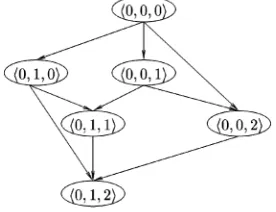
have to search the optimal priority configuration in the interval h0;0;. . .;0i and h0;1;. . .; nÿ1i. Based on this observation, let us order the set of all possible priority configurations by means of a direct acyclic graph, thesearch graph, where the priorities configurations h0;0;. . .;0i and

h0;1;. . .; nÿ1i are in the first and last position of such an order, respectively.

Definition 5.2. A search graph SG¼ fV ; Eg is a direct acyclic graph. Its vertex set is a set of n! vertices, V ¼ fv0; v1;. . .; vn!ÿ1g, where each vx is labeled with the

priority configurationPx. Its edge set is defined as

E¼ fðvx; vyÞ 2V Vj 91j;8i6¼j:

hx;i¼hy;i^hx;j< hy;jg:

Fig. 6 illustrates the search graph for a set of three tasks. It can be seen from the graph that the vertex labeled

h0;0;. . .;0i does not have any incoming edges and the vertex labeled h0;1;. . .; nÿ1i does not have any outcome edges. We name these vertices the source (v0) and the sink

vertices (vn!ÿ1), respectively. The order shown in the graph

is expressed by the relation_e>_{, which is defined below.}

Definition 5.3.Letvx andvybe two vertices of a search graph

SG. We say thatvyis reached fromvx, denotedvx_e>v_y, if and only if x¼y or there is a path in SG fromvx to vy. More

formally, xx_e>vy, ðx¼yÞ _ ðvx;. . .; vyÞ 2SG, where ðvx;. . .; vyÞis a path inSG.

Consider the search graph presented in Fig. 6. Letvxbe a

given vertex of the search graph and Px its associated

priority configuration. The problem we will now address can be stated as follows:Is there any vertexvy, wherevx_e>vy,

such that its associated priority configuration,Py, makes the task

set schedulable with TE < TeðxÞ? Suppose, for instance, that

Px¼ h0;0;1i has two 1-dominant tasks, 2 and 3. In this

scenario, only the sink vertex may optimize Px provided

that 1) the task set is schedulable in such a priority configuration withTE < TeðxÞand 2) it is possible to reduce

Rint

2 ðx; TEÞ and Rint3 ðx; TEÞ. This is because it is necessary

(but not sufficient!) that both 2 and 3 run with higher priorities than their priorities inPx. Consider now that only

3is dominant. Thus, we can guarantee that neitherh0;1;0i

norh0;1;1i can optimize Px since the priority of3 is not

increased in those priority configurations. If 3 is 1-dominant, h0;0;2i may be an optimization of Px.

How-ever, if3is 2-dominant, no improvement is possible (recall that3 is causingRext

1 ðx; TEÞ> D1orRext2 ðx; TEÞ> D2). Let

us now takePx¼ h0;0;0iand let us look at the possibilities

to optimize Px. If the only 1-dominant task is 3, either h0;0;1i orh0;0;2imay optimize Px. Which one is the best

choice? To answer this question, we have to look at the improvement condition, (8). Ifh0;0;1idoes not satisfy this condition, we try h0;0;2i. Otherwise, h0;0;1i is a better choice since we avoid increasing the priority of3too much.

If other improvements are possible from h0;0;1i, similar analysis will lead toh0;0;2ior even further toh0;1;2i.

As can be seen, if we start searching for the optimal configuration from the source vertex, we only need to carry optimization with respect to increasing in priorities. The idea is to keep decreasing the worst-case response times

TABLE 3

Worst-Case Response Times Due to Internal and External

Errors whenTE¼TeðxÞ ÿ1

due to internal errors of 1-dominant tasks through a path from the source vertex. The last vertex of this path is one that can no longer be improved (either because it is the sink vertex or because the improvement condition is not true). We call this path thesearch path.

Definition 5.4.A search pathSP ¼ ðv0; v1;. . .; vwÞis any path

in SG beginning from the source vertex such that, for all edges

ðvx; vyÞ 2SP, there is a 1-dominant taskiwith regard toPx

such that

Rint_i ðx; TeðxÞ ÿ1Þ> Rinti ðy; TeðxÞ ÿ1Þ ð9Þ

and

hy;i¼ min

ðvx;vzÞ2SG hz;i

ÿ

: ð10Þ

If an edge belongs to a search path, it leads to a priority configuration which reduces the value of Rint

i ðx; TeðxÞ ÿ1Þ

for a given 1-dominant taski (by (9)) and such a priority

configuration has the minimum possible value ofpi(by (10)).

Consider the task set given in Table 1. Its search path,

ðv0; v1Þ, is shown in Fig. 7. In h0;0;0i, we know that 3 is 1-dominant. Observing the definition of the search path, we move to h0;0;1i. Note that h0;0;1i is the last priority configuration in the path since there is no other 1-dominant task. Also, observe that, even if3 were 1-dominant in this priority configuration, its worst-case response time could not be decreased (recall Table 3 and the improvement condition).

Summing up, in order to find out an optimal priority configuration one has to follow a search path. This is formalized by the theorem below.

Theorem 5.1. Consider ÿ a fixed-priority scheduled set of primary tasks and their respective alternative tasks. Suppose thatÿis subject to faults so that the minimum time between error occurrences is bounded by TE>0. Let SP ¼ ðv0; v1;. . .; vwÞbe a search path in a search graph SGas for

tasks in ÿ. The priority configurationPx such that TeðxÞ ¼

min8vz2SPðTeðzÞÞ is the minimal value of TE such that Riðx; TeðxÞÞ< Di for any taski2ÿ.

Proof. Assume by contradiction that there is a priority configuration Py6¼Px such that TeðyÞ< TeðxÞ and

Riðy; TeðyÞÞ< Di for any task i 2ÿ. If vy2SP, then

the proof is trivial. Consider that vy62SP. This means

that: 1)8i2 D1ðxÞ:hy;i> hx;iand 2)8j2 D2ðxÞ:hy;j<

hx;j since these conditions are necessary for decreasing

t h e v a l u e o f TE ¼TeðxÞ. C o n s i d e r t h e p a t h

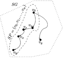
P ¼ ðvx;. . .; vwÞ SP. See Fig. 8, where the dotted line

represents the search graph and the dashed line represents the search path. By the definition of the search path, all vertices inP have increased the priority of the alternative task of some dominant task in D1_ðxÞ

and, from Pw, it is no longer possible to reduce any

dominant task worst-case response time due to internal errors by increasing the priorities of alternative tasks. SincePy exists (by assumption), TeðxÞ (by definition) is

minimum in SP and 1) holds, we conclude that

D1_{ðxÞ ¼ ;}

. Now, consider D2_{ðxÞ 6¼ ;}

. Without loss of generality, consider some j2 D2ðxÞ. Thus, there is an

edgeðvu; vsÞinSP such thathy;j¼hu;j, making the value

hs;j too high. By (10),hs;j is the minimum necessary to

decrease Rint

j ðu; TeðuÞ ÿ1Þ (note that j2 D1ðuÞ). Any

priority configuration with the same value ofhu;jcannot

be schedulable usingTE < TeðuÞ sincej is a dominant

task inPu. Therefore, sinceTeðxÞis minimum inSP and ðvu; vsÞ 2SP, TeðxÞ TeðuÞ TeðyÞ, which provides the

contradiction. tu

6

THE

ALGORITHM

Theorem 5.1 proves the correctness of the method for finding out the optimal configuration based on the concepts of search graph and search path. This section presents an algorithm to implement such a method. As we will see, its execution is equivalent to traversing a search graph through a search path up to a point at which some task becomes 2-dominant. However, it is not necessary to use the implementation of the search graph itself. This approach would be too expensive since the search graph has

n! vertices. The intuition behind the algorithm is to make

TE¼TeðxÞ ÿ1 for a given priority configuration Px and

then to look for a priority configuration Py(wherevx_e>vy)

which makes the task set schedulable with such a value of

TE. If such aPyexists, the algorithm finds it. Otherwise, the

algorithm stops. This procedure is iterative and starts with

Px¼ h0;0;. . .;0i.

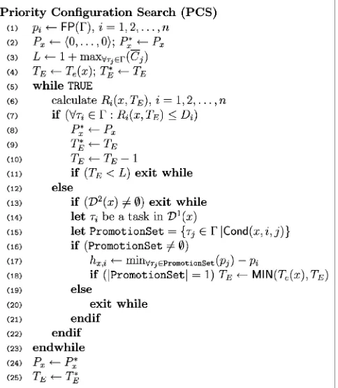
The algorithm is straightforward (see Fig. 9). First of all, some initialization is done in lines 1-2. Then, the lower boundL onTE and the minimum value for TE regarding

the initial configuration are calculated (lines 3, 4, and 5, respectively). The value ofLis set to1þmax8j2ÿðCjÞ. This

Fig. 7. The search path for the task set given by Table 1.

is because, if TE assumes lower values, in the worst-case,

the same alternative task is always interrupted by an error. This means that the task with the longest recovery cost never completes, which implies that the task set is unschedulable. The initial priority configuration Px and

the found value of TeðxÞ is saved in variables Px and TE,

respectively. This is necessary in cases where the task set is unschedulable in h0;0;. . .;0i. These values will change throughout the execution of the search algorithm if some optimal priority configuration is found. Otherwise, P0¼ h0;0;. . .;0i andTeð0Þare returned as default values. After

the initialization, the optimization procedure is carried out (lines 5-23) until no optimization is possible (lines 13 or 20) orTE< L(line 11).

The iterative search has two blocks, the save-block (lines 8-11) and the promotion-block (lines 13-21). When-ever the task set is schedulable, the save-block is executed in order to save both the last improved priority configuration and the minimum value found for TE regarding such a

priority configuration. Each execution of the save-block is followed by the execution of the promotion-block. This is because line 10 guarantees that the task set will not be schedulable in the next iteration.

Whenever the task set is considered unscheduled and there are no 2-dominant tasks, the promotion-block is executed. If there is some 2-dominant task, the algorithm stops. In line 14, some 1-dominant task is selected for promotion. Note that any 1-dominant task can be selected. Then, the improvement condition is checked since this is necessary for decreasing the worst-case response time due to internal errors of the selected dominant task. If there is no task that satisfies the improvement condition (i.e., PromotionSet _{is empty), the search stops and the last}

saved configuration is optimal. Otherwise, the promotion of the alternative task of the selected dominant task is carried out (line 17). Note that its alternative task priority is set to the lowest priority level, which allows a smaller value of the worst-case response times due to internal errors. Then, in line 18, a new value of TE is calculated. This is necessary

because, ifPromotionSet_{is a unitary set, the promotion} carried out in the earlier line may reduce the value ofTeðxÞ.

The value of TeðxÞmay increase throughout the

optimiza-tion process if the selected 1-dominant task becomes 2-dominant. In this case, the algorithm stops in the next iteration in line 13.

We have assumed up to now that the valueTeðxÞfor any

priority configurationPxis available. Indeed, this function

can be implemented straightforwardly as a binary search. The initial search interval can be set to½L;max8iðDiފ. As

we mentioned earlier,TE cannot assume values less thanL

without compromising the schedulability of the task set. If

TEmax8iðDiÞ, only one error occurrence within the

longest response time of the task set may take place. If the task set is unschedulable with this maximum value, it will be unschedulable with errors occurring at any rate.

It is interesting to note that it is possible to improve the implementation of the algorithm by making two slight changes. The first is with respect to the implementation of the functionTeðxÞ. As can be seen, we only set a new value

to TE in line 18 if the priority configuration is optimized.

Thus, we can reduce the search interval for the binary search to½L; TEŠ, whereTE is its current value. The second

modification is related to the choice of the dominant task in line 14. Although any 1-dominant task can be selected, it is preferable to select one, sayi, with the highest alternative

task priority. This is because the possibility of reducing

Rint

i ðx; TEÞis lower, which may lead to a smaller number of

iterations when it is not possible to improve priority configurations.

6.1 Proof of Correctness and Complexity

In order to prove the correctness of the PCS algorithm, we have to show that 1) an optimal priority configuration is found (Theorem 6.1) and 2) the algorithm stops (Theorem 6.2). Before showing this, the equivalence between search path and the execution of the algorithm is shown (Lemma 6.1).

Lemma 6.1.LetS¼ ðP0; P1;. . .; PwÞbe the sequence of priority

configurations generated by the algorithm PCS.Sis a prefix of or is equal to the label sequence of a search path SP ¼ ðv0; v1;. . .; vwÞ.

Proof. First, suppose that, during the execution of the algorithm, no task becomes 2-dominant. In this case, we prove by induction thatS is the exact sequence of the vertices inSP. The induction is on the number of times that the algorithm executes the promotion-block. The base case is the first execution of the promotion-block. Note that the execution of the save-block does not change the priority configuration. It is clear thatv0, labeledP0¼ h0;0;. . .;0i, belongs to the search path by definition. SinceD2_{ð0Þ ¼ ;}

, during the first execution of the promotion-block either the algorithm stops (PromotionSet_{¼ ;) and, so,jSj ¼ jSPj ¼} 1or a promotion is carried out. Let P1 be the second

priority configuration in S. By definition of the search path, P1 is the label of v1 since (10) corresponds to the execution of line 17 and (9) holds because

PromotionSet_{6¼ ;. Hence, the base case holds. Now,}

suppose that a given Px2S is the label of vx so that ðPx; PwÞ 2S and ðvx; v0wÞ 2SP. By the algorithm, this

means that line 17 was executed and the promotion of a dominant task was carried out. By a similar argument made for the base case, this promotion is equivalent to traversing an edge inSP and, so,Pwis the label ofv0w, i.e.,

v0_w¼vw. Therefore, if no 2-dominant task is found during

the execution of the algorithm, the sequence S is the exact sequence of a givenSP. Now, consider that some 2-dominant task is found in some priority configuration

Px2S. As a result, by line 13, the algorithm stops inPx.

Observe that, in this case, Px is the last priority

configuration in S and the first one such that

D2_{ðxÞ 6¼ ;. Hence, by the induction above, it is clear that}

there existsvx2SP andPxis the label ofvx. As a result,

the sequenceðP0; P1;. . .; PxÞis the label of the vertices of

the subsequence ðv0; v1;. . .; vxÞ 2SP. Therefore, S is a

prefix of the label sequence ofSP, as required. tu

Theorem 6.1.The algorithm PCS finds an optimal configuration priority regarding the proposed analysis.

Proof.Based on the results of Lemma 6.1 and Theorem 5.1, we only need to show that the last saved configuration corresponds to the optimal one. By the algorithm,P0¼ h0;0;. . .;0i is the first saved priority configuration. Assume first that there is no other execution of the save-block. This is because the algorithm stops in line 11, 13, or 20, which means that no optimization was possible from P0. In other words, for any other priority config-uration reached by the algorithm, sayPz, the task set is

unschedulable with TE¼Teð0Þ ÿ1. As a result, P0 is

optimal. Now, assume that there are at least two (consecutively) saved priority configurations, Pyand Px

say. By the construction of the algorithm, the values attributed to TE do not increase throughout the

itera-tions. Thus,TeðxÞ TeðyÞ. This implies that the last saved

priority configuration has the minimum (optimal) value

ofTE, as required. tu

Theorem 6.2.The algorithm PCS stops with at most nðnÿ1Þ

iterations.

Proof.By construction of the algorithm, it stops either when

PromotionSet_{¼ ; or when L > TE or when the}

algo-rithm reaches some configuration with a 2-dominant task. Let us assume that there is some task set that does not have any 2-dominant task for all possible priority configurations. In this case, the algorithm never stops due to 2-dominant tasks. AsLTE is a precondition of

the algorithm which is guaranteed to be true throughout the iterations (line 11), we have to prove that the condition PromotionSet_{¼ ; is eventually true at most}

at the iteration number nðnÿ1Þ. Our proof will be by looking at the longest possible search path in the search graph (using the result of Lemma 6.1). By the definition of the search graph, the longest path isðv0; v1;. . .; vn!ÿ1Þ.

If this path is the longest one, it is characterized by increasing one task priority level per edge. Thus, for the

lowest priority task, we have to traversenedges, for the second lowest priority task,nÿ1edges, and so on. The maximum number of traversed edges is

Xnÿ1

i¼1

i¼nðnÿ1Þ

2 :

The worst case is when there is only one 1-dominant task in each vertex of the search path and each promotion of its priority makes the task set schedulable (i.e., each execution of the promotion-block is followed by one execution of the save-block). As a result, two iterations per priority promotion are necessary, one to promote the priority of a dominant task and the other to save the priority configuration. As each promotion is equivalent to traversing an edge of the search graph, the maximum number of iterations is twice the maximum number of traversed edges. Also, for the priority configuration

h0;1;. . .; nÿ1i, PromotionSet_{¼ ; since all alternative}

tasks are executing in the highest priority level. There-fore, there are at mostnðnÿ1Þiterations. tu

The time complexity of the search is determined by the worst-case number of iterations, i.e., Oðn2_{Þ. This can be}

considered a significant result since we reduced the search space from n! to n2_{. The whole algorithm has time}

complexity nearly Oðn4_{Þ since, in the worst case, we have}

to calculate the response time (line 23)n2 _{times and carry}

out the sensitivity analysis (functionTeðxÞ—line 18)

when-ever the promotion block is executed.

7

ASSESSMENT OF

EFFECTIVENESS

This section characterizes the applicability of the described approach by simulation, where 18,000 task sets (10 tasks per task set) were generated. The values of worst-case compu-tation time and recovery costs of each task set were generated according to an exponential distribution with mean U=10, where U is the processor utilization. The periods and deadlines of tasks were assigned according to a uniform distribution with minimum and maximum values set to50and5;000, respectively. Deadlines were allowed to be less than or equal to periods. We used the deadline monotonic algorithm to assign the priorities of primary tasks. We did not consider processor utilization higher than 0.9 since it is difficult to guarantee the schedulability of the task set under error occurrences (i.e., most of the time it is not possible to tolerate even one fault at these higher processor utilisations).

The points in Fig. 10 represent the obtained gain in terms of fault resilience of the task sets. This gain was measured by comparing the values ofTeð0ÞandTeðxÞ, wherePxis the

optimal priority configuration found by the algorithm of Fig. 9. In other words, the gain was measured asTeð0ÞÿTeðxÞ

Teð0Þ .

The line plotted in the graph represents the mean gain obtained by the proposed approach. As can be seen from the figure, the obtained reductions onTE are, on average,