Reliable Pareto Solutions for Multiple Objective Scheduling Problems

Reliable Pareto Solutions for Multiple Objective

Scheduling Problems

Praveen Kumar Malladi, Deepika Puvvula, Anisha Nagalla

Department of Computer Science and Engineering, GITAM University,

Visakhapatnam, A.P., INDIA

Abstract— Many (may be most) real-world engineering optimization problems are implicitly or explicitly multi-objective, and approaches to find the best feasible solution to be implemented can be quite challenging for the decision-maker. A method is proposed to incorporate uncertainty in the problem formulation while keeping the formulation simple. This enables users with limited knowledge about multi-objective optimization to use this method to solve problems. It is not uncommon to find real-life engineering examples where the decision maker has multiple objectives but must select one feasible solution that can be implemented as the system design. This poses somewhat of a problem because, when dealing with multiple objectives, either you determine a single solution or identify a Pareto optimal set. However, the Pareto-optimal set is often large and cumbersome, making the post-Pareto analysis phase potentially difficult, especially as the number of objectives increase. Our research involves the post-Pareto analysis phase, and two methods are presented to filter the Pareto-optimal set to determine a subset of promising or desirable solutions. The first method is pruning using non-numerical objective function ranking preferences. The second approach involves pruning by using data clustering. The k-means algorithm is used to find clusters of similar solutions in the Pareto-optimal set. The clustered data allows the decision maker to have just k general solutions to choose from. These methods are explained with examples.

Keywords— Multi-objective optimization, Pareto-optimal set, k -means algorithm, cluster analysis.

I. INTRODUCTION

A methodology is presented to solve multiple-objective system reliability design problems with some (or all) stochastic objectives. In real-world engineering optimization problems are implicitly or explicitly multi-objective, and approaches to find the best feasible solution to be implemented can be quite challenging for the decision-maker. In this kind of problem, the analyst either determines a single solution or identifies a set of non-dominated solutions, often referred to as Pareto-optimal set. For these problems, the objective is to determine the maximum system reliability, but at a minimum cost and weight without explicit constraint limits.

There are often multiple competing objectives for industrial scheduling and production planning problems. Two practical methods are presented to efficiently identify promising solutions from among a Pareto-optimal set for multiple objective scheduling problems. Generally, multi-objective optimization problems can be solved either by combining the objectives into a single objective function using equivalent cost conversions, utility theory, etc., or by determination of a Pareto-optimal set.

Pareto-optimal sets or representative sub-sets can be found by using a multi-objective genetic algorithm or by other means. Then, in practice, the decision-maker ultimately has to select one solution from this set for system implementation.

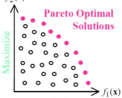
The complexity of solving multi-objective problems involves two types of problem difficulties: i) multiple, conflicting objectives, and ii) a highly complex search space. For instance, consider the following production planning example with two objectives, makespan (f1) and cost (f2), to be minimized under a set of constraints. For this bi-objective problem, an optimum design should ideally be a solution that achieves the minimum make span at a minimum cost without violating the constraints. If such a solution exists, then it is necessary to solve just a single-objective optimization problem, because the optimal solution for the first objective is also optimal for the second objective. However, this rarely happens in real life multi-objective problems. With multiple objectives, there is generally not one unique solution which is best (global minimum or maximum) with respect to all objectives but a set of solutions which can not be dominated by any other solutions in the search space. These solutions are known as Pareto optimal solutions or non dominated solutions (Chankong & Haimes 1983; Hans 1988).

Figure 1 : Pareto optimal solutions

This paper is focused on the post-Pareto optimality analysis. The two main objectives of the post-Pareto optimality analysis are: i) obtain a small sub-set of preferred solutions from the large

penalties are not required. The objective functions are ranked non-numerically based on their importance to the decision-maker, scaled and repeatedly combined into a single objective function using numerous randomly generated weight sets. The weight sets are selected to adhere to the decision maker’s objective function rankings. Then, the solution that gives the best result for a particular weight set is recorded. This process is repeated for a pre-selected number of iterations, and the final result obtained is a subset of solutions that most often provided the optimal combined objective function. This is a simple method that yields efficient results for any user who can prioritize the objective functions to find appropriate solutions.

In the second approach, we made use of clustering techniques used in data mining. In this case, we grouped the data by using the k-means algorithm to find groups of similar solutions, and since the solutions contained in each cluster are similar to one another, the decision-maker now has just k general solutions to choose from. In this later approach, the decision-maker is not required to specify any objective function preferences.

2. BACKGROUND

2.1 Multi-Objective Optimization Problems: A general

formulation of a multi-objective optimization problem consists of a number of objectives with inequality and/or equality constraints. Mathematically, the problem can be written as follows

minimize / maximize fi(x) for i = 1, 2, …,

n

g

(

x

)



0

h

(

x

)



0

x is an n dimensional vector having n decisions or variables. Solutions to a multi-objective optimization problem are mathematically expressed in terms of non dominated or superior points. It is useful to express non dominance in terms of vector comparison; let x and y be two

vectors of n components. Thus, x = (x1, x2,..,xn) and y = (y1, y2,..,yn).

for a maximization problem, that x dominates y, iff

for at least one i i {1,2,.., n}

similarly, for a

minimization

problem, that

x

dominates

y,

iff

and

x



y

for at least one i i {1,2,.., n}

X is defined as the set of feasible solutions or feasible decision alternatives. Thus, in a maximization problem x is

non dominated in X, if there exists no other in X such that

≥x and ≠x. The set of all non dominated solutions in X is designated N. Then, the optimal solutions to a

multi-objective optimization problem are in the set of non dominated solutions N, and they are usually known as the Pareto-optimal set.

2.2 Approaches to Solve Multi-Objective Optimization Problems: The two most common approaches to solve

multiple objective problems are: 1) combine them into a single objective function such as the weighted sum method or utility functions, or 2) obtain a set of non-dominated Pareto-optimal solutions. The weighted sum method belongs to the first approach. This method consists of aggregating all the objective functions together using different weighting coefficients for each one. This means that the multi-objective optimization problem is transformed into a single objective optimization problem. The problem can then be solved using a standard optimization algorithm or by using a heuristic.

Mathematically, the weighted sum formulation is written as:

Where

i



There is no real need or requirement for the wi terms to sum to one. However, this constraint is convenient and it is often added when the objective functions have all been similarly s

caled, e.g., 0 to 1. When the objective functions have been s

caled, the weights then represent the relative importance of each objective function. If the objective functions have not been scaled, then often the second, third, etc., objective functions have penalties assigned to them (for minimization problems). This is functionally identical to the weighted sum approach.

The weights must then be selected by the decision-maker prior to determination of the optimal solution. Often experienced practitioners have difficulty reliably selecting s

pecific values even if they are intimately familiar with the problem domain.

The solutions are strongly dependent on how the weights were chosen. Similarly, the choice of utility functions in utility theory is analogous to the selection of weights. In this case, a set of assumptions has to be made. For instance, it is often assumed that the different utilities are mutually independent, and either additive or multiplicative. Since utility theory is mathematically rigorous, more effort is needed to establish the utility functions.

I

n the second approach to solve multi-objective problems, optimization is conducted without the decision-maker articulating any preferences among the objectives. The outcome of this optimization is a set of Pareto-optimal s

olutions that reflects the trade-off between the objectives.

i



i i

y

x



) ( )

(

1

x f w x

f i

n

i i





1

0



w



1





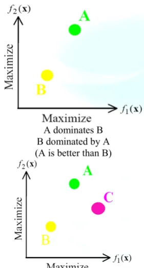
A dominates B B dominated by A (A is better than B)

A and C are non dominated with each other

This set can contain hundreds or even thousands of solutions, making it difficult for the decision maker to select one solution as final implementation. Then, there is a need to bridge the gap between single solutions and Pareto-optimal sets as shown in Figure 2.

Figure 2: Achieving a balance between single solutions and Pareto optimal solutions

Data Clustering:

In multi-dimensional situations, data clustering can be very insightful. Clustering is a data mining technique, which is used to solve classification problems. Currently, clustering methods are applied in many domains such as in artificial intelligence, pattern recognition, decision making and many more. Cluster analysis is used to find groups in data, and such groups are called clusters. Basically, the clusters are formed in such a way that objects in the same group are similar to each other, whereas objects in different groups are as dissimilar as possible.

There exists a wide variety of clustering algorithms. The two main branches of clustering algorithms are partitional and

hierarchical methods. The k-means algorithm is probably the most widely applied nonhierarchical clustering technique. The k-means algorithm is well known for its efficiency in clustering data sets. The grouping is done by calculating the centroid for each group, and assigning each observation to the group with the closest centroid. For the membership function, each data point belongs to its nearest center, forming a partition of the data. The objective function for the k-means algorithm is:

where,

i

x

j

c

This objective function gives an algorithm which minimizes the within-cluster variance (the squared distance between each center and its assigned data points). The membership function for k-means is:

   

 _

 



otherwise

j t ifl

x c

m_{KM l j} j

x

c

, 0

2 min

arg ,

1 ) |

(

||

||

The silhouette plot, to evaluate the quality of a clustering allocation, independently of the clustering technique that is used. The silhouette value for each point is a measure of how similar that point is to points in its own cluster compared to points in other clusters. It is defined as:

where, a(i) is the average distance from the ith point to all the other points in its cluster, and b(i) is the average distance from the ith point to all the points in the nearest neighbor cluster.

3. Combined Multiple Objective Genetic Algorithm (MOGA) and Post-Pareto Analysis:

The general approach involves the determination of a representative approximation of the Pareto optimal set using MOGAs, and then, filtering of that general set based on more specific information or decision maker input. We propose two methods to narrow the size of the Pareto optimal set, and thus, provide the decision-maker a workable size set of solutions, called the pruned Pareto set. The first method is called pruning by using non-numerical objective function ranking preferences and the second one is pruning by using data clustering.

When the decision-maker understands the objective function preferences to use but can not select specific wi values, he/she may prefer to use pruning by using the non-numerical objective function ranking preferences method, since this method will certainly provide solutions that reflect his/her

  i j n

i j k

c x C

X

KM 



1  1,..,

min )

, (





max

) ( ) ( ) (

i b i a

i a i b i

particular interests and priorities. On the other hand, if the decision-maker does not know a priori the importance of the objective functions, pruning by using data clustering is the most suited method to use. Moreover, the two methods can be sequentially combined in cases with larger number of objective functions.

3.1 Multiple Objectives Genetic Algorithm (MOGA) - NSGA

II

The first step is to determine an approximate Pareto optimal set using a MOGA. For our research, the fast elitist non-dominated sorting genetic algorithm II (NSGA-II) was proposed by

Deb et al. (2000a, 2000b). This algorithm is an improved version of the non dominated sorting genetic algorithm (NSGA). The algorithm reduces the computational complexity and maintains the solutions of the best Pareto front found including them into the next generation. This algorithm is highly efficient in obtaining good Pareto-optimal fronts for any number of objectives and can handle any number of constraints as well.

3.2 Pruning Using Non-numerical Objective Function

Ranking Preferences Method

This approach only requires the decision-maker to express his/her objective function Preference without having to provide exact weight values or specify utility functions. This is obviously, a rather soft way of stating information on priorities. Thus, the result of this method is a pruned Pareto set that clearly reflects the decision-maker objective function preferences.

Similar ideas have been explored in multiple criteria decision analysis. For example, Lahdelma et al., (1998) proposed Stochastic Multi objective Acceptability Analysis (SMAA) to explore the n-dimensional weight space based on an assumed utility function. In Rietveld and Ouwersloot (1992), a random sampling approach is proposed to generate quantitative values, which are consistent with the underlying ordinal information.

For other problem domains, similar pruning approaches have been used. For system reliability optimization problems, pruning has been demonstrated where the objectives were to maximize system reliability, minimize cost and weight (Kulturel-Konak et al, 2005; Taboada et al, 2005; Baheranwala, 2005; Coit & Baheranwala, 2005).

Initially, the objective functions are scaled, and then, ranked non-numerically by the decision-maker. Then, based on the rankings, an n-dimensional weight function fw(w) is

developed (similar to a joint distribution function), indicating the likelihood of different weight combinations. The algorithm used to prune Pareto-optimal solutions is listed below:

1. Rank objectives

2. Covert all objectives to be for maximization and Scale objectives (from 0 to 1)

3. Randomly generate weights based on ranks using the weight function fw(w)

4. Sum weighted objectives to form a single function f ′

5. From the Pareto optimal set, find the solution that yields the maximum (optimal) value for f ′

6. Increment the counter corresponding to that solution by a value of one

7. Repeat Steps 2 to 5 numerous (several thousand) times 8. Determine the pruned Pareto optimal set, i.e., the solutions that have non zero counter values

(counter > 0)

To demonstrate how this pruning method works, consider a problem with three objective functions.

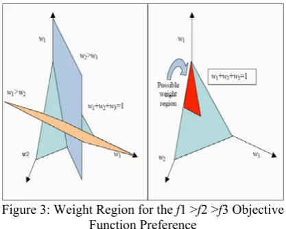
Consider the case where the objective function preference is f1 >f2 >f3, and thus, w1>w2>w3 for scaled objectives. For this region the weight function is defined as follows:

 

    

elsewhere w w w c w fw

, 0

, )

( 1 2 3

c is a constant so we are uniformly considering the possible weights within the preference region. Taking into account the decision-maker’s preferences, the region from where the weights are sampled and then combined with the objective functions, is shown in Figure3. A similar weight feasible region was described by Rietveld & Ouwersloot (1992).

Figure 3: Weight Region for the f1 >f2 >f3 Objective Function Preference

The weights, uniformly sampled from the region of interest, adhere to the decision maker’s objective function rankings. For instance, the possible values for the weights in the case f1>f2>f3 are 1/3w₁1,0w₂ 1/2and0w₃1/3.

The solution that gives the best result for this particular weight set is selected.

3.3 Pruning by Using Data Clustering

This approach is more useful for decision-makers that are less knowledgeable with the problem domain to specify any objective function preference. The result is a pruned Pareto set from which the decision-maker then only needs to consider k particular solutions.

Initially, the k-means clustering algorithm is used to group the solutions of the Pareto-optimal set into clusters. The k -means algorithm (MacQueen, 1967) is composed of the following steps:

1. Place k points into the space represented by the objects that are being clustered. These points represent initial group centroids.

2. Assign each object to the group that has the closest centroid.

3. When all objects have been assigned, recalculate the positions of the k centroids.

4. Repeat Steps 2 and 3 until the centroids stabilize (no longer move).

Like any clustering routine, which solves a minimization problem, k-means often converges to one of the many local minima, which is not necessarily the global solution. To overcome this situation, several runs are performed to find the smallest sum over all elements of the squared Euclidean distance (or another distance measure).

To determine the optimal number of clusters, k, we made use of the silhouette plot as suggested by Rousseeuw (1987, 1989). Since silhouette plots are based on the evaluation of the silhouette width, s(i), we calculated this measure for several values of k, and the clustering with the highest average silhouette width was selected as the optimal number of clusters in the Pareto optimal et.

After obtaining the optimal number of clusters, the data was grouped into k clusters. The members within a cluster are similar to one another, and members from one cluster to another are highly dissimilar. One approach to select a final solution, among all solutions contained in a group, is to identify what solution is the closest to its centroid. With this, the decision-maker has now just k general solutions to analyze, instead of all the solutions contained in the Pareto optimal set. Alternatively, the decision maker can first select the preferred cluster that most accurately reflects their priorities, and then, select from among those solutions within the cluster. If the solutions are indistinguishable or equivalent, then the solution closest to the centroid is again selected.

3.4 Combining the Non-numerical Objective Function Ranking Preferences Method and Data Clustering

The combination of the two proposed methods is ideally suited to address complex multi objective optimization problems in which the Pareto-optimal set is very large. For this type of problem, where the Pareto-optimal set can contain thousands of solutions, the combination of the two pruning methods might be preferred. In such cases, pruning by using the non-numerical objective function ranking preferences method should be initially applied to obtain a Pareto subset that reflects the decision-maker’s objective

function preference, and then, pruning by using data clustering can be applied to further reduce the size of the Pareto sub-set. Thus, the decision maker gets a smaller set of solutions to analyze and select one solution for implementation.

4. Numerical Example - Scheduling of Unrelated Parallel Machines:

An example is used to illustrate the two proposed methods to narrow the search space. The example addresses the scheduling of a Printed Wiring Board (PWB) manufacturing line (Yu et al., 2002). All analyses and computer runs were performed on personal computers. NSGA-II was compiled in C, and the data clustering was performed using MatLab. The drilling of PWBs is performed by a group of unrelated parallel machines (Yu et al.,2002) which must be scheduled. The processing time of each lot may be different for different machines, and a machine that has a shorter processing time for a particular lot may have a longer processing time for another lot. There are multiple criteria that need to be considered to determine the best schedule. Parallel machine scheduling problems are generally NP-hard problems (Karp, 1972). In terms of the complexity hierarchy of deterministic scheduling, unrelated machines scheduling problems are some of the most difficult to solve.

Yu et al. (2002) proposed a Lagrangian Relaxation Heuristic (LRH) method to solve this PWB scheduling problem. They constructed an integer programming model with a special structure called uni modularity. In order to account for multiple objectives of the scheduling system, they introduced preference constraints and brought them into the objective function by using Lagrangian relaxation.

We formulated the PWB scheduling problem as a multi-objective problem considering four multi-objectives to be minimized: minimize overtime, minimize average finish time, minimize the variance of the finish time and minimize the total cost. The multi-objective formulation is as follows:









i

C

m

C

x

o

1 1

1 1

2

_/

_,

_min

)

(

min

,

min

,

min





Subject to:





x

1





i

p

x

C

m

C

/







xij {0, 1} where,

Oi = overtime on machine i m = number of parallel machines n = number of lots to schedule

ij p = processing time of lot j on machine i ij c = cost of processing a lot j on machine i T = lot release interval time

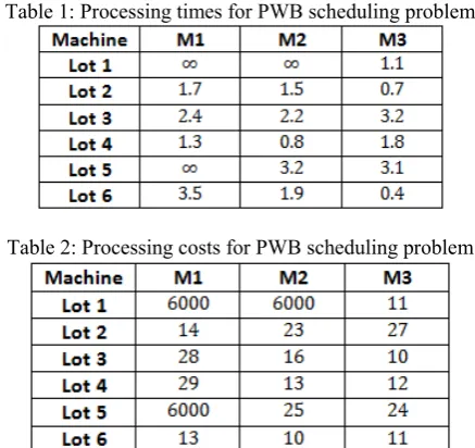
The processing times and the processing costs are shown in Tables 1 and 2 respectively (Yu et al, 2002). The release interval time, T, is equal to 3 time units. To satisfy feasibility, a large cost is assumed for processing a lot that cannot be processed by certain machines, such as in the cases of lot 1 on machine 1 and machine 2, forcing them to be scheduled on a machine that can perform the job.

Table 1: Processing times for PWB scheduling problem

Table 2: Processing costs for PWB scheduling problem

The multi-objective scheduling of this PWB problem was initially solved using the NSGA-II algorithm, to determine a Pareto optimal set; with a population size of 500 and the algorithm was run for 150 generations, with the probability of crossover as 0.7, and taking the probability of mutation to be 0.03. There were 28 solutions in the Pareto-optimal set. The post-Pareto analysis was then performed on these 28 solutions to provide the decision-maker a workable sub-set of solutions by using the two proposed methods.

4.1. Pruned Results Using the Non-numerical Ranking Preference Method:

The non-numerical ranking preference combination selected to illustrate this example is the case in which overtime (O) is more important than average finish time (AFT) , which is more important than variance of finish time (VFT), which is more important than cost (C) (O>AFT>VFT>C: w1>w2>w3>w4). Figure 4 shows, in a two-dimensional space, the 28 solutions contained in the Pareto-optimal set.

Figure 4: Pareto-optimal set in a two-dimensional space

Table 3 shows the pruned solutions obtained by applying the proposed method to narrow the search space. Of the original 28 solutions, the pruned set only includes 3; solution 1 has the minimum overtime but it is achieved at a higher cost than solutions 2 and 5. On the other hand, solution 5 presents the minimum cost but it has the highest average finish time as well as the highest variance of the average finish time.

Table 3 : Pruned solutions

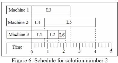
The pruned solutions obtained considering the w1>w2>w3>w4 objective function preference are shown in triangles in Figure 5. In this case, by using this method, it was achieved an 89.2% reduction in the solutions obtained from the Pareto-optimal set. These pruned solutions would then be further analyzed by the decision-maker. Solution 2 is shown as an example of a schedule for the PWB scheduling problem in Figure 6.

Figure 6: Schedule for solution number 2

4.1.2 Pruned Results by Using Data Clustering

Using the k-means algorithm, clustering analysis was performed on the 28 solutions contained in the Pareto-optimal set and we found k = 3 to be the optimal number of clusters with the aid of the silhouette plots. Figure 7 shows the three clusters in a three-dimensional space, for minimizing overtime, minimizing average finish time and minimizing cost. Figure 8 shows the clusters in a three-dimensional space for minimizing overtime, minimizing average finish time and minimizing the variance of the average finish time. In Figures 7 and 8, the fourth objective (minimize variance of average finish time and minimize cost, respectively) is not shown but it is still considered in the analysis. The objective functions have been scaled from 0 to 1.

Figure 7: Clustered data in a three-dimensional space

Figure 8 Clustered data in a three-dimensional space

Table 4 shows the summary of the results obtained by using the k-means algorithm. This table includes the representative solutions that were closest to their corresponding centroid. As we can see from Table 4, solution number 6 from cluster 2 gives the minimum overtime, average finish time and

variance of the average finish time but it has the highest cost. On the other hand, solution 28 from cluster 1 has the lowest cost but it also gives the highest overtime and variance of the average finish time. The decision-maker has to pick one solution; in this case solution 6 from cluster 2 may seem to be the most promising solution since it achieves the minimum value in 3 out of the 4 objective functions considered. Figure 9 shows the schedule for solution 6.

Table 4: Results obtained with the cluster analysis

Figure 9: Schedule for solution number 6

For both pruning methods, the decision-maker only needs to consider three solutions (instead of 28). It is much easier and convenient to select from among 3. The first pruning method is most appropriate when the decision-maker can prioritize their objectives, while the second does not require the decision-maker to a priori specify any objective function preference.

V. CONCLUSION

A popular method of “solving” multi-objective problems is to determine a Pareto-optimal set or sub-set. However, this then requires the decision-maker to select from among this set of solutions, which is often large when there is more than two objective functions. Therefore, meaningful research has to be done to support the decision-maker during this post-Pareto analysis phase. In this paper, two methods are reviewed to prune the size of the Pareto-optimal set. This pruned Pareto set gives the decision-maker a workable sized set of alternatives to choose from.

using the weight function fw(w) which reflects the

decision-maker preferences.

In the second approach, we used the k-means algorithm to group the solutions of the pareto optimal set into k different clusters, and since members in the same cluster are similar to each other, the solution that was closest to the centroid of each cluster was chosen to be the representative solution in its respective cluster. Then, the size of the Pareto-optimal set was reduced to just k general solutions to analyze by the decision-maker.

The two methods were demonstrated on the scheduling of the bottleneck operation of a PWB manufacturing line. In general, the two proposed methods are approaches that help achieve a continuum between Pareto-optimal solution sets and single solutions.

REFERENCES

1. Baheranwala, F. Solution of Stochastic Multi-objective Combinatorial problems. MS thesis,2005. Rutgers University, USA.

2. Chanking, V. and Haimes, Y. (1983). Multiobjective decision making theory and methodology. New York: North-Holland.

3. Coit, D.W and Baheranwala F. Solution of Stochastic Multi-objective System Reliability Design Problems Using Genetic Algorithms.

Proceedings of the European Safety and Reliability Conference

(ESREL), Gdansk, Poland, June 2005

4. Deb, K., Pratap, A., Agarwal, S. and Meyarivan, T. (2000). A Fast and Elitist Multi-Objective Genetic Algorithm-NSGA-II. KanGAL Report Number 2000001.

5. Hans, A.E. (1988). Multicriteria optimization for highly accurate systems.

Multicriteria Optimization in Engineering and Sciences. W.Stadler (Ed.), Mathematical concepts and methods in science and engineering,

19, 309-352.

6. Karp, R.M. (1972) Reducibility among combinatorial problems, in Complexity of Computer Computations, Miller, R.E. and Thatcher, J.W. (eds.), Plenum Press, New York. 85– 103.

7. Kaufman L. and Rousseeuw P.J. (1990). Finding groups in data. An introduction to Cluster Analysis. Wiley-Interscience.

8. Korhonen P. and Halme M. (1990). Supporting the decision maker to find the most preferred solutions for a MOLP-problem. Proceedings of the 9th International Conference on Multiple Criteria Decision Making. Fairfax, Virginia, USA, 173-183.

9. MacQueen J. (1967): Some methods for classification and analysis of multivariate observations. In L. M. LeCam and J. Neyman, editors,

Proceedings of the Fifth Berkeley Symposium on Mathematical Statistics and Probability, 1, 281–297.

10. Mohan, S. and Raipure, D. M. (1992). Multiobjective Analysis of Multireservoir System. Journal of Water resource Planning and management, 118(4), .356-370.

11. Raipure, D.M. (1990). Multiobjective analysis of reservoir system, M. Tech. Thesis, Indian Institute of Technology, Madras, India.

12. Rao, S.S. (1991). Optimization theory and application. New Delhi: Wiley Eastern Limited.

13. Rousseeuw Peter J. (1987): Silhouettes: A graphical aid to the interpretation and validation of cluster analysis. Journal of computational and applied mathematics, 20, 53-65.

14. Rousseeuw P., Trauwaert E. and Kaufman L. (1989): Some silhouette-based graphics for clustering interpretation. Belgian Journal of Operations Research, Statistics and ComputerScience, 29(3).

15. Shie-Yui L., Al-Fayyaz T. and Kim Sai L. (2004). Application of Evolutionary Algorithm in Reservoir Operations. Journal of The Institution of Engineers, Singapore, 44(1), 39-54.

16. Venkat V., Jacobson S. and Stori J. (2004). A post-Optimality Analysis Algorithm for Multi- Objective Optimization. Computational Optimization and Applications, 28, 357-372.

17. Yu Lian, Shih H.M, Pfund M., Carlyle W.M. and Fowler J.W. (2002). Scheduling of Unrelated Parallel Machines: an Application to PWB manufacturing. IIE Transactions, 34,921-931.

18. Zeleny, M. (1982). Multiple Criteria Decision Making. McGraw-Hill series in Quantitative Methods for Management.

AUTHORS BIOGRAPHY

Praveen Kumar Malladi is pursuing M.Tech in Software Engineering

from GITAM UNIVERSITY, Visakhapatnam, A.P., INDIA. My research areas include Software Reliability, Software Quality and Software Cost Estimation Techniques.

Deepika Puvvula is pursuing M.Tech in Software Engineering from GITAM UNIVERSITY, Visakhapatnam, A.P., INDIA. Her research areas include Software Quality Assurance, Software Reliability and Software Cost Estimation Techniques.

Anisha Nagalla is pursuing M.Tech in Software Engineering from GITAM