Theses Thesis/Dissertation Collections
9-2014
A Brain Computer Interface for Interactive and
Intelligent Image Search and Retrieval
Shitij P. Kumar
Follow this and additional works at:http://scholarworks.rit.edu/theses
This Thesis is brought to you for free and open access by the Thesis/Dissertation Collections at RIT Scholar Works. It has been accepted for inclusion in Theses by an authorized administrator of RIT Scholar Works. For more information, please [email protected].
Recommended Citation
A Brain Computer Interface for Interactive and
Intelligent Image Search and Retrieval
by
Shitij P. Kumar
A Thesis Submitted in Partial Fulfillment of the Requirements for the Degree of Master of Science
in Electrical and Microelectronic Engineering Supervised by
Professor Dr. Ferat Sahin
Department of Electrical and Microelectronic Engineering Kate Gleason College of Engineering
Rochester Institute of Technology Rochester, New York
September 2014
Approved by:
Dr. Ferat Sahin, Professor
Thesis Advisor, Department of Electrical and Microelectronic Engineering
Dr. Gill Tsouri, Associate Professor
Committee Member, Department of Electrical and Microelectronic Engineering
Dr. Sildomar T. Monteiro , Assistant Professor
Committee Member, Department of Electrical and Microelectronic Engineering
Dr. Sohail A. Dianat , Professor
Thesis Release Permission Form
Rochester Institute of Technology Kate Gleason College of Engineering
Title:
A Brain Computer Interface for Interactive and Intelligent Image Search and Retrieval
I, Shitij P. Kumar, hereby grant permission to the Wallace Memorial Library to repro-duce my thesis in whole or part.
Shitij P. Kumar
Dedication
I dedicate this work to my loving family who has supported and inspired me in everything that I have done, to my closest of friends who have helped and motivated me, my teachers and mentors who have never failed to guide and inspire me and most of all the ’Big Boss
Acknowledgments
Through my years here, there are many I would like to thank.
Above all, I am grateful for the guidance and generosity, that has and continues to be provided by my advisor Dr. Ferat Sahin. His words of inspiration and wisdom have found
themselves contributing to the basis of my success.
I would like to convey special thanks to Rochester Institute of Technology for the Effective Access Technologies Grant for this work.
I am grateful to all my peers and fellow research assistants at the Multi-Agent Biorobotics Laboratory. Each of you have contributed your unique roles in the completion of this
work.
Ryan, thank you for being an excellent mentor and a great friend. The software architecture of this work was only possible because of your guidance, thanks. Eyup, it was your initial work and help during the Bio-Robotics Class that inspired this
work, thanks.
Dan, our discussions about the human-behavior were very helpful while designing the user interface of the proposed Brain Computer Interface, thanks.
Abstract
A Brain Computer Interface for Interactive and Intelligent Image Search and Retrieval
Shitij P. Kumar
Supervising Professor: Dr. Ferat Sahin
This research proposes a Brain Computer Interface as an interactive and intelligent Image Search and Retrieval tool that allows users, disabled or otherwise to browse and search for images using brain signals. The proposed BCI system implements decoding the brain state by using a non-invasive electroencephalography (EEG) signals, in combination with machine learning, artificial intelligence and automatic content and similarity analysis of images. The user can spell search queries using a mental typewriter (Hex-O-Speller), and the resulting images from the web search are shown to the user as a Rapid Serial Visual Presentations (RSVP). For each image shown, the EEG response is used by the system to recognize the user’s interests and narrow down the search results. In addition, it also adds more descriptive terms to the search query, and retrieves more specific image search results and repeats the process. As a proof of concept, a prototype system was designed and implemented to test the navigation through the interface and the Hex-o-Speller using an event-related potential(ERP) detection and classification system.
List of Contributions
• Design of a software architecture for the proposed Brain Computer Interface. Gen-eration of visual stimuli like the Hex-O-Speller, rapid Serial Visual Presentation for the proposed Brain Computer Interface and other Hex-O-Speller based stimuli, but instead of characters other information is shown.
• Development of an automated stimulus generation and data collection system for the proposed Brain Computer Interface.
• Comparison of results from the Event Related Potential detection and classification system developed for the proposed BCI, bu using three different Feature Extraction Methods : Band Powers, Time Segments and Wavelet Decomposition in combina-tion with four different classification methods: Linear Discriminant Analysis (LDA), optimized LDA, Support Vector Machine (SVM) and Neural Networks (NN).
• Publication
Contents
Dedication . . . iii
Acknowledgments . . . iv
Abstract. . . v
List of Contributions. . . vii
1 Introduction . . . 1
2 Background Literature . . . 4
2.1 Stimulus Generation . . . 5
2.1.1 P300-Matrix Speller . . . 6
2.1.2 Hex-O-Speller . . . 7
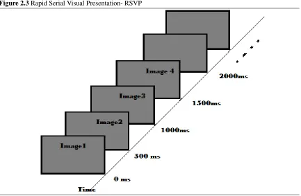
2.1.3 Rapid Serial Visual Presentation . . . 7
2.1.4 Psychtoolbox 3.0 . . . 7
2.2 Data Collection and Other Analysis Tools . . . 9
2.2.1 Basic structure of a Human Brain . . . 9
2.2.2 Electrode Placements and Data Collection Hardware . . . 11
2.3 Pre-processing of EEG signals . . . 13
2.3.1 Filtering . . . 14
2.3.2 Artifact Removal . . . 15
2.3.3 Pre-processing of the Corrected Artifact Free Data . . . 18
2.3.4 Feature Extraction Methods . . . 20
3 Proposed Method . . . 25
3.1 View . . . 26
3.1.1 Training . . . 27
3.1.2 Navigation . . . 27
3.1.3 Hex-O-Speller . . . 27
3.2 Model . . . 27
3.2.1 Motor Imaginary Movement Algorithm . . . 28
3.2.2 ERP Detection Algorithm . . . 28
3.2.3 ERP Yes/No Algorithm . . . 29
3.2.4 ERP Score Generation Algorithm . . . 29
3.2.5 Content Based Image Similarity Map Generation Algorithm . . . . 29
3.2.6 Image Queuing/Ranking and Search Query Refinement Algorithm . 29 3.3 Controller . . . 30
3.3.1 Data Collection, Organization and Timing Synchronization during Visual Stimulus . . . 30
3.4 ERP Detection System and the Yes/No (2-Class Target/non-Target) Classifier 35 4 Results . . . 40
4.1 Results of the ERP Detection and Classification on a Standard Dataset . . . 40
4.1.1 Data Description and Protocol . . . 41
4.1.2 Pre-processing: Results of ICA Correction . . . 43
4.1.3 Pre-processing: Spatial and Temporal Selection . . . 43
4.1.4 Comparison of Results for ERP detection . . . 45
4.2 Results from the Prototype BCI System . . . 46
4.2.1 Experiment Methodology and Setup . . . 48
4.2.2 Results of Simultaneous Data Collection and Stimulus Generation . 49 5 Conclusions . . . 60
6 Future Work . . . 62
Bibliography . . . 64
A Topographic map of an EEG field as a 2-D circular view . . . 68
B Receiver Operating Characteristic (ROC) Plots . . . 75
List of Tables
4.1 Independent Components Rejected for Subject A and Subject B . . . 43 4.2 Channels Selected for Subject A and Subject B . . . 44 4.3 Time Segments Selected for Subject A and Subject B(from 1 to 168 data
points i.e. 0.7 seconds) . . . 45 4.4 Result Comparison for p300 Matrix speller Dataset for different Feature
List of Figures
2.1 P300-Matrix Speller [1] . . . 6
2.2 Hex-O-Speller - Steps 1 and 2 showing the selection of the character ’A’ [2] 7 2.3 Rapid Serial Visual Presentation- RSVP . . . 8
2.4 The Human Brain-Cerebrum [3] . . . 12
2.5 EEG Electrode Placement 10-20 System [1] . . . 13
2.6 20 channel EEG Electrode Placement [4] . . . 14
2.7 Raw signal and its Power Spectrum depicting the DC offset noise and 60 Hz noise in a Channel (screen shot from the Bio-Capture Software) [5] . . . 15
2.8 ICA decomposition [6] . . . 17
2.9 Summed Projection of Selected Components [6] . . . 18
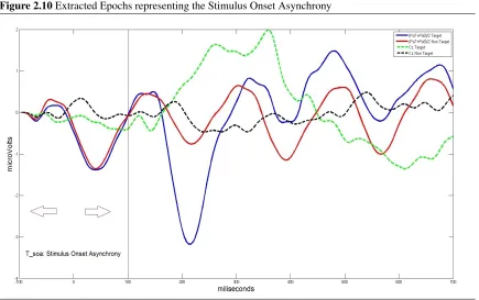
2.10 Extracted Epochs representing the Stimulus Onset Asynchrony . . . 19
2.11 Time Interval Windows Selected based upon signed−r2values . . . 23
3.1 Proposed Approach Block Diagram [2] . . . 26
3.2 Data Collection System Block Diagram . . . 36
3.3 Timing Diagram . . . 37
3.4 Block Diagram of the ERP Detection and Classification System . . . 38
4.1 ERPs in the P300 Matrix Speller Dataset for Subject A and Subject B (in that order) in the mean signal across all data samples/epochs for target and non-target stimuli. . . 42
4.2 Spatial Selection for Subject A . . . 52
4.3 Spatial Selection for Subject B. . . 53
4.4 Topographic map of BD as a 2-D circular view for Subject A and B . . . . 54
4.5 Temporal Selection for Subject A . . . 55
4.6 Temporal Selection for Subject B . . . 56
4.7 Examples of Training Visual Stimuli . . . 57
4.8 Sample Raw Data window and Epoch Extraction of a Single channel . . . . 58
4.9 ERPs in the BCI for self-collected data in the mean signal across all data samples/epochs for target and non-target stimuli. . . 59
Chapter 1
Introduction
A
ssistive devices and technologies are essential in enhancing the quality of life for indi-viduals. A lot of research in developing assistive smart devices and technologies for disable individuals that depend on motor movements, speech, touch and bio-signals has been done. Most of these systems for disabled individuals depend on some residual motor movement or speech.Whereas the BCI systems completely bypass any motor-output by decoding the Brain state of an individual, which can be an emotion, attention i.e. an event related poten-tial (ERP) or an imagined movement [7][8][9][10][11]. These can help disabled individuals that have almost none to some voluntary muscle/movement control, thereby attempting to give some autonomy to individuals by providing the brain with alternate ways of commu-nication. Significant EEG based researches that try to classify and understand various brain states like movement of limbs, imaginary or otherwise, emotions, attention etc. have been done but very few have tried to combine and decode these brain states and apply them in daily used applications like a web search.devices, computers and applications especially the ones that use the information available on internet are indisputable. The users expect the applications and technologies to be smart and learn from the usage and the choices made by the user. The proposed study will further reinforce this notion, by taking into consideration and understanding their thoughts/actions by decoding their brain state, thus making them more user friendly and intelligent. A lot of studies in the psychophysiology and neuroscience fields have been done to understand the relation of emotions, attention, interest, motor movements etc. to the Brain activity and EEG responses [12][13][14][15][16][17][18][9]. But there are relatively fewer real world applications that use these researches.
similar freedom and autonomy as the other capable general population.
The principal challenge with this research is that there is no defined model or relation that relates a user’s interest to the contents of an image. In order to formulate a relation, experiments as proposed in Chapter 6 and [2] can be designed and performed using the proposed BCI. Another challenge is that a large amount of training data is needed to be collected, thereby a longer training time, for getting higher accuracy for a single-trial EEG signal classification [7][8]. Also the EEG recording devices are a bit uncomfortable and less fashionable. However, there have been significant advances in wearable technologies and new devices like the Emotive research headset [22], EEG head bands etc. that collect wireless EEG data are relatively comfortable and fashionable. Nonetheless, this study is step towards better understanding the use of Bio-Signals as a feedback to devices and ap-plications to understand the user better.
Chapter 2
Background Literature
Understanding the brain function is a challenge that has inspired a lot of research and insight from researchers and scientists from multiple disciplines. This resulted in the emer-gence of computational neuroscience, the principle theoretical approach in understanding the workings the nervous system [7]. Part of this research involves decoding the brain-state/human intentions by using the the EEG(electroencephalogram) signals. This branch of the field is greatly influenced by the development of effective communication interfaces connecting the human-brain and the computer [7]. This chapter describes the research, studies and other similar brain-computer interfaces that have been used as a reference and guide for this work.
stored corresponding to the event that evoked it. Thus the setup and collection of the EEG data is the second step in the development of a BCI. The first two steps occur concurrently, hence synchronization and timing is a crucial part for effecting data collection. Thirdly, the pre-processing and representation of the EEG data. For effective representation of EEG data, the data is cleaned and is represented by a reduced subset of features. The last step in-volves generation of models that can classify the EEG signals representing different events. Once the EEG response to an event is classified/identified, subsequent action based on the purpose of the BCI can be taken.
2.1
Stimulus Generation
Generally every Brain Computer Interface requires a medium of communication repre-sented by an event that evokes an EEG response. This event can be of the type visual, muscle movement, auditory or touch. Here in this research a visual event is used to gener-ate an EEG response.
The most commonly researched example of this stimulus is the attention based mental typewriter. This mental typewriter is used to spell words using the EEG signals. The following subsection explains the visual stimuli used in this research.
2.1.1 P300-Matrix Speller
[image:19.612.96.524.399.620.2]The so called Matrix Speller consists of a 6x6 character matrix as shown in Figure 2.1 where in characters are arranged within rows and columns [1]. throughout the stimulus generation process the rows and columns are intensified (’flashed’) in a random order one after the other. The subject is asked to focuses on the targeted character for the span of stimulus and EEG response corresponding to each intensification is recorded. As the EEG response can be modulated by attention, the response for the targeted character is different from the non-target characters.
2.1.2 Hex-O-Speller
The Hex-O-Speller is a variant of the Matrix speller [7]. It is represented with six circles placed at the corners of an invisible hexagon as shown in Figure 2.2. Each circle is inten-sified (’flashed’) in a random order multiple times. Intensification is realized by up-sizing the circles by 40 percentfor 100milliseconds. In this speller the choice is made in two re-current steps. At the first step, the group containing the target symbol/character is selected, followed by the selection of the target symbol itself at the second step.
Figure 2.2Hex-O-Speller - Steps 1 and 2 showing the selection of the character ’A’ [2]
2.1.3 Rapid Serial Visual Presentation
Rapid Serial Visual Presentation (RSVP) is an experimental setup used to understand tem-poral characteristics of attention. In this setup images are flashed or shown for a fixed duration at specific intervals as show in Figure 2.3.
2.1.4 Psychtoolbox 3.0
Figure 2.3Rapid Serial Visual Presentation- RSVP
RSVP are generated using the Psychtoolbox. It allows control and flexibility to record the time for events which helps generate decently accurate event markers necessary for data segmentation(epoching or shelfing). Every display screen has a display buffer and a ’Vertical Blank Interval’ time [25] also know as V − Blank, that it takes to completely display a new image. This toolbox gives a two stage flexibility to change a display on a monitor. The first step is filing the display buffer with the desired image and second is ’Flipping’ the screen i.e. clearing the previous display and showing the new display. The refresh rate of a monitor depends on the type of monitor, operating system and the graphics card. This rate remains the same for the stimulus running on a specific system. This refresh rate sayTre f resh, becomes the unit time for change of display on a monitor.
image. TheV−Blankinterval is represented asV−Blank=n∗Tre f eresh, wherenbeing the
time taken to show the image in the image buffer onto the screen in unitsTre f resh. For all
images to be displayed thisV−Blanktime can be fixed to the maximum possible time taken for the biggest image to be displayed during the stimulus. This results in a uniform screen change rate, thus making the synchronization of stimulus generation and data collection better.
2.2
Data Collection and Other Analysis Tools
Data collection is an integral part of any Brain Computer Interface. Data collection requires proper setup of electrodes and bio-signal collection devices. These devices generally con-tain buffers and amplifiers to amplify the bio-signal data and transmit it to the computer. It is extremely important for proper synchronization between stimulus generation for the event that evokes the EEG response and its collection, to correctly segregate (also known as epoching or shelving) the EEG response corresponding to the event. An implementation of the simultaneous data collection and stimulus generation tool for the proposed BCI is discussed in detail in Chapter 3.
2.2.1 Basic structure of a Human Brain
medulla are referred to together as the brainstem. Here, the part where the EEG signals are collected from is know as the Cerebrum. The cerebrum or cortex is the largest part of the human brain, associated with higher brain function such as thought and action. The cerebral cortex is divided into four sections, called ”lobes”: the frontal lobe, parietal lobe, occipital lobe, and temporal lobe. The visual representation of the cortex is shown in Figure 2.4. Each lobe of the brain has a specific function.
• Frontal Lobe is associated with reasoning, planning, parts of speech, movement, emotions and problem solving.
• Parietal Lobeis associated with movement, orientation, recognition and perception of stimuli.
• Occipital Lobeis associated with visual processing.
• Temporal Lobe is associated with perception and recognition of auditory stimuli, memory and speech.
The EEG signals or brain waves have specific bands of frequencies that are most active corresponding to a brain state. As explained in [26] EEG has four main bands delta(δ),
theta(θ),alpha(α) andbeta(β).
– beta(β1) brainwaves (13-15 Hz) are associated with being in a physically relaxed
and mentally alert state of mind. These waves are often associated with peak performance training, e.g., professional athletes.
– beta(β2) brainwaves (16-18 Hz) are typically associated with performing mental
tasks such as reading, mathematics and problem solving.
– beta(β3) brainwaves (19-26 Hz) are also associated with problem solving and
thinking in general, however, there is also some association with worry or anxiety.
• alpha(α) waves are slower, larger brainwaves (8 Hz - 12 Hz) than the beta waves and are associated with the state of relaxation. Their presence represents the brain in a relaxed, somewhat disengaged state, waiting to respond if needed.
• theta(θ) brainwaves (4 Hz - 8 Hz) represent a daydream-like, rather spacey state of mind that is associated with mental inefficiency. At very slow levels, theta wave ac-tivity is associated with a very relaxed state and often represents the twilight zone between wakefulness and sleep.
• delta(δ) brainwaves (.50 Hz - 3.5 Hz) are the slowest, highest amplitude (magnitude) brainwaves, and are what a person experiences when asleep.
2.2.2 Electrode Placements and Data Collection Hardware
Figure 2.4The Human Brain-Cerebrum [3]
have 14 channels, and some headbands have only four. For this work an EEG cap with 20 channels is used. Figure 2.6 shows the placement of electrodes. These electrodes through cable are connected to data-collection hardware that generally have two-stage amplifiers as the magnitude of EEG signals ranges in micro volts along with analog-to-digital converters. There are various data-collection hardware available such as Bio-Radio 150 [5], Bio-Semi [27], B-Alert[28], Emotive head set [22] that collect the data. Here Bio-radio 150 is used. According to the bio-radio manual [5], the data is collected and wirelessly transmitted via blue-tooth in serialized data packets. The Bio-Radio 150 provides libraries so that its functions can be called and the data collected parsed and put into a proper matrix
• Xbioradio of dimensions (cx p) where c is the Number Of Channels/electrodes
Figure 2.5EEG Electrode Placement 10-20 System [1]
channel/electrode.
It also allows the system to configure the data sampling rate and resolution of the data collected. A maximum of eight channels can be connected to a single Bio-radio 150. As more than 8 channels are required for getting sufficient information to represent an Event Related Potential (ERP), programs for recording EEG signals from multiple Bio-Radio 150 modules simultaneously are implemented.
2.3
Pre-processing of EEG signals
Figure 2.620 channel EEG Electrode Placement [4]
movement and blink artifacts i.e. Electrooculogram (EOG) (if they are not considered as useful information for the objective of the Brain Computer Interface classification), Elec-trocardiogram (ECG) noise, and other muscle movement noise (voluntary or involuntary).
2.3.1 Filtering
Instrument noise present in the raw signal can be either because of the 60 Hz power noise , noise over the wireless communication or if the electrode cable is not connected properly to the Bio-radio 150 (see Figure 2.7). As described in Section 2.2 the main bands of EEG signal generally range from 0.5 Hz to 30 Hz. In order to remove the DC noise and the 60 Hz noise, the raw signal can be filtered using a band-pass filter. Here in this work a 6th order Butterworth band pass filter with cut-offfrequencies as 0.1 Hz and 30 Hz is used [8].
Figure 2.7Raw signal and its Power Spectrum depicting the DC offset noise and 60 Hz noise in a Channel
(screen shot from the Bio-Capture Software) [5]
2.3.2 Artifact Removal
the effects of large amplitude outliers which are representative of these artifacts. In [8] this method is used to dampen the effects of these artifacts. Both methods are described briefly below:
Independent Component Analysis (ICA)
ICA based artifact correction can separate and remove wide variety of artifacts from EEG data by linear decomposition. However, there are certain assumptions that are made [6][29]. They are :
• (1) : spatially stable mixtures of activities of temporally independent brain and arti-fact sources
• (2) : summation of potentials from different channels/sensors is linear at the elec-trodes
• (3) : propagation delays from the source of the electrodes is negligible For analyzing the EEG signals, letXbe the input response matrix where
• X of dimensions (N x P), whereN is the number of channels and Pis the number of data points.
The ICA finds an unmixing matrix W which linearly decomposes the multi-channel EEG data into sum of temporally independent and spatially fixed components.
U = W·X (2.1)
at each electrode. Columns of W−1 are used to determine which components are to be selected. Say a set ofacomponents are selected, then clean data can be represented as
CleanData =W−1(:,a)∗U(a,:) (2.2) , where the dimensions of each matrices are
• CleanData: (cxN)
• W−1(:,a) : (cx length ofa) • U(a,:) : (length ofaxN)
[image:30.612.94.525.385.607.2]Figures 2.8 and Figure 2.9 show the decomposition and summed projection of the selected ICA components as decribed in [6].
Figure 2.8ICA decomposition [6]
Winsorizing Data- Clipping
Figure 2.9Summed Projection of Selected Components [6]
the first and last (0.5∗p)thpercentile of the sorted values of the data vector are replaced by
the value nearest to the side of the sorting order.
For a sorted data vector say X = X1,X2,X3,X4,X5, ..,X99,X100, 10th percentile
win-sorizing will results inXclipped=X6,X6,X6,X6,X6,X6,X7, ...X93,X94,X94,X94,X94,X94,X94,
whereXandXclipped have the same length.
2.3.3 Pre-processing of the Corrected Artifact Free Data
The corrected data is segmented (epoched/shelved) corresponding to the response of each stimulus. In order to keep the ratio of meaningful signal to that of noise high, multiple trials of the same stimulus are performed and data collected. These trials are averaged in order to attenuate the noise. Each data sample has data points corresponding to time interval TS OA
prior to the display of the stimulus and data points after the display of the stimulus. This signal collected for the time interval TS OA is called Stimulus Onset Asynchrony (SOA).
rest of the data sample. This is called ’Baseline Correction’. As the data collection for a stimulus is continuous during a trial baseline correction is very important to remove any change of offset due to the response to the previous stimulus in a trial.
[image:32.612.94.529.339.612.2]Following the guidelines of recording EEG signals and ERP data as given in [30], the EEG signal data is re-referenced and baseline corrected. Re-referncing EEG data means that reference channels are to be subtracted from all other channels. Generally the reference channels selected are the signals from mastoids i.e. Channels A1 and A2 as shown in 2.6. Another re-referencing method used is subtracting the mean of all channels at a given data point from all the channels. Here the later is used as the re-referencing procedure.
2.3.4 Feature Extraction Methods
After the raw EEG data is corrected, segmented/epoched, re-referenced, averaged and base-line corrected feature extraction is performed. Here event-related potentials (ERPs) in the collected EEG signals are to be identified and classified. The property of an ERP lies in both spatial and temporal domain. Spatial domain is the representation of the signal generated at different channels( electrodes/sensors) and the contribution of each channel to successfully characterize an ERP. Temporal domain represents the generation of ERP after the stimulus is shown. This response time varies from subject to subject. Some subjects might respond faster or slower than other subjects. However, it has been noted that for an average per-son the ERP response, specifically the P-300 response happens 300 milliseconds after the stimulus event occurs [1][8]. Hence the nomenclature of P-300 Matrix Speller, as it tries to identify this specific data point response in an EEG response to a stimulus.
Spatial- Channel Selection
target patterns. This real-valued scalerBDcan be defined as:
BD= 1
8(m1−m2)
TC1+C2
2
−1
(m1−m2)+
1 2ln
| C1+C2
2 |
√
|C1 | ∗ |C2 |
(2.3) where |˙ | denotes the determinant of a matrix, m1 is the mean vector of target pattern
signals, m2 is the mean vector of non target pattern signals, andC1 andC2 are the
corre-sponding co-variance matrices. Results of using this statistical measure on the standard dataset provided in [1] are shown in Chapter 4.
Temporal- Time Intervals/Window Selection
Similar to the spatial selection certain time intervals in the EEG response from each se-lected channels contain more discriminative information for target patterns and non target patterns. This approach is used in [7] to select clusters of timing data points for generation of features. The statistical measure used in [7] is a biserial correlation coefficient r. This correlation coefficient is defined as
r(x)=
√
N1∗N2
N1+N2
!
mean(xi |yi = target)−mean(xi |yi = non−target)
std(xi)
!
(2.4) where N1 and N2 are the number of samples for target and non− target patterns, xi is
the data point in the time series at time ti of the signal for a selected channel , yi is the
classification of the pattern i.e. either targetor non−target, mean(.) is the mean of the vector of the data points across samples and std(.) is the standard deviation of the vector of data points across all samples,targetandnon−target. The discriminative measure used is
signed−r2 value which is
Results of using this statistical measure on the standard dataset provided in [1] are shown in Chapter 4.
Following the identification of discriminative spatial channels and temporal data points, features representing them can be generated. The temporal characteristics of the EEG signal can be identified and represented, both in time and frequency domain. Here in this research three different methods for feature selection were used for comparison.
Band Powers: Sum of Fast Fourier Transform(FFT) Coefficients for specific EEG bands
This feature extraction method explores the frequency domain features of the signal. For each channel of an EEG response the signal is passed though various band-pass filters with cut-offfrequencies representing different bands of the EEG signal (Section 2.2.1) and the corresponding FFT is taken and the absolute values of the FFT coefficients are used to represent each channel. These coefficients are summed at fixed equally spaced intervals and vectorized to represent a feature vector for all channels.
Procedure 2.1FFT Feature Extaraction
Input:data Samplexi
Input:cut-offfrequencies for EEG bands
Input:Sampling Rate of Data Collection
Output: Feature Vector Representing thexi
Sum of Timing Segments/Windows
• xi of dimensions (c x p) for i ∈ [1,N1 + N2], where c is the Number of selected
channels and p is the Number of data points in the signal and N1 and N2 are the
number of samples in the target and non-target pattern signals respectively.
• Let τi jk represent a set of time interval where j ∈ [1,c] and k ∈ [1,m], and m is
the Number of Time Intervals identified. Figure 2.11 shows an example of timing intervals being selected.
• LetX be the feature set representingx. Then Xi =
n
Xi jk∀j∈[1,c],k∈[1,m]
o
, where
Xi jkis the sum of all data points in the time intervalτi jkfor channel jof data samplei. • Xi jk = Pτkxi j, where xi j is the signal of data samplei ∈ [1,N1 +N2] from channel
[image:36.612.96.526.399.694.2]j∈[1,c], andτk is thekth∈[1,m] time interval.
Wavelet Decomposition
Chapter 3
Proposed Method
Figure 3.1Proposed Approach Block Diagram [2]
interest the user have been identified, the user can choose the image or sub-set of images that he/she likes the most.
The proposed BCI system is modeled as a Model View Controller (MVC) architecture as shown in Figure 3.1. The working of the system is described in detail as follows:
3.1
View
Navigation, Hex-O-Speller and RSVP. Their function is explained in detail below.
3.1.1 Training
The Training generates different visual stimuli for ERP detection, motor imaginary move-ments and eye movemove-ments during the training of the system for a specific user.
3.1.2 Navigation
The Navigation displays different options for easy navigation through the interface either by using ERP detection or through motor imaginary movements.
3.1.3 Hex-O-Speller
The Hex-O-Speller is used to type search queries which are then passed to the Controller for image retrieval from the web (see Section 2.1.2).
3.1.4 RSVP-Rapid Serial Visual Presentation
After the images are retrieved and processed these images are shown to the user in a rapid serial visual presentation (RSVP) (see Section 2.1.3).
The stimulus generator handles the change and the placement of proper information in all of these displays.The rate of change and timing of the visual stimulus is synchronized with the Controller (Section 3.3). The Stimulus Generator also provides the necessary information about the visual stimulus to the Controller for tracking and organizing the data representing the EEG response corresponding to the visual stimulus.
3.2
Model
generator to change and update the display based on the EEG response corresponding to the previous stimuli. The model contains sub-systems for classifying motor imaginary movements, detecting ERPs, generating ERP scores, content based image similarity maps and ranking/queuing the images and also refining the search queries. There are two different types of ERP classifiers; one classifies a Target/Non-target i.e. a Yes/No choice, used in Navigation and the Hex-O-Speller; and the other generates an ERP interest score for the images displayed during the RSVP. The score along with the similarity map is passed to the Image Queuing/Ranking sub-system that determines the subset of images that the user has shown interest in. Using the names of the images, it finds similar keywords and adds/refines the initial search query.
3.2.1 Motor Imaginary Movement Algorithm
This sub-system generates the training model for classifying left,right,up and down move-ments as shown in [9][10]. Using this classification the user can control and navigate through the interface, emulating the control paradigm for a Mouse or a Joystick. The Mo-tor Imaginary Movement Classifier is an alternate way of controlling the interface other than the ERPs.
3.2.2 ERP Detection Algorithm
3.2.3 ERP Yes/No Algorithm
This subsystem generates the training model for classifying the ERPs as Target and Non Target, thus emulating a ’Yes/No’ choice from the user. This classification is used in Nav-igation to emulate a click, and in Hex-O-Speller to select the alphabets to type the search query [7].
3.2.4 ERP Score Generation Algorithm
This subsystem uses the EEG response to define an objective measure for the interest shown by the user in an image during the Rapid Serial Visual Presentation (RSVP). It generates the features needed by the Image Queuing/Ranking subsystem to select the subset of images representing the user’s interest.
3.2.5 Content Based Image Similarity Map Generation Algorithm
This subsystem compares and analyzes all the images retrieved from the web in terms of similar content.The criteria of similar content can be both local and global features such as shapes, color, texture, edges or any other information that can be retrieved from the images [31][32][33][34][11]. References [32][11] show how a graph based representation can be achieved based on the similarity of these images.
3.2.6 Image Queuing/Ranking and Search Query Refinement Algorithm
3.3
Controller
The Controller acts as an intermediary between the View and the Model. It collects the EEG data and also synchronizes the rate of change of the display in the View to that of the data collection. It also organizes the data corresponding to each stimulus and retrieves images from the web, thus providing the necessary data to the Model and also chooses the sub-system or classifier to be used. The data is represented as a structure that contains the information of the visual stimuli and the data collected corresponding to it. This is explained in detail in the following Section 3.3.1.
3.3.1 Data Collection, Organization and Timing Synchronization during Visual Stim-ulus
The data collection is needed to be done simultaneously and synchronously with the visual stimulus shown. During training or testing the data is to be collected and stored along with the information corresponding to the visual stimulus. Moreover, the information of event timings; here the intensification of circles containing the pertinent information in a visual stimulus, is also stored along with the data. The event information is necessary in order to extract the EEG response corresponding to each event in a visual stimulus. The data sample for each stimulus is stored and organized in a data structure.
during a visual stimulus and T ask4 organizes and stores the data collected for the visual stimulus. The workings of the Controller subsystems i.e. the data buffering, organization and synchronization is discussed in detail below:
Data Collection - Buffering
This sub-system interfaces with the data-collection hardware i.e. Bio-Radio 150 [5] and reads the bio-signal data. This data is stored in a buffer of a fixed size. The size of the buffer can be controlled and is determined by the time taken by a single visual stimulus.
• The buffer, sayrawWindowis a defined matrix of size (cxp), wherecare the Number of Channels andpis the Collection Interval, i.e.
• Collection Interval p= Fs∗Tcollection, whereFsis the Sampling Rate and theTcolection
is the duration of collection. Here in the given system,
• Fs =960 samples/second, Tcollection=3 seconds. Therefore p = 960∗3 = 2880 data
points.
The buffer is constantly updated and the data appended as long as the entire BCI system is running. TherawWindowis transferred to the Data Organizer (explained in detail below) at the end of the stimulus when the Time Synchronizer invokes the Read Event(explained below). Hence, the continuous bio-signal response for the entire duration of the visual stimulus is recorded and transferred to the Data Organizer.This process is represented as
Timing Synchronization
This sub-system records the times of the events in the visual stimulus. These times of the events are crucial for epoching/segmenting the bio-signal data collected for the entire duration of the stimulus. The timings and the working of different tasks performed by the subsystems are represented in Figure 3.3. This process is represented as T ask3 in the Timing Diagram.
There are eight different events tracked during a visual stimulus. The significance of each event is explained as follows:
• Start EventThis event signifies the start of the visual stimulus. This event is impor-tant as the data from the start event to the beginning of the first up-sizing/intensification of the circle i.e. Event 1 in therawWindowcan be used for baseline correction [30]. In the Timing Diagram (refer Figure 3.3) the times shown for a single visual stimulus (T ask2) span the DurationO f Collectioni.e. 3seconds, and the Start Event happens at 0.4seconds. For a duration of 0.2seconds after the Start Event there is no up-sizing/intensification in the visual stimulus.
experiment during training or the reaction time of the subject.
• Stop Event This event signifies the end of the visual stimulus. This event happens 0.8secondsafter the last up-sizing of circles. In order to include the epoch response of the last event, delay of 0.8seconds is given. In the Timing Diagram (refer Figure 3.3) the time for the stop event shown is at 2.9seconds. Immediately after, the Time Synchronizer triggers the Read Event asking the Data Collector to transfer the buffer to the Data Organizer.
• Read Event This event signifies the exact time of transfer of the raw data from the buffer to the Data Organizer. The reason for separating the Stop Event and the Read Event is to compensate for any processing delay that could happen, as these processes are controlled by different subsystems. In the Timing Diagram (refer Figure 3.3) the time for the read event shown is at 3seconds,i.e. the last data point of therawWindow. This is used as the reference for the times of the previous events.
Data Organization
This sub-system organizes each data sample for a single visual stimulus and stores it into a data structure. The fields of this structure are described as follows:
• OrderThis field contains information of the sequence in which the six circles in a visual stimulus are up-sized. In case of RSVP it has the order/queue of the images.
association is predetermined.
• Raw EEG Data contains the raw data received from the data collection system. Epoching/Segmentation is performed on this data and is stored in a 4-Dimensional matrix sayrawData.
– rawDatais of dimensions (cxwxext), wherecis the Number of Channels ,w
is the Size of Epoch Window,eis the Number of Events, andt is the Number of Trials.
– Number of Channelsc : number of locations of the electrodes from where the data is recorded.
– Size of Epoch Windoww: The Epoch Window represents the set of data points to be selected from therawWindowrepresenting each epoch i.e. the range of data points that will contain the response for each up-sizing of circle in a visual stimu-lus. The position of the epoch window is determined by the Events i.e Event 1 to 6 (see Figure 4.8). Here the size is for a duration is 1seconds = 960datapoints. The Epoch Window is placed such that all the data points representing 0.2seconds
prior and 0.8secondsafter the Eventsi: (i=1to6).
– Number of Events e : for 6 events, as there are 6 circles up-sizing in a single visual stimulus.
• Trigger informationcontains information of the time of the events in a visual stimu-lus (see Figure 3.3).
• Label represents the result of a classifier on the data. For Navigation or Hex-O-Speller, it is labeled as Up/Down/Left/Right or Yes/No depending on the classifier used. In case of RSVP, an ERP score is assigned. This field is predetermined during training.
• Inference Based on the Labels determined after the classification results from the Model, the action or the choice of the user is inferred. For example,in case of a Hex-O-Speller or Navigation, the choice of the user; and during RSVP the ranking of the image.The Stimulus Generator generates the next visual Stimulus based on this inference. During Training this attribute is predetermined, and is used to instruct the subject what option to choose (as shown in Figure 4.7).
The Data Organizer performs different tasks during Training and Testing modes of the system. During Training the data structures are stores and written to a file corresponding to each visual stimulus.Where as during Testing the data structure is passed to the Model for classification. During Training the Labels and Inference are pre-determined and the Model reads these files and generates the training model needed for classification.
3.4
ERP Detection System and the Yes
/
No (2-Class Target
/
non-Target)
Classifier
Figure 3.2Data Collection System Block Diagram
standardized data set of P-300 Speller responses [1]. Figure 3.4 shows the block diagram of the implemented system. The data from the data set is first segmented/epoched into a 4-Dimensional matrix , say D.
• Dis of size (pxcxrxt), where pis the Number of data points in a signal per channel i.e. time/sampling rate, c is the number of channels, r is the number of responses depending on the stimuli (P-300 has twelve, where as a Hex-O-Speller has six, see Section 2.1) andtis the number of trials (see Section 3.3.1).
Each data sample for a response and trial is filtered using a band pass filter with 0.1 Hz and 30 Hz cut-offfrequencies. This data sample is then winsorized with a 90thpercentile.
Figure 3.3Timing Diagram
(LDA), optimized LDA, Support Vector Machine (SVM) and Neural Networks (NN), for three different types of features: Band Power (BP), Timing Intervals/Segments (TS) and Wavelet Decomposition (WD). This results in 12 different classifiers for a sample data set. After the data is shelved in a structure Target and Non-Target samples are extracted. For the all the data samples for a character , the data matrixDkforkthcharacter, is concatenated
across all channels, resulting in a matrix say M.
• M is of size (c x m), where m is the length of the concatenated points, which is
m= p∗r∗t.
Following this ICA is performed on Mavgwhere
Figure 3.4Block Diagram of the ERP Detection and Classification System
Then a subset of all
• Mj : j∈Random Set of Characters, is chosen and ICA is performed resulting inWj.
For all selectedWjcorrelation withWavgis performed and the components and componnet
selected using a threshold. Following which the components that are to be kept are identi-fied and the resulting truncatedWavgtruncatedis stored, and as the ICA parameter and the rest
Chapter 4
Results
This chapter discusses the results obtained from the ERP detection and the Yes/No (2-Class Target/non-Target) classifiers described in Section 3.4. It explains the experiment setup and methodology used in the collection of data. It describes the training stimulus and navigation through the BCI. It also discusses the results obtained from simultaneous data collection and stimulus generation for the implemented prototype BCI system.
4.1
Results of the ERP Detection and Classification on a Standard
Dataset
4.1.1 Data Description and Protocol
The P300 speller paradigm (Section 2.1.1) of BCI Competition 2005 [1] displays a 6 X 6 matrix of characters to each subject. Each row and column in the display are flashed at random, and the subject’s task is to focus on characters in a given word, one character at a time. Two out of the 12 flashed rows or columns contain the desired letter (intersecting row or column). An ERP is generated when either the target row or column is flashed.
The dataset is recorded for two subjects, ’Subject A’ and ’Subject B’. For each sub-ject EEG responses from 64 channels/sensors are collected at the rate of F s is 240 sam-ples/second for 15 trials per character. The EEG electrodes are placed using the 10-20 electrode placement system as shown in Figure 2.6. The recorded EEG is band-passed from 0.1Hz to 60Hz. As the ERP relavant information can be found in the frequency range of less than 30Hz, this data is band passed further during epoching/segmentation. The training and testing datasets contain 85 and 100 characters, respectively for each subject.
Hence the total number of data samples/epochs, sayNtrainin training is
• Ntrain = k∗r∗t, wherekis the Number of Charactersris the Number Of Responses
in 1 trial andtis the Number of Trials.
• Hence,Ntrain= 85∗12∗15= 15300; and testing, sayNtest = 100∗12∗15= 18000.
Figure 4.1ERPs in the P300 Matrix Speller Dataset for Subject A and Subject B (in that order) in the mean
signal across all data samples/epochs for target and non-target stimuli.
4.1.2 Pre-processing: Results of ICA Correction
Each ICA component is a representation of the contribution of all the channels. The arti-facts that are introduced in the signal are highly correlated and generally contributed from the extreme frontal and temporal region channels of the brain. In the Figure A.1 and A.2 all the 64 components of the signal are shown for Subject A and Subject B respectively. For Subject A, 42 independent components were selected, and for Subject B, 54 components were selected. The threshold for correlation for identifying the artifact channels was chosen as 0.5 where 0 and 1 represent highly uncorrelated and correlated respectively. Table 4.1 shows the list of rejected components. In order to perform the ICA the FastICA algorithm [35] was used.
Table 4.1Independent Components Rejected for Subject A and Subject B
Subject Independent Components Rejected
Subject A 3,5,7,9,10,11,15,18,20,22,26,27,28,33,34,36,37,50,57,59,60,62
Subject B 3,20,32,34,39,43,49,50,54,62
It can be seen that Subject B data is less riddled with noise compared to Subject A. This can also be observed in the final classification results in Table 4.4.
4.1.3 Pre-processing: Spatial and Temporal Selection
For feature extraction, spatial and temporal discriminating criterion is identified using Bhat-tacharyya Distance (BD) and signed-r2respectively (see Section 2.3).
mean BD for the entire time course of a data sample/epoch. For the 2D-color map the x-axis is the index of each channel as shown in Appendix C, and the y-x-axis is the data points ranging from 1 to 168, that correspond to 0ms- 700ms given Fs=240 samples/second ,the
data sampling rate . Table 4.2 lists the selected 32 channels sorted in descending order of the BD. Figure 4.4 shows the topographic map for the channels selected for Subject A and B. It can be seen that the most significant channels are present in the parietal region.
The results for the selection of time segments using signed-r2values are shown in Figure 4.5 and Figure 4.6. In Figure 4.5 and Figure 4.6, figure on the left column shows the discriminating behavior for each channel as a 2-D color mapped image, and the bar graph on the right shows the mean signed-r2for the selected channels shown in Table 4.2. For the 2D-color map the y-axis is the index of each channel as shown in Appendix C, and the x-axis is the data points ranging from 1 to 168, that correspond to 0ms- 700ms givenFs=240
samples/second ,the data sampling rate. Table 4.3 lists the selected 8 time ranges. The intervals of the time segments are selected by finding the peaks and valleys in the averaged signed-r2values for all the selected channels. It can be seen that the most prominent time segment lie between 0.2 second (48 data point)and 0.6 second (144 data point).
Table 4.2Channels Selected for Subject A and Subject B
(Sorted in descending order based on their discriminative characteristics)
Subject Channels Selected
Subject A {Po7..Fc1..Iz..O1..P7..Cz..Fcz.C1..C pz.T9..Fc2.F4..Oz..T p7.Fz..P1..}
{Po8..C2..O2..F1..F2..A f3..P5..C p2.C p1.C4..Po3.P3..T p8.T10.P8..Fc4.}
Subject B {Po8..Po7..C pz..Cz..O1..Po4.P8..C2..P6..Fc2.O2..Fcz.Po3.Iz..C1..P5..}
Table 4.3Time Segments Selected for Subject A and Subject B(from 1 to 168 data points i.e. 0.7 seconds)
Subject Time Segments/Intervals Selected
τ1=12 to 28
τ2=30 to 52
τ3=53 to 70
Subject A τ4=70 to 90
τ5=92 to 106
τ6=106 to 125
τ7=126 to 136
τ8=136 to 168
τ1=12 to 29
τ2=30 to 39
τ3=40 to 63
Subject B τ4=63 to 77
τ5=78 to 108
τ6=109 to 133
τ7=134 to 150
τ8=151 to 168
4.1.4 Comparison of Results for ERP detection
(negative) class are true positives (TP) , false positives(FP), false negatives (FN) and true negatives (TN). The Receiver Operating Characteristics for LDA and NN are shown in Appendix B.1. Other derived performance parameters were calculated as follows [8]:
Accuracy= T P+T N
T P+T N+FP+FN (4.1) T ruePositiveRate(T PR)= T P
T P+FN (4.2) FalsePositiveRate(FPR)= FP
T N+FP (4.3) T rueDetectionRate(T DR)= T P
T P+FP+FN (4.4)
The training models subsequently generated were used to classify the test data sets of Sub-jects A and B that contained data epochs for 100 characters. The second last column of Table 4.4 lists the number of characters accurately detected. As there are two ERP re-sponses for every 12 response correct classification of two rere-sponses simultaneously was requires to accurately detect the target character. The last column lists the number of cor-rectly detected row or column. If the row was detected corcor-rectly, 0.5 was added to the total of the target detected.
4.2
Results from the Prototype BCI System
Table 4.4Result Comparison for p300 Matrix speller Dataset for different Feature Extraction Methods and Classifiers.
Sub FtExt. Clf. TP FP FN TN Acc TPR TDR Char Tar
LDA 83 39 87 811 0.876 0.49 0.39 29 29
oLDA 82 44 88 806 0.870 0.48 0.39 13 31.5
BP SVM 97 86 73 764 0.844 0.57 0.38 5 32.5
NN 103 20 67 830 0.91 0.61 0.55 26 26
LDA 128 32 42 818 0.92 0.76 0.65 79 79
oLDA 125 54 45 796 0.91 0.74 0.57 48 69.5
A TS SVM 133 31 37 819 0.93 0.78 0.66 32 64
NN 141 15 29 835 0.95 0.83 0.77 67 67
LDA 126 44 44 806 0.91 0.75 0.59 78 78
oLDA 122 51 48 799 0.90 0.72 0.56 60 64.5
WD SVM 151 84 19 766 0.89 0.89 0.59 46 68.5
NN 130 13 40 837 0.94 0.77 0.71 40 40
LDA 114 40 56 810 0.90 0.67 0.55 56 56
oLDA 112 49 58 801 0.89 0.66 0.51 20 50
BP SVM 112 37 58 813 0.90 0.66 0.55 14 48
NN 143 12 27 838 0.96 0.84 0.79 49 49
LDA 148 4 22 846 0.97 0.88 0.86 91 91
oLDA 143 40 27 810 0.94 0.85 0.70 72 76.5
B TS SVM 142 6 28 844 0.97 0.83 0.80 67 82.5
NN 160 3 10 847 0.98 0.94 0.95 88 88
LDA 145 18 25 832 0.95 0.85 0.77 85 85
oLDA 150 25 20 825 0.95 0.88 0.77 65 71
WD SVM 153 46 17 804 0.93 0.9 0.70 48 70
NN 155 7 15 843 0.97 0.91 0.88 70 70
*where Sub Subject,FtExt.Feature Extraction Method,Clf.Classifier,TP average true positives,FP average false positives, FN -average false negatives, TN- -average true negatives, Acc- mean Accuracy, TPR- -average true positive rate, TDR - true detection rate,
Char- characters detected correctly, Tar - targets detected correctly
BP - Band Powers, TS- Time Segments, WD - Wavelet Decomposition, LDA- Linear discriminant Analysis, oLDA - optimized Linear discriminant Analysis, SVM -Support Vector Machine and NN -Neural Network.
Table 4.5Performance ERP Classification on the P-300 sample data-set
Algorithm Used Mean Classification Accuracy for
Subject A and B
Algorithm as used in [8]* 93-98%
Winner of the BCI Competion III [1] 96.5%
Best result of the Algorithm used here (Time Segments and LDA) 85%
* In [8], the author compares the results by using different sets of EEG channels and features representing the ERPs to identify the ones giving the highest accuracy. Binary Particle Swarm optimization is used to search for the best combination of wavelet features and
channels.
4.2.1 Experiment Methodology and Setup
The EEG data is collected using a standard 10/20 placement EEG cap and multiple Bio-Radio 150 data collection systems [5]. Along with EEG data, EOG (electrooculogram) can also be collected for artifact and noise removal. The ERP training of the system in-volves collection of EEG data samples for the visual stimuli with feedback from the user (if not physically disabled) as he/she concentrates on a choice and reaffirms it using the Spacebar key on the keyboard.The tools used for making the prototype are MATLAB for collecting,analyzing and processing the data and the Psych Toolbox [23] for the generation and synchronization of the visual stimulus. For faster processing, the Parallel Processing Toolbox in MATLAB is used sparsely. The system can be made faster by making efficient use of this toolbox.
spell the letter0A0, the Hex-O-Speller displays the choice to be made at the top-left corner of the screen. Before the beginning of each trial in training, a fixation time is allotted to the user to concentrate on the desired area of the screen. During that time, the training system also makes the user aware of the character to be spelled and its corresponding choice by displaying the character for a very brief time in the center of the screen (before moving to the top-left corner) and flashing/up-sizing the related choice. This information regarding the choice is stored in the Inference and Label fields of the data structure. During testing these fields are assigned after classification by the Model (see Section 3.2).
4.2.2 Results of Simultaneous Data Collection and Stimulus Generation Collecting EMG signals
for each up-sizing of the circle with minimal delays.
This data collection system allows the user to control and change various parameters during data collection. As this system can interface with multiple Bio-Radio 150s, the
Numbero f Channelscan be increased. The size of theCollectionIntervalcan be changed based on the time taken by a single visual stimulus. The user can also add events and vary their stimulus onset during a visual stimulus. The size and placement of theE pochWindow
can be changed as per the need of the experiment or reaction time of the subject to be tested. The number of repeated trials needed for averaging to suppress ERP related noise can be set.
Collecting EEG signals
The EEG signals are collected using the 2 Bio-Radio 150 from 10 channels at 960 sam-ples/second data sampling rate.The channels used are P3, P4, C3, C4, F3, F4, O1, O2, Cz and Pz (see Figure2.6). For each stimulus 10 trials are recorded of the same epoch. As shown in Figure 4.7(a), three different polygons were randomly placed for 3 repetitions and 10 trials of each repetition were recorded. This generated 9 selection responses. This was followed by the Hex-O-Speller, where the text 0MABLRIT0 was spelled. This text is relatively small as compared to the dataset used in [7]. This generates 16 responses as each letter is spelled in two recurrent steps. Ideally the following text will be used:
0
After collection of the EEG responses, followed by pre-processing and data correction target and non-target epochs were extracted. Figure 4.9 shows the mean ERP response.The graph in Figure 4.9 shows the time course of the ERPs at channel Cz and the average of channels P3 and P4. The data shown is base-line corrected.
Figure 4.2Spatial Selection for Subject A
Channels
Data Points: 0.7 seconds i.e. 168 data points
10 20 30 40 50 60
20
40
60
80
100
120
140
160
0 20 40 60 80
0 0.01 0.02 0.03 0.04 0.05 0.06
Channels
Figure 4.3Spatial Selection for Subject B.
Channels
Data Points: 0.7 seconds i.e. 168 data points
10 20 30 40 50 60
20
40
60
80
100
120
140
160
0 20 40 60 80
0 0.01 0.02 0.03 0.04 0.05 0.06 0.07 0.08
Channels
Figure 4.4Topographic map of BD as a 2-D circular view for Subject A and B
Subject A Channels
Fc5 Fc3 Fc1 Fcz Fc2 Fc4 Fc6 C5 C3 C1 Cz C2 C4 C6
Cp5 Cp3 Cp1 Cpz Cp2 Cp4 Cp6 Fp1 Fpz Fp2 Af7 Af3 Afz Af4 Af8 F7 F5 F3 F1 Fz F2 F4 F6 F8
Ft7 Ft8
T7 T8
T9 T10
Tp7 Tp8
P7 P5 P3 P1 Pz P2
P4 P6 P8 Po7 Po3 Poz Po4 Po8
O1 Oz O2 Iz
Subject B Channels
Fc5 Fc3 Fc1 Fcz Fc2 Fc4 Fc6 C5 C3 C1 Cz C2 C4 C6
Cp5 Cp3 Cp1 Cpz Cp2 Cp4 Cp6 Fp1 Fpz Fp2 Af7 Af3 Afz Af4 Af8 F7 F5 F3 F1 Fz F2 F4 F6 F8
Ft7 Ft8
T7 T8
T9 T10
Tp7 Tp8
P7 P5 P3 P1 Pz P2 P4 P6 P8 Po7 Po3 Poz Po4 Po8
Figure 4.5Temporal Selection for Subject A
.
Channels
Data Points: 0.7 seconds i.e. 168 data points
20 40 60 80 100 120 140 160
10
20
30
40
50
60
0 50 100 150 200
0 0.5 1 1.5 2 2.5 3 3.5 4
Data Points: 0.7 seconds i.e. 168 data points
signed r
Figure 4.6Temporal Selection for Subject B
.
Channels
Data Points: 0.7 seconds i.e. 168 data points
50 100 150
10
20
30
40
50
60
0 50 100 150 200
0 1 2 3 4 5 6
Data Points: 0.7 seconds i.e. 168 data points
signed r
Figure 4.7Examples of Training Visual Stimuli
(a)Training for ERP i.e. Choice related Stimuli
Figure 4.9ERPs in the BCI for self-collected data in the mean signal across all data samples/epochs for target and non-target stimuli.
0 100 200 300 400 500 600 700 800
−1 −0.8 −0.6 −0.4 −0.2 0 0.2 0.4 0.6 0.8 1
miliseconds
microVolts
(P3+P4)/2 Target (P3+P4)/2 Non Target Cz Target
Chapter 5
Conclusions
The data collection system for the proposed BCI framework ([2]) is adequately able to col-lect data in sync with the visual stimulus. However, due to the lack of data from more than one user/subject, comment cannot be made on the accuracy of the Timing Synchronization. It allows some flexibility to control various aspects and parameters of data collection. It also organizes the data during training and records the related visual stimulus and event information in a well defined data structure. This system can be used for performing future experiments and collecting data for various subjects; both healthy and disabled.
features resulted in the best classification accuracy for both the subjects.
Chapter 6
Future Work
Approval from the Institutional Review Board (IRB) to perform data collection using the proposed BCI system on a group of 15-30 subjects; both healthy and disabled is being sought. Pending approval this system will be tested on the participating subjects. Using this system training models for these subjects will be generated. The User Interface will be optimized and changed based on the feedback from the subjects regarding the ease of navigation, representation of information and the options available. Also an analysis on time synchronization of the EEG data collected to the visual stimuli and the processing time of the system will be done.
Bibliography
[1] B. Blankertz, G. Dornhege, K.-R. M¨uller, G. Schalk, D. Krusienski, J. R. Wolpaw, A. Schlogl, B. Graimann, G. Pfurtscheller, S. Chiappaet al., “Results of the bci com-petition iii,” inBCI Meeting, 2005.
[2] S. Kumar and F. Sahin, “Brain computer interface for interactive and intelligent image search and retrieval,” inHigh Capacity Optical Networks and Enabling Technologies (HONET-CNS), 2013 10th International Conference on, Dec 2013, pp. 136–140. [3] SerendipStudio. Brain structures and their functons.
http://serendip.brynmawr.edu/bb/kinser/Structure1.html.
[4] J. Malmivuo and R. Plonsey, Bioelectromagnetism: principles and applications of bioelectric and biomagnetic fields. Oxford University Press, 1995.
[5] B.-R. 150,Bio-Radio 150 User’s Guide, Cleveland Medical Devices, Inc.
[6] T.-P. Jung, S. Makeig, C. Humphries, T.-W. Lee, M. J. Mckeown, V. Iragui, and T. J. Sejnowski, “Removing electroencephalographic artifacts by blind source separation,”
Psychophysiology, vol. 37, no. 2, pp. 163–178, 2000.
[7] B. Blankertz, S. Lemm, M. Treder, S. Haufe, and K.-R. M¨uller, “Single-trial analysis and classification of erp componentsa tutorial,”NeuroImage, vol. 56, no. 2, pp. 814– 825, 2011.
[8] B. Perseh and A. R. Sharafat, “An efficient p300-based bci using wavelet features and ibpso-based channel selection,”Journal of medical signals and sensors, vol. 2, no. 3, p. 128, 2012.
[9] Y. Wang, S. Gao, and X. Gao, “Common spatial pattern method for channel selelction in motor imagery based brain-computer interface,” inEngineering in Medicine and Biology Society, 2005. IEEE-EMBS 2005. 27th Annual International Conference of the, jan. 2005, pp. 5392 –5395.
Systems and Rehabilitation Engineering, IEEE Transactions on, vol. 13, no. 2, pp. 166–171, 2005.
[11] P. Sajda, E. Pohlmeyer, J. Wang, L. Parra, C. Christoforou, J. Dmochowski, B. Hanna, C. Bahlmann, M. Singh, and S.-F. Chang, “In a blink of an eye and a switch of a transistor: Cortically coupled computer vision,” Proceedings of the IEEE, vol. 98, no. 3, pp. 462 –478, march 2010.
[12] S. J. Luck, G. F. Woodman, and E. K. Vogel, “Event-related potential studies of atten-tion,”Trends in cognitive sciences, vol. 4, no. 11, pp. 432–440, 2000.
[13] S. Makeig, M. Westerfield, J. Townsend, T.-P. Jung, E. Courchesne, and T. J. Se-jnowski, “Functionally independent components of early event-related potentials in a visual spatial attention task,” Philosophical Transactions of the Royal Society of London. Series B: Biological Sciences, vol. 354, no. 1387, pp. 1135–1144, 1999. [14] E. A. Kensinger and D. L. Schacter, “Processing emotional pictures and words:
Ef-fects of valence and arousal,”Cognitive, Affective,&Behavioral Neuroscience, vol. 6, no. 2, pp. 110–126, 2006.
[15] J. Mourao-Miranda, E. Volchan, J. Moll, R. de Oliveira-Souza, L. Oliveira, I. Bramati, R. Gattass, and L. Pessoa, “Contributions of stimulus valence and arousal to visual activation during emotional perception,”Neuroimage, vol. 20, no. 4, pp. 1955–1963, 2003.
[16] K. Hild, S. Mathan, Y. Huang, D. Erdogmus, and M. Pavel, “Optimal set of eeg elec-trodes for rapid serial visual presentation,” in Engineering in Medicine and Biology Society (EMBC), 2010 Annual International Conference of the IEEE, 31 2010-sept. 4 2010, pp. 4335 –4338.
[17] L. Carreti´e, J. A. Hinojosa, M. Mart´ın-Loeches, F. Mercado, and M. Tapia, “Au-tomatic attention to emotional stimuli: neural correlates,” Human brain mapping, vol. 22, no. 4, pp. 290–299, 2004.
[18] R. D. Lane, P. M. Chua, and R. J. Dolan, “Common effects of emotional valence, arousal and attention on neural activation during visual processing of pictures,” Neu-ropsychologia, vol. 37, no. 9, pp. 989–997, 1999.
[20] A. Gerson, L. Parra, and P. Sajda, “Cortically coupled computer vision for rapid im-age search,”Neural Systems and Rehabilitation Engineering, IEEE Transactions on, vol. 14, no. 2, pp. 174 –179, june 2006.
[21] K. Yu, K. Shen, S. Shao, W. C. Ng, and X. Li, “A bilinear feature extraction method for rapid serial visual presentation triage,” inBiomedical Engineering, 2011 10th In-ternational Workshop on, oct. 2011, pp. 1 –4.
[22] Emotive.Inc. Emotive epoch/epoch+. http://emotiv.com/.
[23] M. Kleiner, D. Brainard, D. Pelli, A. Ingling, R. Murray, and C. Broussard, “Whats new in psychtoolbox-3,”Perception, vol. 36, no. 14, pp. 1–1, 2007.
[24] PTB3.0Wiki. Psychtoolbox 3.0 wiki. https://psychtoolbox.org/HomePage. [25] S. Peter. Ptb tutorials. http://peterscarfe.com/ptbtutorials.html.
[26] D. M. de Jong. Clinical neuropathy - brainwaves. http:// www.clinical-neurotherapy.com/Neurofeedback.html.
[27] BioSemi. Biosemi products. http://www.biosemi.com/.
[28] A. B. M. .Inc. B-alert xseries mobile eeg. http://advancedbrainmonitoring.com/xseries/.
[29] T.-P. Jung, S. Makeig, M. Westerfield, J. Townsend, E. Courchesne, and T. J. Se-jnowski, “Removal of eye activity artifacts from visual event-related potentials in nor-mal and clinical subjects,”Clinical Neurophysiology, vol. 111, no. 10, pp. 1745–1758, 2000.
[30] T. Picton, S. Bentin, P. Berg, E. Donchin, S. Hillyard, R. Johnson, G. Miller, W. Ritter, D. Ruchkin, M. Rugget al., “Guidelines for using human event-related potentials to study cognition: Recording standards and publication criteria,” Psychophysiology, vol. 37, no. 2, pp. 127–152, 2000.
[31] Y. Gao, A. Rehman, and Z. Wang, “Cw-ssim based image classification,” in Image Processing (ICIP), 2011 18th IEEE International Conference on. IEEE, 2011, pp. 1249–1252.
[33] D. G. Lowe, “Distinctive image features from scale-invariant keypoints,” Interna-tional journal of computer vision, vol. 60, no. 2, pp. 91–110, 2004.
[34] A. Mojsilovic, H. Hu, and E. Soljanin, “Extraction of perceptually important colors and similarity measurement for image matching, retrieval and analysis,” Image Pro-cessing, IEEE Transactions on, vol. 11, no. 11, pp. 1238–1248, 2002.
Appendix A
Topographic map of an EEG field as a 2-D
cir-cular view
Figure A.1ICA Components for Subject A
IC1
Fc5 Fc3 Fc1 Fcz Fc2 Fc4 Fc6 C5 C3 C1 Cz C2 C4 C6 Cp5 Cp3 Cp1 Cpz Cp2 Cp4 Cp6
Fp1 Fpz Fp2 Af7 Af3 Afz Af4 Af8
![Figure 2.1 P300-Matrix Speller [1]](https://thumb-us.123doks.com/thumbv2/123dok_us/101956.9534/19.612.96.524.399.620/figure-p-matrix-speller.webp)
![Figure 2.4 The Human Brain-Cerebrum [3]](https://thumb-us.123doks.com/thumbv2/123dok_us/101956.9534/25.612.95.527.92.365/figure-the-human-brain-cerebrum.webp)
![Figure 2.7 Raw signal and its Power Spectrum depicting the DC offset noise and 60 Hz noise in a Channel(screen shot from the Bio-Capture Software) [5]](https://thumb-us.123doks.com/thumbv2/123dok_us/101956.9534/28.612.94.524.305.511/figure-signal-spectrum-depicting-oset-channel-capture-software.webp)
![Figure 2.8 ICA decomposition [6]](https://thumb-us.123doks.com/thumbv2/123dok_us/101956.9534/30.612.94.525.385.607/figure-ica-decomposition.webp)
![Figure 2.9 Summed Projection of Selected Components [6]](https://thumb-us.123doks.com/thumbv2/123dok_us/101956.9534/31.612.98.527.99.308/figure-summed-projection-of-selected-components.webp)

![Figure 3.1 Proposed Approach Block Diagram [2]](https://thumb-us.123doks.com/thumbv2/123dok_us/101956.9534/39.612.91.549.91.402/figure-proposed-approach-block-diagram.webp)

