Divide-and-conquer sequential matrix diagonalisation for parahermitian matrices

(1)

Divide-and-Conquer Sequential Matrix

Diagonalisation for Parahermitian Matrices

Fraser K. Coutts

∗

, Jamie Corr

∗

, Keith Thompson

∗

, Ian K. Proudler

∗,†

, Stephan Weiss

∗

∗ _{Department of Electronic & Electrical Engineering, University of Strathclyde, Glasgow, Scotland} † _{School of Electrical, Electronics & Systems Engineering, Loughborough Univ., Loughborough, UK}

{fraser.coutts,jamie.corr,keith.thompson,ian.proudler,stephan.weiss}@strath.ac.uk

Abstract—A number of algorithms capable of iteratively cal-culating a polynomial matrix eigenvalue decomposition (PEVD) have been introduced. The PEVD is a generalisation of the ordinary EVD and will diagonalise a parahermitian matrix via paraunitary operations. Inspired by the existence of low complexity divide-and-conquer solutions to eigenproblems, this paper addresses a divide-and-conquer approach to the PEVD utilising the sequential matrix diagonalisation (SMD) algorithm. We demonstrate that with the proposed techniques, encapsu-lated in a novel algorithm titled divide-and-conquer sequential matrix diagonalisation (DC-SMD), algorithm complexity can be significantly reduced. This reduction impacts on a number of broadband multichannel problems, including those involving large arrays.

I. INTRODUCTION

Polynomial matrix formulations can be used to express broadband multichannel problems. Examples include broad-band MIMO precoding and equalisation [1], polyphase anal-ysis and synthesis matrices for filter banks [2], and broad-band beamforming [3], [4]. Typically, these problems involve parahermitian polynomial matrices, which are identical to their parahermitian conjugate, i.e., R₍_z_{) =}R˜₍_z_{) =}RH₍₁_/z∗₎_[2]. Matrix R₍_z₎ _{can arise as the} _z_{-transform of a space-time} covariance matrix R[τ].

A polynomial matrix eigenvalue decomposition (PEVD) has been defined as an extension of the eigenvalue decom-position (EVD) to parahermitian polynomial matrices in [5], [6]. The PEVD uses finite impulse response (FIR) parauni-tary matrices [7] to approximately diagonalise and spectrally majorise [8] a space-time covariance matrix.

Existing PEVD algorithms include the second-order se-quential best rotation (SBR2) algorithm [6], sese-quential matrix diagonalisation (SMD) [9], and various evolutions of the algo-rithm families [10]–[12]. Each of these algoalgo-rithms use an it-erative approach to approximately diagonalise a parahermitian matrix. For matrices of high dimensionality, these algorithms can be computationally costly to implement; therefore, any cost savings will be advantageous for applications.

Efforts to reduce the cost of PEVD algorithms include techniques for the trimming of polynomial matrices to curb growth in order [6], [13]–[15], which translates directly into a growth of computational complexity and memory storage requirements. Recently, techniques in [16], [17] have success-fully reduced the complexity of existing PEVD algorithms through the removal of algorithmic redundancy.

Research in [18]–[20] has demonstrated that complexity reduction can be obtained by using a divide-and-conquer

approach to eigenproblems. Inspired by this work, here we describe a divide-and-conquer approach for the PEVD, which can be utilised to reduce algorithm complexity with minimal loss in accuracy. The framework of the developed algorithm — titled divide-and-conquer sequential matrix diagonalisation (DC-SMD) — is based on the SMD algorithm.

Below, Sec. II will provide a brief overview over the SMD algorithm. The proposed divide-and-conquer approach is outlined in Sec. III. Simulation results demonstrating the savings are presented in Sec. IV with conclusions drawn in Sec. V.

II. SEQUENTIALMATRIXDIAGONALISATION This section reviews aspects of the SMD algorithm [9] in Sec. II-A, with an assessment of the main algorithmic cost and memory requirements in Sec. II-B.

A. Algorithm Overview

The SMD algorithm approximates the PEVD using a series of elementary paraunitary operations to iteratively diagonalise a parahermitian matrix R₍_z₎ _∈ CM×M _{and its associated}

coefficient matrix,R[τ].

Upon initialisation, the algorithm diagonalises the lag-zero coefficient matrix R[0] by means of its modal matrix Q(0); i.e.,S(0)₍_z_{) =}Q(0)R₍_z_)Q(0)H_{. The unitary}Q(0)— obtained from the EVD of the lag-zero sliceR[0] — is applied to all coefficient matricesR[τ]∀τ, and initialisesH(0)₍_z_{) =}Q(0). In theith step,i= 1,2, . . . I, the SMD algorithm computes

S(i)₍_z_{) =}U(i)₍_z₎S(i−1)₍_z₎U˜(i)₍_z₎

H(i)₍_z_{) =}U(i)₍_z₎H(i−1)₍_z₎ _, ₍₁₎

in which

U(i)₍_z_{) =}Q(i)Λ(i)(z). (2)

The product in (2) consists of a paraunitary delay matrix

Λ(i)(z) = diag{1 . . . 1

| {z }

k(i)₋₁

z−τ(i) ₁ _{. . .} ₁

| {z }

M−k(i)

} , (3)

and a unitary matrix Q(i), with the result thatU(i)₍_z₎ _{in (2)} is paraunitary. For subsequent discussion, it is convenient to define intermediate variablesS(i)′₍_z₎_andH(i)′₍_z₎_where

S(i)′₍_z_{) =}Λ(i)(z)S(i−1)₍_z₎Λ˜(i)(z)

H(i)′₍_z_{) =}Λ(i)(z)H(i−1)₍_z₎ _, ₍₄₎

and

S(i)₍_z_{) =}Q(i)S(i)′₍_z_)Q(i)H

(2)

Matrices Λ(i)(z) and Q(i) _are _selected _based _on

the position of the dominant off-diagonal column in S(i−1)₍_z₎_•_—_◦S(i−1)_[_τ_{], as identified by the parameter set}

{k(i)_{, τ}(i)_}_{= arg max} k,τ kˆs

(i−1)

k [τ]k2 , (6)

where

kˆs(_ki−1)[τ]k2=qPM_m₌₁_,m₆₌_k|s(_m,ki−1)[τ]|2 ₍₇₎

ands(_m,ki−1)[τ] represents the element in the mth row andkth column of the coefficient matrix at lagτ,S(i−1)[τ].

The shifting process in (4) moves the dominant off-diagonal row and column into the zero lag coefficient matrix S(i)′[0]. The off-diagonal energy in the shifted row and column is then transferred onto the diagonal by the unitary matrixQ(i)

in (5), which diagonalises S(i)′[0] by means of an ordered EVD.

Iterations continue forI steps untilS(I)₍_z₎_{is sufficiently} diagonalised with dominant off-diagonal column norm

max

k,τ kˆs (I)

k [τ]k2≤ǫ , (8)

where the value of ǫ is chosen to be arbitrarily small. On completion, SMD generates an approximate PEVD given by

D₍_z_{) =}S(I)₍_z_{) =}F₍_z₎R₍_z₎F˜₍_z₎_, ₍₉₎

whereF₍_z₎_{is a concatenation of the paraunitary matrices:}

F₍_z_{) =}H(I)₍_z_{) =}U(I)₍_z₎_{· · ·}U(0)₍_z_{) =}

I

Y

i=0

U(I−i)₍_z₎_.

(10) Truncation of outer coefficients of H(i)₍_z₎ _{with small} Frobenius normk·kFis used to limit growth in order, whereby the maximum and minimum lags ofH(i)₍_z₎_{at iteration}_i_are reduced fromτ1 andτ2toτ˜1 and˜τ2, respectively, such that

Pτ1

τ=˜τ1+1kH(i)[τ]k2F<

µPτkH

(i)_[_τ_]_k2 F

2 >

P˜τ2−1 τ=τ2kH

(i)_[_τ_]_k2 F.

(11) Truncation ofS(i)₍_z₎_{is similar, with its maximum and} mini-mum lags reduced fromτ3 and−τ3 toτ˜3 and−τ˜3, such that

P

τ3

τ=˜τ3+1

k

S

(i)

_[

_τ

_]

_k

2 F

<

µPτkS

(i)_[_τ_]_k2 F

2

.

(12)

B. Algorithm Complexity

At the ith iteration, the length of S(i)′₍_z₎ _{is equal to}

L{S(i)′_}_{, where}_L_{·}_{computes the length of a polynomial} ma-trix. For (5), every matrix-valued coefficient inS(i)′₍_z₎_must be left- and right-multiplied with a unitary matrix. Accounting for a multiplication of 2 M ×M matrices by M3 _MACs,

a total of 2L{S(i)′_}_M3 _{MACs arise to generate} _S(i)

(z). Every matrix-valued coefficient inH(i)′₍_z₎_{must also be} left-multiplied with a unitary matrix; thus, a total ofL{H(i)′_}_M3 MACs arise to generateH(i)₍_z_{). The cumulative complexity} of the SMD algorithm over I iterations can therefore be approximated asM3PI

i=0(2L{S (i)′

}+L{H(i)′_}_).

III. DIVIDE-AND-CONQUERAPPROACH

Inspired by the development of divide-and-conquer solu-tions to eigenproblems in [18]–[20], this section outlines the components of a novel divide-and-conquer sequential matrix diagonalisation PEVD algorithm — which is summarised in Sec. III-A. Sec. III-B and Sec. III-C explain the key stages

a) c)

0

NR

0

NR0

0

N

b)

Fig. 1. (a) Original matrixR_[_τ_]_∈C20×20

, (b) segmented resultR′

[τ], and (c) diagonalised outputD_[_τ_]_._N_R_,_N_R_′_{, and}_N_D_{are the maximum lags for}

matricesR_[_τ_]_,R′

[τ], andD_[_τ_]_{, respectively.}

of this algorithm by detailing the divide and conquer steps, respectively. The complexity requirements of this algorithm are derived in Sec. III-D.

A. Divide-and-Conquer Sequential Matrix Diagonalisation

The DC-SMD algorithm diagonalises a parahermitian ma-trix R₍_z₎_∈ CM×M _{via a number of paraunitary operations.}

An output diagonal matrixD₍_z₎_{contains the eigenvalues, and} F₍_z₎_{contains the corresponding eigenvectors.}

[image:2.612.314.565.53.134.2]

While the SMD algorithm attempts to diagonalise an entire M ×M parahermitian matrix at once, the DC-SMD algorithm first divides the matrix into a number of smaller, independent parahermitian matrices, before diagonalising — or conquering — each matrix separately. For example, a matrix R₍_z₎_∈C20×20_{might be divided into four}₅_×₅_{parahermitian} matrices, each of which can be diagonalised independently. Fig. 1 shows the state of the parahermitian matrix at each stage of the process for this example.

If matrix R₍_z₎ _{is of large spatial dimension, an} algo-rithm named sequential matrix segmentation (SMS) is used to recursively divide the matrix into multiple independent parahermitian matrices. Each of these is stored on the diagonal of matrixR′₍_z_{); thus,}R′₍_z₎_{is block diagonal by construction.}

The matrices T₍_z₎ _{— which SMS generates to divide each} ˆ

R₍_z₎_{— are concatenated to form an overall dividing matrix} G₍_z_{). It is therefore possible to approximately reconstruct} R₍_z₎_{from the product}G˜₍_z₎R′₍_z₎G₍_z_).

Each block on the diagonal of matrixR′₍_z₎_{is then} diago-nalised in sequence through the use of the SMD algorithm. The diagonalised outputs,Dˆ₍_z_{), are placed on the diagonal of} ma-trixD₍_z_{), and the corresponding paraunitary matrices,}Hˆ₍_z_), are stored on the diagonal of matrixH₍_z_{). Matrix}R′₍_z₎_can be approximately reconstructed fromH˜₍_z₎D₍_z₎H₍_z_{); by} ex-tension, it is possible to approximately reconstructR₍_z₎_from the productG˜₍_z₎H˜₍_z₎D₍_z₎H₍_z₎G₍_z_{) =}F˜₍_z₎D₍_z₎F₍_z_).

Algorithm 1 summarises the above steps of DC-SMD in more detail. Of the parameters input to DC-SMD, µ is a truncation parameter, and ǫ is the previously mentioned stopping threshold for SMD. Matrices of spatial dimension greater than Mˆ ×Mˆ will be subject to DC-SMD. Parameters

P, δ, ID, and IC will be discussed in subsequent sections.

MatricesIM×M and0M×M are identity and zero matrices of

spatial dimensionsM×M, respectively.

B. Recursive Polynomial Matrix Segmentation

WhenR₍_z₎_{is measured to have spatial dimension} _{M >} ˆ

[image:2.612.45.298.56.143.2]

(3)

Input:R₍_z_),_P_,_δ_,_Mˆ_,_µ_,_ǫ_,_I_D_,_I_C

Output:D₍_z_),F₍_z₎

Determine if input matrix is large:

ifM >Mˆ then

Large matrix — divide and conquer:

M′₌_M_,Rˆ₍_z_{) =}R₍_z_),G₍_z_{) =}IM×M,

R′₍_z₎_,H₍_z₎_,D₍_z_{) =}0M×M, α= 0

Divide matrix:

whileM′_>_M_ˆ _do

α=α+ 1

[Rˆ₁₁₍_z_),Rˆ₂₂₍_z_),T₍_z_{)] =}SMS(Rˆ₍_z_),_I_D_,_P_,_µ,δ)

(M −M′₎_{ones appended to lag-zero diagonal}

ofT₍_z₎_{to form} Tˆ₍_z₎

StoreRˆ₂₂₍_z₎on diagonal ofR′₍_z₎inαth

P×P

block from bottom-right

G₍_z_{) =}Tˆ₍_z₎G₍_z_),Rˆ₍_z_{) =}Rˆ₁₁₍_z_),

M′ ₌_M′₋_P

end

StoreRˆ₍_z₎_{on diagonal of} R′₍_z₎_{in top-left}

M′_×_M′ _block

Conquer independent matrices:

forγ= 1 to(α+ 1) do

A₍_z₎isγth block ofR′₍_z₎from bottom-right

[Hˆ₍_z_),Dˆ₍_z_{)] =}SMD(A₍_z_),_I_C_,_ǫ_,_µ) Store(Dˆ₍_z₎_,Hˆ₍_z₎₎_in_γ_{th block of} (D₍_z₎_,H₍_z₎₎from bottom-right

end

F₍_z_{) =}H₍_z₎G₍_z₎

else

Small matrix — perform SMD only:

[F₍_z_),D₍_z_{)] =}SMD(R₍_z_),_I_D_,_ǫ_,_µ)

end

Algorithm 1:DC-SMD Algorithm

recursively applies sequential matrix segmentation (SMS) to divideR₍_z₎_{into multiple independent parahermitian matrices.} SMS is a novel variant of SMD designed to segment a matrix

ˆ

R₍_z₎_∈CM′_×_M′

into two independent parahermitian matrices ˆ

R₁₁₍_z₎ _∈ C(M′₋_P₎_×₍_M′₋_P₎

and Rˆ₂₂₍_z₎_∈ CP×P_{, and two}

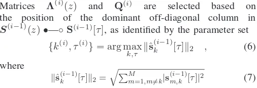
matrices Rˆ₁₂₍_z₎ _∈ C(M′−P)×P _and Rˆ₂₁₍_z₎ _∈ CP×(M′−P)_, whereRˆ₁₂₍_z_{) =}R˜ˆ₂₁₍_z₎_{are approximately zero. The} dimen-sions of the smaller matrix produced during division, P, is forced to satisfy P≤Mˆ.

The SMS algorithm is initialised and operates in a similar manner to the SMD algorithm in Sec. II-A, but with a few key differences. Instead of iteratively shifting single row-column pairs in an effort to diagonalise a parahermitian matrixS(i)₍_z_), SMS iteratively minimises the energy in select regions of S(i)₍_z₎_{in an attempt to segment the matrix. Fig. 2 illustrates} the segmentation process forM′_{= 5} _and_P_{= 2.}

To achieve this segmentation, the delay matrix (3) from SMD is replaced with paraunitary delay matrix

Λ(i)(z) = diag{1 . . . 1

| {z }

M′₋_P

z−τ(i) . . . z−τ(i)

| {z }

P

} (13)

b) a)

0

c) ^

]

^ 22]

^ 2]

^ ₂]

_R₀

0

_R

0

_R

[image:3.612.314.567.53.134.2]

_R

Fig. 2. (a) Original matrixRˆ_[_τ_]_∈C5×5

, (b) regions (red) to be iteratively driven to zero in SMS forP = 2, and (c) segmented result.NRˆ andNRˆ′

are the maximum lags for the original and segmented matrices, respectively.

Input:Rˆ₍_z_),_I_D_,_P_,_µ_,_δ

Output:Rˆ₁₁₍_z_),Rˆ₂₂₍_z_),T₍_z₎

Find eigenvectorsQ(0) that diagonaliseR[0]ˆ ∈CM′_×_M′

S(0)₍_z_{) =}Q(0)Rˆ₍_z_)Q(0)H_,H(0)₍_z_{) =}Q(0),i= 0, stop = 0

do

i=i+ 1

Findτ(i) _{from (14); generate}_Λ(i)

(z)from (13) S(i)′₍_z_{) =}_Λ(i)₍_z₎S(i−1)₍_z₎_Λ˜(i)₍_z₎

Find eigenvectorsQ(i) _{that diagonalise}_S(i)′_[0] S(i)₍_z_{) =}Q(i)_S(i)′₍_z_)Q(i)H

H(i)₍_z_{) =}_Q(i)_H(i)′₍_z_{) =}_Q(i)_Λ(i)₍_z₎_H(i−1)₍_z₎

TruncateH(i)₍_z₎_{according to (11)} TruncateS(i)₍_z₎_{according to (12)}

ifi > ID or (16) satisfiedthen

stop = 1;

end whilestop = 0 T₍_z_{) =}H(i)₍_z₎

ˆ

R₁₁₍_z₎_{is top-left}₍_M′

−P)×(M′

−P)block ofS(i)₍_z₎ ˆ

R₂₂₍_z₎_{is bottom-right}P×P block ofS(i)₍_z₎

Algorithm 2:SMS algorithm

at the ith iteration of SMS, where

τ(i)= arg max

τ kS (i−1)

21 [τ]kF (14)

and

kS(21i−1)[τ]kF= q

PM′

m=M′₋P+1

PM′−P

k=1 |S (i−1)

m,k [τ]|2 . (15)

Where S(_m,ki−1)[τ] represents the element in the mth row and

kth column of the coefficient matrix S(i−1)_[_τ_] _{at lag} _τ_.

Equations (4) and (5) are similarly implemented in SMS, where unitary matrix Q(i) _{again diagonalises}_S(i)′_[0].

AfterIDiterations, or when matrixS(21I)(z)contains energy

belowδP_τkS(I)_[_τ_]_k2

F at some iterationI; i.e.,

P

τkS (I)

21[τ]kF< δ

P

τkS( I)_[_τ_]_k2

F , (16)

the SMS algorithm returns matrices Rˆ₁₁₍_z_), Rˆ₂₂₍_z_{), and} T₍_z_{). The latter is constructed from the concatenation of the} elementary paraunitary matrices as in (10). A parameterµ is used to truncate the paraunitary and parahermitian matrices at each iteration as described in (11), (12).

The above steps of SMS are summarised in Algorithm 2.

C. Independent Conquering of Divided Polynomial Matrices

At this stage of DC-SMD, R₍_z₎ _∈ CM×M _{has been}

(4)

which are stored as blocks on the diagonal of R′₍_z_{). Each} matrix can now be diagonalised individually through the use of a PEVD algorithm; here, the SMD algorithm is chosen. Each instance of SMD is provided with a parameter IC — which

defines the maximum possible number of algorithm iterations — a stopping threshold ǫ, and a truncation parameter µ. Upon completion, the SMD algorithm returns matricesHˆ₍_z₎ and Dˆ₍_z_{), which contain the polynomial eigenvectors and} eigenvalues for input matrix A₍_z_{), respectively. At iteration}

γ of this stage, A₍_z₎ _{contains the} _γ_{th block of} R′₍_z₎ _from the bottom-right.

D. Algorithm Complexity

The instantaneous complexity of DC-SMD varies as the algorithm progresses, due to the changing spatial dimensions of the matrices being processed. The main cost of the SMS and SMD algorithms internal to DC-SMD is a matrix mul-tiplication step; therefore, the calculation of the cumulative complexities of DC-SMD is similar to Sec. II-B.

In DC-SMD, one instance of the SMS algo-rithm has a maximum cumulative complexity of

M3

α

PID

i=0(2L{S

(i)′_}₊_L_{_H(i)′_}_{), and SMD has a similar}

maximum of M3 γ

PIC

i=0(2L{S

(i)′_}₊_L_{_H(i)′_}_{), where} _M

α

and Mγ are the dimensions of the matrices input to each

algorithm, respectively. FunctionL{·}computes the length of the parahermitian and paraunitary matrix in each algorithm at iterationi. The total cumulative complexity of DC-SMD can be approximated by summing the cumulative complexities of each instance of the SMS and SMD algorithms.

From the description of DC-SMD in Algorithm 1, it can be seen that an M ×M matrix is only ever processed in the first recursion of the division step; at all other points in the algorithm, the processed matrices are of lower spatial dimension. Given that the complexity is proportional to the cube of the spatial dimension, significantly lower complexity will be observed beyond the first recursion of DC-SMD.

IV. RESULTS

To benchmark the proposed approach, this section first defines the performance metrics for evaluating the SMD and DC-SMD algorithms before setting out a simulation scenario, over which an ensemble of simulations will be performed.

A. Performance Metrics

Since SMD and DC-SMD iteratively minimise off-diagonal energy, a suitable metric Enorm(i) , defined in [9], is used; this

metric divides the off-diagonal energy in the parahermitian matrix at the ith iteration by the total energy. Computation of Enorm(i) generates squared covariance terms; therefore a

logarithmic notation of5 log10E (i)

norm is employed.

When truncation is employed, the eigenvectors and eigen-values output from SMD are only able to approximately reconstruct the input matrix. DC-SMD experiences similar error from truncation, and also introduces further error in its divide step, due to imperfect segmentation in SMS. A metric capable of measuring the difference between the original and reconstructed matrices is the mean squared error:

MSE = 1

M2_L_{_ER} P

τkER[τ]k2F, (17)

where ER[τ] = R[¯ τ]−R[τ] ∀ τ, R¯(z) = F˜(z)D(z)F(z),

andF₍_z₎_andD₍_z₎_{are obtained from SMD or DC-SMD.} The contents of Sec. II-B and Sec. III-D allow approximate measurements of cumulative complexity to be made at each iteration of both algorithms.

The output paraunitary matrix F₍_z₎ _{can be used in} sig-nal processing applications. A useful metric for gauging the implementation cost of this matrix is its length.

B. Simulation Scenario

The simulations below have been performed over an en-semble of 103 _{instantiations of} _R₍_z₎ _∈ _CM×M_, _M _∈ {20; 40}, based on the randomised source model in [9]. This source model generates R₍_z_{) =} U˜₍_z₎W₍_z₎U₍_z_{), whereby} the diagonal W₍_z₎ _∈ CM×M _{contains the power spectral}

densities (PSDs) of 10 independent sources. These sources are spectrally shaped by innovation filters such thatW₍_z₎_{has an} order of 120, and limits the dynamic range of the PSDs to about 30dB. Random paraunitary matricesU₍_z₎_∈CM×M _of order 60 perform a convolutive mixing of these sources, such thatR₍_z₎_{has an order of 240.}

During iterations, a truncation parameter ofµ= 10−6 _and

stopping thresholds ofǫ= 10−6_and_δ_{= 10}−3_{were used. The}

standard SMD implementation was run overI= 800iterations forM = 20, and I = 400iterations for M = 40. DC-SMD was executed with input parameters ID = 100, IC = 200,

P = 8, andMˆ = 8. At every iteration step of both algorithms, the diagonalisation and cumulative complexity metrics defined in Sec. IV-A were recorded together with the elapsed execution time. The MSE metric defined in (17) and the length ofF₍_z₎ were recorded upon each algorithm’s completion.

C. Diagonalisation

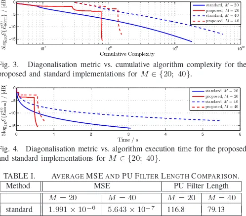
The ensemble-averaged diagonalisation was calculated for both the standard and proposed implementations. The diago-nalisation performance versus time and cumulative complexity for both methods are shown in Figs. 3 and 4, respectively. The curves of Fig. 3 demonstrate that for M ∈ {20; 40}, the proposed implementation operates with a lower cumulative complexity than the standard SMD realisation, and is able to achieve a similar degree of diagonalisation. In addition, Fig. 4 shows that the lower complexity associated with DC-SMD translates to a faster diagonalisation than observed for SMD. Using a matrix with a larger spatial dimension of M = 40 demonstrates a larger increase in diagonalisation performance with respect to execution time. In both plots, E{·} is the expectation operator.

The ’stepped’ characteristics of the curves for DC-SMD are a result of the algorithm’s recursive two-stage implementation. The divide step of the algorithm exhibits low diagonalisation for a large increase in cumulative complexity and execution time. In the conquer step, high diagonalisation is seen for a small increase in cumulative complexity and execution time.

D. Reconstruction Error

(5)

107

108

109

1010

−15 −10 −5 0

Cumulative Complexity

5l

og

1

0

E

{

E

(

i

)

n

o

rm

}

/

[d

B

]

[image:5.612.47.296.58.277.2]

standard,M= 20 proposed,M= 20 standard,M= 40 proposed,M= 40

Fig. 3. Diagonalisation metric vs. cumulative algorithm complexity for the proposed and standard implementations forM∈ {20; 40}.

0 1 2 3 4 5 6 −15

−10 −5 0

Time / s

5l

og

1

0

E

{

E

(

i

)

n

o

rm

}

/

[d

B

]

standard,M= 20 proposed,M= 20 standard,M= 40 proposed,M= 40

Fig. 4. Diagonalisation metric vs. algorithm execution time for the proposed and standard implementations forM∈ {20; 40}.

TABLE I. AVERAGEMSEANDPU FILTERLENGTHCOMPARISON. Method MSE PU Filter Length

M= 20 M= 40 M= 20 M= 40

standard 1.991×10−6

5.643×10−7

116.8 79.13 proposed 7.991×10−6

3.477×10−6

154.3 121.8

that the increased diagonalisation speed and lower cumula-tive complexity of DC-SMD comes with the cost of higher reconstruction error. To reduce this error, parameterδ can be decreased; however, this will reduce the speed and increase the complexity of the algorithm, as more effort will be contributed to the divide step. Note that the relative difference in average MSE is larger for the case whereM = 40, which suggests that the algorithm’s much improved diagonalisation performance forM = 40is not without cost.

E. Paraunitary Filter Length

The ensemble-averaged paraunitary (PU) filter lengths were calculated for both algorithms. Tab. I shows the results for

M ∈ {20; 40}. It can be seen from this table that the average paraunitary filter length is larger for DC-SMD than SMD; this is disadvantageous for application purposes. The relative difference in average paraunitary filter length is larger for the case whereM = 40, which validates the previous observation that the algorithm’s increased diagonalisation performance for

M = 40brings more substantial disadvantages.

V. CONCLUSION

We have proposed an alternative technique to compute the polynomial EVD of a parahermitian matrix; this algorithm — named DC-SMD — makes use of a divide-and-conquer approach to the PEVD, and has been shown to operate with lower computational complexity than the traditional SMD algorithm. Simulation results have demonstrated that this com-plexity reduction, and the associated execution time decrease, come with the disadvantage of increasing the mean squared reconstruction error and the paraunitary filter order.

When designing PEVD implementations for real applica-tions, the potential for the proposed techniques to increase diagonalisation performance while reducing complexity re-quirements offers benefits. A further advantage of the DC-SMD algorithm is its ability to produce multiple independent parahermitian matrices, which may be processed in parallel. Simulation results demonstrate that DC-SMD outperforms

SMD more significantly for larger values ofM; therefore, DC-SMD is suitable for broadband multichannel applications with a large number of sensors.

ACKNOWLEDGEMENT

Fraser Coutts is the recipient of a Caledonian Scholarship; we would like to thank the Carnegie Trust for their support.

This work was supported in parts by the Engineering and Physical Sciences Research Council (EPSRC) Grant number EP/K014307/1 and the MOD University Defence Research Collaboration in Signal Processing.

REFERENCES

[1] C. H. Ta and S. Weiss. A design of precoding and equalisation for broadband MIMO systems. InAsilomar SSC, pp. 1616–1620, Pacific Grove, CA, USA, Nov. 2007.

[2] P. P. Vaidyanathan. Multirate Systems and Filter Banks. Prentice Hall, Englewood Cliffs, 1993.

[3] A. Alzin, F. Coutts, J. Corr, S. Weiss, I. K. Proudler, and J. A. Chambers. Adaptive broadband beamforming with arbitrary array geometry. In

IET/EURASIP ISP, London, UK, Dec. 2015.

[4] S. Weiss, S. Bendoukha, A. Alzin, F. Coutts, I. Proudler, and J. Cham-bers. MVDR broadband beamforming using polynomial matrix tech-niques. InEUSIPCO, pp. 839–843, Nice, France, Sep. 2015. [5] I. Gohberg, P. Lancaster, and L. Rodman. Matrix Polynomials.

Aca-demic Press, New York, 1982.

[6] J. G. McWhirter, P. D. Baxter, T. Cooper, S. Redif, and J. Foster. An EVD Algorithm for Para-Hermitian Polynomial Matrices. IEEE TSP, 55(5):2158–2169, May 2007.

[7] S. Icart, P. Comon. Some properties of Laurent polynomial matrices. InIMA Int. Conf. Math. Signal Proc., Birmingham, UK, Dec. 2012. [8] P. Vaidyanathan. Theory of optimal orthonormal subband coders.IEEE

TSP, 46(6):1528–1543, June 1998.

[9] S. Redif, S. Weiss, and J. McWhirter. Sequential matrix diagonalization algorithms for polynomial EVD of parahermitian matrices.IEEE TSP, 63(1):81–89, Jan. 2015.

[10] J. Corr, K. Thompson, S. Weiss, J. McWhirter, S. Redif, and I. Proudler. Multiple shift maximum element sequential matrix diagonalisation for parahermitian matrices. InIEEE Workshop on Statistical Signal Processing, pp. 312–315, Gold Coast, Australia, June 2014.

[11] Z. Wang, J. G. McWhirter, J. Corr, and S. Weiss. Multiple shift second order sequential best rotation algorithm for polynomial matrix EVD. In

EUSIPCO, pp. 844–848, Nice, France, Sep. 2015.

[12] J. Corr, K. Thompson, S. Weiss, J. G. McWhirter, and I. K. Proudler. Causality-Constrained multiple shift sequential matrix diagonalisation for parahermitian matrices. In EUSIPCO, pp. 1277–1281, Lisbon, Portugal, Sep. 2014.

[13] J. Corr, K. Thompson, S. Weiss, I. Proudler, and J. McWhirter. Row-shift corrected truncation of paraunitary matrices for PEVD algorithms. InEUSIPCO, pp. 849–853, Nice, France, Sep. 2015.

[14] J. Foster, J. G. McWhirter, and J. Chambers. Limiting the or-der of polynomial matrices within the SBR2 algorithm. In IMA Int. Conf. Math. Signal Proc., Cirencester, UK, Dec. 2006.

[15] C. H. Ta and S. Weiss. Shortening the order of paraunitary matrices in SBR2 algorithm. InICICSP, pp. 1–5, Singapore, Dec. 2007. [16] F. Coutts, J. Corr, J. Thompson, S. Weiss, J. Proudler, and J. McWhirter.

Memory and Complexity Reduction in Parahermitian Matrix Manipu-lations of PEVD Algorithms. InEUSIPCO, pp. 1633-1637, Budapest, Hungary, August 2016.

[17] F. Coutts, J. Corr, J. Thompson, S. Weiss, I. Proudler, and J. McWhirter. Complexity and Search Space Reduction in Cyclic-by-Row PEVD Algorithms. InAsilomar SSC, Pacific Grove, CA, Nov. 2016. [18] J. J. M. Cuppen. A divide and conquer method for the symmetric

tridiagonal eigenproblem.Num. Mathematik, 36(2):177–195, June 1980. [19] J. J. Dongarra and D. C. Sorensen. A fully parallel algorithm for the symmetric eigenvalue problem.SIAM JSSC, 8(2):139–154, March 1987. [20] D. Gill and E. Tadmor. An O(N2