Structure assignment problems in linear systems: Algebraic and geometric methods

City, University of London Institutional Repository

Citation

: Karcanias, N. ORCID: 0000-0002-1889-6314, Leventides, J. and Meintanis, I.

ORCID: 0000-0002-1920-1801 (2018). Structure assignment problems in linear systems:

Algebraic and geometric methods. Annual Reviews in Control, doi:

10.1016/j.arcontrol.2018.09.004

This is the accepted version of the paper.

This version of the publication may differ from the final published

version.

Permanent repository link:

http://openaccess.city.ac.uk/id/eprint/20757/

Link to published version

: http://dx.doi.org/10.1016/j.arcontrol.2018.09.004

Copyright and reuse:

City Research Online aims to make research

outputs of City, University of London available to a wider audience.

Copyright and Moral Rights remain with the author(s) and/or copyright

holders. URLs from City Research Online may be freely distributed and

linked to.

City Research Online: http://openaccess.city.ac.uk/ [email protected]

Structure Assignment Problems in Linear Systems: Algebraic and Geometric

Methods

Nicos Karcaniasa,∗_{, John Leventides}b_{, Ioannis Meintanis}a

a_{Systems and Control Research Centre}

School of Mathematics, Computer Science and Engineering City, University of London,

Northampton Square, London EC1V 0HB, UK b_{University of Athens, Department of Economics}

Section of Mathematics and Informatics, Pezmazoglou 8, Athens, Greece

Abstract

The Determinantal Assignment Problem (DAP) is a family of synthesis methods that has emerged as the abstract formulation of pole, zero assignment of linear systems. This unifies the study of frequency assignment problems of multivariable systems under constant, dynamic centralized, or decentralized control structure. The DAP approach is relying on exterior algebra and introduces new system invariants of rational vector spaces, the Grassmann vectors and Pl¨ucker matrices. The approach can handle both generic and non-generic cases, provides solvability conditions, enables the structuring of decentralisation schemes using structural indicators and leads to a novel computational framework based on the technique of Global Linearisation. DAP introduces a new approach for the computation of exact solutions, as well as approximate solutions, when exact solutions do not exist using new results for the solution of exterior equations. The paper provides a review of the tools, concepts and results of the DAP framework and a research agenda based on open problems.

Keywords: Linear multivariable control, Structural Control Methods, Output feedback, Pole placement, Frequency assignment, Algebraic-Geometry methods

1. Introduction

Systems and Control provide a paradigm that in-troduces many open problems of mathematical nature (Rosenbrock, 1970), (Kailath, 1980), (Wonham, 1979). We distinguish two main approaches in Control The-ory, the design methodologies (based on performance criteria and structural characteristics) are mostly of iter-ative nature and the synthesis methodologies (based on the use of structural characteristics, invariants) linked to well defined mathematical problems. Of course, there exist variants of the two aiming to combine the best features of the two approaches. The Determinantal As-signment Problem (DAP) is a synthesis method and has emerged as the unified abstract problem formulation of pole, zero assignment of linear systems (Karcanias and Giannakopoulos, 1984, 1989), (Karcanias et al., 1988). DAP unifies the study of (pole, zero) frequency assign-ment problems of multivariable systems under constant,

∗_{(e-mail:[email protected])}

Quadratic Pl¨ucker Relations (QPR) (Hodge and Pedoe, 1952). There are many approaches dealing with specific frequency assignment problems (pole-zero), but they rely on specific system representations and they can-not be easily extended to deal with the whole family of constant, dynamic, decentralised problems. The affine geometry approach deals with generic cases only and it does not provide computations for exact, as well as, approximate problems. The DAP approach has the ad-vantage of introducing new system invariants of rational vector spaces in terms Grassmann vectors and Pl¨ucker matrices (Karcanias and Giannakopoulos, 1984) pro-viding a matrix characterisation of decomposability in terms of the Grassmann matrices (Karcanias and Gi-annakopoulos, 1988), (Karcanias and Leventides, 2015) and developing a novel computational framework based on the technique of Global Linearisation (GL) (Leven-tides and Karcanias, 1995). GL is based on the notion of degenerate feedback (Brockett and Byrnes, 1981) and apart from establishing solvability conditions (Leven-tides and Karcanias, 1995), also provides a linearisa-tion of the inherently nonlinear equalinearisa-tions and leads to the computation of solutions (when such solutions ex-ist). Within the DAP framework a number of solvability conditions have been established (Leventides and Kar-canias, 1995, 1992, 1993; Karcanias and Leventides, 1996) for the exact and generic frequency assignment problem. The GL methodology has in general high sen-sitivity leading to high gains in the compensation. Tech-niques such as, homotopy continuation and Newton-type schemes (Leventides et al., 2014a,b) have been used in order to be able to achieve solutions with much better sensitivity properties.

The DAP framework has been used for the study of constant and dynamic pole assignment, where low complexity solutions have been established (Leventides and Karcanias, 1998b), as well as for problems of zero assignment by squaring down (Karcanias and Gian-nakopoulos, 1989), (Leventides and Karcanias, 2009). Degenerate feedback gains (Karcanias et al., 2016b) are defined for both constant and dynamic assignment prob-lems. Parametrising the family of degenerate feedbacks gives extra degrees of freedom in computing appropri-ate controllers that linearise asymptotically DAP and enabling the selection of solutions with reduced sen-sitivity This parametrisation methodology plays a key role in selecting feasible structures for decentralized control problems. The selection of a decentralisation scheme has been handled mostly using conditions de-rived from the nature and spatial arrangement of sub-process units (Siljak, 1991). DAP can provide an al-gebraic framework for selection of the desirable

decen-tralisation (Karcanias et al., 2016c) aiming at develop-ing schemes that allow the satisfaction of generic solv-ability conditions and shaping the parametric invariants linked to solvability of decentralised control problems. DAP framework provides simple tests for avoiding fixed modes by exploiting the relationship of algebraic invari-ants (Pl¨ucker matrices) to decentralised Markov param-eters (Leventides and Karcanias, 1998a). The overall philosophy is to devise methods for design that facil-itate the solvability of decentralised control problems. Amongst the problems considered are: (i) Define the de-sirable cardinality of input, output structures to permit satisfaction of generic solvability conditions, (ii) Design the structure of input, output maps (matrices B, C) to eliminate the fixed modes and guarantee full rank prop-erties to the decentralised Pl¨ucker matrices (Leventides and Karcanias, 2006).

A significant advantage of the DAP framework is that it introduces a new approach for the computation of ex-act and approximate solutions of DAP. This is based on an alternative, linear algebra type, criterion for decom-posability of multivectors to that defined by the QPRs, in terms of the rank properties of structured matrices, re-ferred to as Grassmann matrices (Karcanias and Gian-nakopoulos, 1988), (Karcanias and Leventides, 2015). The development of the new computational framework requires the study of the properties of Grassmann ma-trices, which are further developed by using the Hodge duality (Hodge and Pedoe, 1952) leading to the defi-nition of the Hodge-Grassmann matrix (Karcanias and Leventides, 2015). Computing solutions (exact, or ap-proximate) to DAP requires the investigation of dis-tance problems, such as: (i) disdis-tance of a point from the Grassmann variety; (ii) distance of a linear variety from the Grassmann variety; (iii) parametrisation of families of linear varieties with a given distance from the Grass-mann variety; (iv) relating the latter distance problems with properties of the stability domain. The distance problems extend the exact intersection problem between the Grassmann and the linear space varieties and are related to classical problems, such as spectral analysis of tensors (Lathauwer et al., 2000), homotopy and con-strained optimization methods (Absil et al., 2008), the-ory of algebraic invariants etc.

This paper provides a review of the concepts, methodology and results of the DAP framework, as well as relevant results that complement those of the current approach. The review is then completed by providing a number of challenges for the DAP approach which form a research agenda for future activities.

whereas Section 3 presents the abstract DAP framework which is reduced to the study of polynomial combinants and the problem of decomposability of multivectors. The solvability is equivalent to finding real intersections between a linear variety and the Grassmann variety of a projective space. DAP introduces new invariants of ra-tional vector spaces defined by the Grassmann vectors and the Pl¨ucker matrices. Section 4, deals with the de-composability of multivectors where first the Quadratic Pl¨ucker Relations and then a new test for decomposabil-ity provided by the rank properties of the Grassmann matrix is presented. Section 5, examines the solvability of DAP under the genericity assumption. We focus on determining real solutions and a number of results are reviewed derived from the DAP framework and other re-lated approaches. Section 6, deals with the GL method-ology by examining the properties of the pole placement map, the notion of degenerate compensators with their parametrisation and the sensitivity of such solutions. Section 7, extends the GL methodology to decentral-ized control problems. The parametrisation of the fam-ily of decentralized degenerate schemes is linked to the selection of appropriate asymptotic linearising decen-tralized schemes capable of assigning the closed loop poles. Section 8, deals with the computation of exact and approximate solutions of DAP, in terms of the prop-erties of structured matrices, the Grassmann and Hodge-Grassmann matrices. Finally, Section 8 provides a list of open questions related to the DAP framework which form a future research agenda.

Notation: Throughout the paper the following nota-tion is adopted: If Fis a field, or ring then Fm×n

de-notes the set ofm×nmatrices overF. R[s] is the ring

of polynomials and_R(s) is the field of rational func-tions over_R respectively. If H is a map, then R(H), N_r(H),N_l(H) denote the range, right, left null-spaces respectively. Qk,n denotes the set of lexicographically

ordered, strictly increasing sequences ofkintegers from the set ¯n = {1,2, . . . ,n}. If V is a vector space and {v_i

1, . . . ,vik}are vectors ofVthenvi1∧. . .∧vik =vω∧,

ω=(i1, . . . ,ik) denotes their exterior product and∧rV

ther−th exterior power ofV (Marcus, 1973). IfH ∈

Fm×n andr 6 min{m,n}thenCr(H) denotes ther−th

compound matrix of H (Marcus and Minc, 1964). In most of the following, we assume thatF=R, orC.

2. The Determinantal Assignment Problems in Control Theory

2.1. Introduction

The DAP methodology (Karcanias and Giannakopou-los, 1984) has been formulated as a unifying approach

for all pole, zero frequency assignment problems with constant and dynamic compensators. This framework may be also applied to the case of decentralised control problems.

2.2. Control Problems leading to the DAP formulation

Consider the linear system,S(A,B,C), described by:

˙

x=Ax+Bu, A∈_Rn×n,B∈_Rn×p (1)

y=C x, C∈_Rm×n

where (A,B) is controllable, (A,C) is observable, or equivalently the transfer function matrix G(s) =

C(sI−A)−1Bhasrank_R(s){G(s)}=min (m,p). In terms of Left, Right Coprime Matrix Fraction Descriptions (LCMFD, RCMFD) (Kailath, 1980),G(s) may be rep-resented as

G(s)=Dl(s)−1·Nl(s)=Nr(s)·Dr(s)−1 (2) where, Nl(s),Nr(s) ∈ _R[s]m×p _{and Dl(s) ∈}

R[s]m×m,

Dr(s) ∈ _R[s]p×p_{. The following frequency assignment}

problems are defined:

(i) Pole assignment by state feedback: ConsiderL ∈

Rn×p, whereLis a state feedback applied on system (1).

The state feedback design involves finding L ∈ _Rn×p assigning the closed loop characteristic polynomial:

pL(s)=det{sI−A−BL}=det{B(s)·_L˜} (3)

where,B(s)=[sI−A,−B] and ˜L=_In,_Ltt_.

(ii) Design of an n−state observer: The design prob-lem of ann−state observer for system (1) involves find-ing an output injection,T ∈_Rn×m_{, such that the}

charac-teristic polynomial of the observer is:

pT(s)=det{sI−A−T C}=det{T˜·C(s)} (4)

where, ˜T =[In,T] andC(s)=sI−At,−Ct t

.

(iii) Pole assignment by constant output feedback: For the system described by (2), the constant output feedback design problem requires finding a matrixK ∈

Rm×pthat assigns the closed loop pole polynomial:

pK(s)=det{Dl(s)+Nl(s)·K}=det{Dr(s)+K·Nr(s)}

or, equivalently

pK(s)=det{Tl(s)·Kl˜}=det{Kr˜ ·Tr(s)} (5)

by defining the composite matricesTl(s)∈_R[s]m×(m+p)_,

Tr(s)∈_R[s](m+p)×p_{, ˜Kl∈}

R(m+p)×m, ˜Kr∈Rp×(m+p)

Tl(s)=[Dl(s),Nl(s)] Kl˜ =hIm,Kti

Tr(s)=

"

Dr(s)

Nr(s)

#

˜

(iv) Zero assignment by squaring down: For a sys-tem with m > p we can expect to have independent control over at most p−linear combinations ofm out-puts. Ifc∈ _Rp _{is the vector of the variables which are}

to be controlled, then, c = Hy, whereH ∈ _Rp×m _{is a}

squaring down post-compensator, andG0(s)=H·G(s) is the squared down transfer function matrix (Karca-nias and Giannakopoulos, 1989). A right MFD for

G0(s) is defined by G0(s) = H · Nr(s)Dr(s)−1 _where

G(s) = Nr(s)Dr(s)−1_{. Finding H such that G}0 (s) has assigned zeros is defined as the zero assignment by squaring down problem. The zero polynomial of

S(A,B,HC,HD) is given by:

zk(s)=det{H·Nr(s)} (6)

Figure 1: Feedback configuration.

(v) Dynamic Compensation Problems: Consider the standard feedback configuration (Kucera, 1979) shown in Fig.1. IfG(s)∈_R(s)mpr×p,C(s)∈R(s)ppr×m, and assume

coprime MFDs as in (2) and

C(s)=Al(s)−1·Bl(s)=Br(s)·Ar(s)−1 (7) the closed loop characteristic polynomial is

f(s)=det

(

[D`(s), N`(s)]

"

Ar(s)

Br(s)

#)

(8)

f(s)=det

(

[Al(s), Bl(s)]

"

Dr(s)

Nr(s)

#)

(9)

If p ≥ m, the C(s) may be interpreted as pre-compensator (8); whereas, if p ≤ m, then C(s) may be interpreted as feedback compensator (9). The above general dynamic formulation covers a number of impor-tant families ofC(s)−compensators as:

Constant Controllers: If p ≤ m,Al = Ip, Bl = K ∈

Rp×m, then (9) expresses the constant output feedback

case; whereas ifp ≥m,Ar = Im,Br = K ∈ _Rp×m

ex-presses the constant pre-compensation.

Proportional plus Integral Controllers:

C(s)=K0+ 1

sK1=

h

sIpi−1[sK0+K1] (10)

where,K0,K1 ∈Rp×mand the left MFD forC(s) is

co-prime, if and only if,rank(K1)=p. Then, f(s) is:

f(s)=det

(

[sIp,sK0+K1]

"

Dr(s)

Nr(s)

#) (11) =det         

[Ip,K0,K1]

         

sDr(s)

sNr(s)

Nr(s)

                  

Proportional plus Derivative Controllers:

C(s)=sK0+K1=

h

Ipi−1[sK0+K1] (12) where,K0,K1 ∈Rp×mand the left MFD forC(s) is

co-prime for finite sand also fors =∞ifrank(K0)= p. Then, f(s) is:

f(s)=det

(

[Ip,sK0+K1]

"

Dr(s) Nr(s)

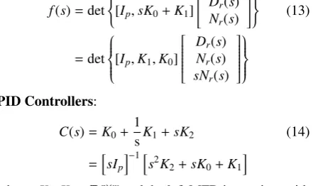
#) (13) =det         

[Ip,K1,K0]

         

Dr(s) Nr(s) sNr(s)

                  

PID Controllers:

C(s)=K0+ 1

sK1+sK2 (14)

=h

sIpi−1hs2K2+sK0+K1

i

where,K0,K2∈Rp×mand the left MFD is coprime with

the only exception possibly at s=0, s=∞ (coprime-ness at s = 0 is guaranteed by rank(K1) = p and at

s=∞byrank(K2)=p). Then,f(s) is expressed as:

f(s)=det

(

[sIp,s2K2+sK0+K1]

"

Dr(s) Nr(s)

#) =det               

[Ip,K0,K1,K2]

             

sDr(s) sNr(s) Nr(s) s2_Nr(s)

                             (15)

The problems introduced here belong to the same fam-ily, DAP, involving solving the following equation with respect to polynomial matrixH(s):

det{H(s)·M(s)}=f(s) (16)

3. The Abstract DAP, the Projective Geometry Ap-proach and Grassmann Invariants

3.1. Introduction

The determinantal nature of DAP demonstrates that it is of a multilinear nature. Such problems may be natu-rally split into a linear and multilinear problem (decom-posability of multivectors). The final solution is thus reduced to the solvability of a set of linear equations together with quadratics (characterising the multilinear problem of decomposability).

3.2. The Decomposition of DAP

The family of DAP problems requires solving

det{H(s)·M(s)}= f(s) (17) with respect to polynomial matrixH(s), where f(s) ∈

R[s] withdeg(f(s))=nandM(s) is a polynomial

ma-trix related to the system and the problem under study. The difficulty in solving DAP is due to the multilinear nature of the problem. Note that all dynamic problems may be reduced to equivalent constant DAP by shifting all dynamics fromH(s) toM(s) and defining an equiv-alent matrixM(s)∗.

Remark 1. The reduction of dynamic DAP problems to equivalent constant is evident from the formulation of general dynamic DAP problems, as indicated for in-stance, by conditions (11), (13), (15) for the PI, PD and PID design problems respectively. The shifting of dy-namics implies development of appropriate augmented design matricesM(s) (M(s)∗_).

LetM(s) ∈ _R[s]p×r,r ≤ p, such thatrank{M(s)} =r

and letHbe a family of full rankr×pconstant matrices

Hhaving a certain structure defined by the nature of the system and the type of compensation. The degree of

f(s) depends upon the degree ofM(s) and the structure ofH∈ H. Hence, (17) is equivalent to

fM(s,H)=det{H·M(s)}= f(s) (18)

If h_it, m_i(s),i ∈ r¯, denote the rows of H ∈ _Rr×p_,

columns ofM(s)∈_R[s]p×r_{respectively, then} Cr(H)=h₁t∧. . .∧h_rt=ht∧ ∈_R1×σ

Cr(M(s))=m₁(s)∧...∧m_r(s)=m∧ ∈_Rσ[s] whereσ=p_r. By Binet-Cauchy theorem (Marcus and Minc, 1964) we have that (Karcanias and Giannakopou-los, 1984):

fM(s,H)=Cr(H)·Cr(M(s))=

D

h∧,m(s)∧E

= X

ω∈Qr,p

hω·mω(s) (19)

where,h·,·idenotes the inner product,ω=(i1, . . . ,ir)∈

Qr,p, andhω,mω(s) are the coordinates ofh∧,m(s)∧

re-spectively. Note thathω is ther×rminor ofHwhich

corresponds to theω-set of columns ofH and thushω

is a multilinear alternating function of the hi j entries.

The multilinear nature of DAP suggests that the natu-ral framework for its study is of exterior algebra. The essence of exterior algebra is that it reduces the study of multilinear skew-symmetric functions to the simpler study of linear functions. An example on how to com-pute the exterior product for a set of vectors is given below.

Example 1. For a set of 2 vectors in R4 with

coordi-nates

a11 a12 a13 a14

a21 a22 a23 a24

!

the exterior product can be computed by taking all the 2×2 minors lexicographically ordered:

C2(A)=(|A(1,2)|,|A(1,3)|,|A(1,4)|, |A(2,3)|,|A(2,4)|,|A(3,4)|)

where,|A(i,j)|denote the 2×2 minors of matrixA con-sists of thei,j-th columns lexicographically ordered.

The study of the zero structure of fM(s,H) may thus be

reduced to a linear subproblem and a standard multilin-ear algebra subproblem:

Linear sub-problem of DAP: Set m(s)∧ = p(s) ∈

Rσ[s]. Determine whether there exists ak∈Rσ,k,0,

such that for f(s)∈_R[s]

fM

s,k=kt·p(s)=X

i∈σ

ki·pi(s)= f(s) (20)

Multilinear sub-problem of DAP: Assume that K is the family of solution vectors k of (20). Determine whether there existsHt=hh₁, . . . ,h_ri∈_Rp×r_{such that}

h₁∧ · · · ∧h_r=h∧=k, k∈ K (21)

Vinto an appropriate projective spacePσ−1_{,σ = p}

r

. This map is referred to as the Pl¨ucker Embedding (Mar-cus, 1973) of the GrassmanianHinto a projective space Pσ−1_{. Thus, we are searching for common solutions of} some set of linear equations and another set of second order polynomial equations, i.e. the set of Quadratic Pl¨ucker Relations (QPRs) characterising the Grassman variety of Pσ−1 _{(Hodge and Pedoe, 1952), (Marcus,} 1973). This also allows us to compactifyHinto ¯Hand then use algebraic geometric, or topological intersec-tion theory methods to determine existence of soluintersec-tions for the above sets of equations. The current framework allows the use of algebraic geometry and topological methods (Brockett and Byrnes, 1981), (Byrnes, 1989), (Leventides and Karcanias, 1992) for the study of solv-ability conditions but also computations.

3.3. The Grassmann and Pl¨ucker Invariants of a Rational Vector Space

The DAP framework uses the natural embedding of a Grassmannian into a projective space and this in turn de-fines new sets of invariants characterising the solvabil-ity of the different DAP problems. We may summarise the main results next (Karcanias and Giannakopoulos, 1984):

Let T(s) = ht₁(s), . . . ,t_r(s)i ∈ _Rp×r_{(s), r ≤ p,} rank{T(s)}=randXt =rowspanR(s){T(s)}. IfT(s)=

M(s)D(s)−1 is a RCMFD ofT(s), thenM(s) is a poly-nomial basis forXt. IfQ(s) is a greatest right divisor

ofM(s) thenT(s)= M˜(s)Q(s)D(s)−1, where ˜M(s) is a least degree polynomial basis ofX_t(Rosenbrock, 1970). A Grassmann Representative (GR) forX_tis defined by

t(s)∧=t₁(s)∧. . .∧t_r(s)

=m˜₁(s)∧. . .∧m˜_r(s)·zt(s)/pt(s)

where,zt(s)=det{Q(s)},pt(s)=det{D(s)}are the zero, pole polynomials ofT(s) and ˜m(s)∧ = m˜₁(s)∧. . .∧

˜

m_r(s)∈_Rσ[s], is also a GR ofXt. Since, ˜M(s) is a least

degree polynomial basis forX_t, the polynomial entries of ˜m(s)∧are coprime and it will be referred to as a re-duced polynomialGR ofX_t. Ifδ = deg{m˜(s)∧}, then

δis the Forney dynamical order (Forney, 1975) ofX_t. ˜

m(s)∧may always be expressed as

˜

m(s)∧=p(s)=p

0+sp1+· · ·+s

δ_p

δ=Pδ·eδ(s) (22)

where, Pδ ∈ Rσ×(δ+1) is a basis matrix for ˜m(s)∧and

e_δ(s) = h1,s, . . . ,sδit. By choosing an ˜m(s)∧ with kPδk = 1, a canonical R[s]−GR ofXt is defined

de-noted byg(X_t). The basis matrixPδofg(Xt) is defined

as the Pl¨ucker matrix ofXt. The following properties

hold true (Karcanias and Giannakopoulos, 1984):

Theorem 1. The R[s]−GR, g(Xt), or the associated Pl¨ucker matrix, Pδ, is a complete invariant ofXt. Remark 2. LetT(s)=ht₁(s), . . . ,t_r(s)i∈_Rp×r_{(s),r ≤}

p,rank{T(s)} = r, andzt(s), pt(s) be the monic zero,

pole polynomials of T(s) and letg(X_t) = p(s) be the

C−_R[s]−GR ofXt.t(s)∧may be uniquely decomposed

as

t(s)∧=c·p(s)·zt(s)/pt(s) (23) and the linear part of DAP is thus reduced to

fMs,k=ktp(s)zm(s)=kt·Pδ·e_δ(s)·zm(s) (24) The zeros of T(s) are fixed zeros of all combinants of

t(s)∧.

The freely assigned zeros of fMs,k are those of the

combinant fM

s,k = kt·m(s)∧, where m(s)∧ is re-duced. Ifa(s)=at

δeδ(s)=a0+a1s+· · ·+aδsδ∈R[s] is the polynomial to be assigned, thenmax(deg(a(s))=δ, whereδis the Forney dynamical order ofXt, and finding k∈_Rσ, such that fMs,k=a(s), is reduced to:

Pt_δ·k=a (25)

Remark 3. Let M(s) ∈ _Rp×r[s] be a least degree ma-trix, Pδ be the Pl¨ucker matrix of X_m and let π =

rank(Pδ). Then, necessary and sufficient condition for

M(s) to generate a DAP that is Linearly Assignable (LA) (no decomposability constraints) is thatπ=δ+1.

3.4. The Grassmann and Pl¨ucker Invariants of a system

Pl¨ucker type matrices associated with state space de-scriptions are defined (Karcanias and Leventides, 1996):

Controllability Pl ¨ucker Matrix: For the pair (A,B),

b(s)t∧denotes the exterior product of the rows ofB(s)= [sI−A,−B] andP(A,B) is the (n+1)×n+_npbasis matrix ofb(s)t_{∧.P(A,B) is theControllability Pl¨uckermatrix.}

Corollary 2. The system S(A,B)is controllable if and only if b(s)t∧is coprime, or equivalently P(A,B)has full rank.

Example 2. Consider the systemS(A,B) described by the pencil [sI−A,−B]=R(s)

         

s −1 0 0

0 s −1 0 0 0 s −1

         

=

         

r₁(s)t r₂(s)t r₃(s)t

         

The exterior product of the rows of R(s) is defined by the minors of maximal order ofR(s) lexicographically ordered, i.e.

and the Controllability Pl¨ucker matrix,P(A,B), is then

P(A,B)·e₃(s)=

             

1 0 0 0 0 −1 0 0 0 0 1 0 0 0 0 −1

              | {z }

P(A,B)

             

s3

s2

s

1

             

Clearly,P(A,B) has full rank and hence the system is

controllable.

A similar result for observability may be stated using duality principle.

Transfer Function Matrix Pl ¨ucker Matrices: For the transfer function matrix G(s) represented by the RCMFD, LCMFD we define byt_r(s)∧,t_l(s)t_∧the

ex-terior product of the columns ofTr(s), rows ofTl(s) re-spectively , whereTr(s),Tl(s) are defined by (2). By

P(Tr) we denote them+_pp×(n+1) basis matrix oft_r(s)∧, and byP(Tl) the (n+1)×m_p+pbasis matrix fort_l(s)t_∧. P(Tr),P(Tl) will be referred to asright, left fractional Pl¨ucker matrices respectively. Such matrices provide the necessary conditions for the solvability of pole as-signment problems by output feedback.

Proposition 3(Leventides and Karcanias (1995)). For a generic system with mp>n, then the Pl¨ucker matrices P(Tr), P(Tl)have full rank.

Column, Row Pl ¨ucker Matrices: For the transfer func-tionG(s), withm ≥ p, we denote byn(s)∧the exte-rior product of the columns of the numeratorNr(s), of a RCMFD and byP(N) them_l×(d+1) basis matrix of

n(s)∧. Note thatd =δ, the Forney order ofX_t, ifG(s) has no finite zeros andd=δ+k, wherekis the number of finite zeros ofG(s) otherwise. IfNr(s) is least degree,

thenPc(N) will be called thecolumn space Pl¨ucker

ma-trix of the system. Therow space Pl¨uckermatrixPr(N)

may be similarly defined whenm ≤ p. Such matrices play a key role in the study of squaring down problems (Karcanias and Giannakopoulos, 1989).

Proposition 4. For a generic system with m > p, for which p(m−p) > δ+1, whereδis the Forney order, Pc(N)has full rank.

Similar definitions and invariant may be defined for dy-namic compensation transfer function matrices.

4. Decomposability of Multivectors and the Grassmann Variety

4.1. Introduction: Decomposability of Multivectors

The solution of DAP is reduced to finding amongst the family of solutions, K, of the linear problem in (20),

at least a solutionk∈ K that also satisfies the exterior equation (21). The set ofr−dimensional subspaces of

Rp is referred to as ther−Grassmaniann and the row

space ofH,H, defines a basis for such subspaces. The mapping of eachr−dimensional subspaceHexpressed

byh₁∧. . .∧h_r=h∧r_{=k, whereh}

iare the row vectors

of H, is a vectork ∈ _Rσ, k , 0 that defines a point

in the projective space Pσ−1₍

R), σ =

_p

r

; for some

H ∈ _Rr×p_{, the points of P}σ−1 _{which satisfy (21) are} those which belong to the Grassmann varietyΩ(r,p) of Pσ−1₍

R). The coordinateskω,ω=(i1, ....,ir)∈Qr,pare

referred to as the Pl¨ucker coordinatesofk ∈ _Rσ, and the mapping ofH through∧r _{is known as thePl¨ucker} Embeddingof ther−Grassmaniann intoPσ−1₍

R). The

characterisation of theΩ(r,p) variety and the construc-tion of the subspaces H corresponding tok ∈ Ω(r,p) are considered next.

4.2. The Grassmann Variety and the Quadratic Pl¨ucker Relations

The varietyΩ(r,p) is characterised by the result (Mar-cus, 1973):

Theorem 5. Necessary and sufficient condition for an H=hh₁, . . . ,h_rit∈_Rr×p_{to exist, such that}

h∧=h₁∧. . .∧h_r=k=[. . . ,kω, . . .] (26)

is that the coordinates kωsatisfy the following quadratic

relations

r+1

X

k=1

(−1)v−1ki1,...,ir−1,j k

vj1, ...,jv−1,jv+1,jr+1=0 (27)

where,1 ≤i1 <i2 < . . . < ir−1 ≤n and1 ≤ j1 < j2 <

. . . < jr₊1≤n.

The vectorskwhich satisfy (27) are known as decom-posable and the set of quadratics defined by (27) as Quadratic Pl¨ucker Relations (QPR) (Hodge and Pedoe, 1952), (Marcus, 1973) and they define the Grassmann variety ofPσ−1(R). Interesting questions are: (i)

Defin-ing alternative conditions for decomposability; (ii) Re-constructing the matrix H for a decomposablek; (iii) Characterising the distance of a general k ∈ Pσ−1(R)

from the Grassmann varietyΩ(r,p). The reconstruction ofHfrom the decomposablekis given in Giannakopou-los et al. (1985) and in Section 4.3.

Corollary 6. Let k =[. . . ,kω, . . .]t ∈_Rσ, be a decom-posable vector and let ka1,...,ar be a non-zero coordinate

of k. If we define by

hi j=ka1,...,ai−1,j,ai+1,...,ar, i∈r¯,j∈ p¯ (28)

The procedure for constructingHfor a decomposablek

also requires writing down an independent set of QPRs which completely describesΩ(r,p).

Example 3. Assume p = 4, r = 2 and let {x12,x13,x14,x23,x24,x34} be the coordinates of a vec-tor in∧2

R4. The Grassmann varietyΩ(2,4) is defined

by the single QPR:

x12x34−x13x24+x14x23=0

4.3. The Grassmann Matrix and Decomposability of Multivectors

The Grassmann matrix ofz ∈ ∧r_(H

r) (Karcanias and

Giannakopoulos, 1988) is introduced and a number of its properties are examined. This matrix provides an alternative test for decomposability ofz, which also al-lows the computation of theHrsolution space in an easy

manner.

Proposition 7 (Marcus (1973)). Let U be a

p−dimensional vector space over F and let

0 , z ∈ ∧rU. Then, z is decomposable, if and

only if, there exists a set of linearly independent vectors

{hi,i∈r¯}inUsuch that

v_i∧z=0,∀i∈p¯ (29)

Lemma 8. Let BU ={u_i,i∈ p¯}be a basis ofU, Br_U =

{u_ω∧, ω∈Qr,p}be a basis ofUthe corresponding ba-sis of∧r_{U and let v =}Pr

t=1 ctut, z =

P

ω∈Qr,paωuω∧.

Then,

v∧z= X

γ∈Qr+1,p

bγu_γ∧ bγ=

r+1

X

k=1

(−1)k−1cγ(k)aγ(ˆk)

where, γ(k) denotes the k−th element of

γ(k) ∈ Qr+1,p and γ(ˆk) is the sequence

{γ(1), . . . , γ(k−1), γ(k+1), . . . , γ(r+1)} ∈Qr,p. Notation:Letγ=(j1,j2, . . . ,jk,jr+1)∈Qr+1,pwithr+

16p. We denote byQγ_r,r+1the subset ofQr,psequences

with elements taken from theγset of integers.Qγ_r,r+1has

r+1 elements and the sequences in it are defined from

γby deleting an index inγ. Thus, for allk∈r+1

Qγ_r,r+1=nργ[ ˆjk]=(j1, . . . ,jk−1,jk+1, . . . ,jr+1)

o

Definition 1. Let{aω, ω ∈ Qr,p}be the coordinates of z∈ ∧r_{Uwith respect to a basisB}r

U of∧

r_U,r+1

6p,

γ=(j1, . . . ,jk,jr+1)∈Qr+1,p. We define

φ:{i:i=1, . . . ,p} ×nγ, γ∈Qr₊1,p

o

→ F (30)

with,ργ[ ˆjk]=(j1, . . . ,jk−1,jk+1, . . . ,jr+1)∈Q

γ

r,r+1

φi

γ =φγ(i)=0 ,i f i,γ

φi

γ =φγ(i)=sign

jk:ργ[ ˆjk]aργ[ ˆj_k]

,i f i= jk∈γ

where,

signjk:ργ[ ˆj_k]=sign(jk,j1, . . . ,jk−1,jk+1, . . . ,jr+1).

Theorem 9(Karcanias and Giannakopoulos (1988)). If BU = {ui,i ∈ p¯}, B

r

U = {uω∧, ω ∈ Qr,p} are bases of U, ∧r_{U, v =} Pn

i=1 ciui ∈ U : v , 0, and z =

P

ω∈Qr,p

aωuω∧ ∈ ∧rU : z , 0. Then, v∧z = 0, if and

only if, n

X

i=1

φi

γci=0, for allγ∈Qr+1,p (31)

If we denote byγtthe elements of Qr+1,p (lexicograph-ically ordered), with t = 1,2, . . . ,_r+p₁ = τ, then (31) may be expressed as

                          φ1

γ1, φ

2

γ1, . . . , φ

i

γ1, . . . , φ

p

γ1

..

. ... ... ...

φ1

γt, φ 2

γt, . . . , φ

i

γt, . . . , φ

p

γt

..

. ... ... ...

φ1

γτ, φ

2

γτ, . . . , φ

i

γτ, . . . , φ

p γτ                           | {z }

Φr p(z)

                              c1 c2 .. . ci .. . cp                              

|{z}

c

=0

(32)

The matrixΦr

p(z)∈Fτ×pis a structured matrix (has

ze-ros in fixed positions), it is called theGrassmann Matrix

(GM) ofzand it is defined by the pair (r,p) and the co-ordinates{aω, ω∈Qr,p}ofz∈ ∧rU.

Theorem 10 (Karcanias and Giannakopoulos (1988)). LetU be an n−dimensional vector space overF, BU

a basis ofU, 0 , z ∈ ∧rU,Φrp(z)the GM of z)with respect to BUand letNrp(z)=Nr{Φrp(z)}. Then,

(i) dimNr

p(z)6r and equality holds, if and only if z is decomposable.

(ii) If dimNr

p(z)=r, then a representation of the solu-tion space,Hzof h₁∧. . .∧h_r =z with respect to

Uis given byNr_p(z).

Corollary 11. LetΦrp(z)be the GR of z∈ ∧rU, z,0. Then,

i) If r=1then for all p,Φ1_p(z)is always canonical; furthermore, if p_>3rankF

n

Φ1

p(z)

o

=p−1.

ii) If r=p−1, thenΦpp−1(z)∈ F1×pand it is always canonical with rankF

n

Φp−1

p (z)

o

=1.

iii) If r = p−ρ, p > 1, andρ ≥ 2, then for all z, rankF

n

Φ1

p(z)

o

≥p−ρ, where equality holds, if and only if,Φr

p(z)is canonical.

5. Real Intersections of the Grassmann Variety and Linear Space: Generic Solvability Conditions

DAP can be formulated as an intersection problem be-tween a linear variety,LR, and the Grassmann variety,

Gp(Fm+p) of a projective space, where the fieldFis

con-sidered to be eitherR(real) orC(complex).

Proposition 12. The set of (finite and infinite) real so-lutions of the constant pole assignment problem is given by

LR∩ Gp Rp+m (33)

where, LR is a linear variety of co-dimension (n) in

P(R)σ−1defined by the linear DAP sub-problem.

The real constant pole assignment problem is generi-cally solvable if and only if the intersection (33) is non-void. (Similarly is defined the generic solvability for the complex case). The real solvability of the inter-section problem (33) is challenging due to the lack of strong intersection theorems when the definition field of the problem is not algebraically closed. For instance, in the simple case of one polynomial equation with one un-known real solvability is not guaranteed. The only thing we can say is that when the degree of the polynomial is odd there exists at least one real solution. In contrast, re-garding the complex solvability case, we know that we have always as many roots as the degree of the polyno-mial to be assigned. The main results on the solvability of the output feedback pole assignment problem via the intersection theory are summarised below:

Theorem 13(Leventides and Karcanias (1992)). A suf-ficient condition for the existence of real solutions of the output feedback pole assignment problem for a generic proper system (p−inputs, m−outputs, n−states) is

h(p,m)_>n (34)

where, h(p,m)is the height of the first Whitney class(w)

(Hiller, 1980) of a real GrassmannianGp(Rp+m).

The first important result on this problem was given in Kimura (1975) and Davison and Wang (1975), where they showed that for a strictly proper system a sufficient condition for generic pole placement is that

m+p−1_>n

Using tools from algebraic geometry (Hermann and Martin, 1977), (Giannakopoulos and Karcanias, 1985) showed that a necessary and sufficient condition for ar-bitrary pole assignment by complex (constant) output feedback ism·p_>n, whereas, a special case (m·p=n

andd(m,p) = odd) was proved to be a sufficient con-dition for generic pole assignment via real output feed-back (Brockett and Byrnes, 1981).

A similar nature condition for arbitrary pole assignment of real poles using other topological invariants of the Grassmannian were given in Byrnes (1983) in terms of

LS cat(p,m)_>n (35)

where, LScatis the Ljusterning Snirelman category of the GrassmannianG_p(_Rp+m_{). In both complex and real}

cases the intersections (33) may be represented as cer-tain elements of the corresponding cohomology ring, i.e. H∗Gp(Rp+m);Z2

where the existence of inter-section is then reduced to whether these elements are nonzero. The intersection points are considered mod-2 (i.e. odd number of points correspond to one and even number of points to zero). This element is of the form

wn_{, wherewis the first Whitney class (Hiller, 1980) of}

the Grassmannian and n is the number of poles to be placed. Hence, for a generic real solution we require

wn

, 0. If we let h(p,m) the highest exponent,h, of

w∈ H∗Gp(Rp+m);Z2

so thatwh ,0, then a sufficient

condition for real solvability of DAP isn6h(p,m). It is worth noting that not all intersections (33) correspond town. It is only the intersections for which some regu-larity condition holds true. Note that, since

m+p−16h(p,m)6m·p (36)

6. The Global Linearisation Methodology

The solvability of DAP may be seen as a problem of finding real intersections between the linear variety and the Grassmann variety of an appropriate projec-tive space. An approach that applies to generic and given systems which leads to establishing of existence results and also provides a computation scheme, has been based on the notion of degenerate feedback solu-tions; this is referred to as Global Linearisation (GL) (Leventides and Karcanias, 1995). Degenerate solutions have been introduced in (Brockett and Byrnes, 1981) as the compensation solutions where the feedback con-figuration vanishes. Such solutions have the signifi-cant property that linearise asymptotically the multilin-ear nature of DAP and thus lead to the computation of solutions. The GL approach leads to numerical meth-ods to design feedback laws for DAP applications capa-ble to handle dynamic schemes, as well as structurally constrained compensation schemes (Leventides et al., 2014a,b). Furthermore, it has provided new solvability of control problems for both generic and non-generic cases.

6.1. The Pole Placement Map (Primitive Results)

Consider the pole placement problem via constant out-put feedback. The closed-loop pole polynomial is

det [I,K]·

"

D(s)

N(s)

#!

=det ([I,K]·M(s))=p(s) (37) where,M(s)∈_R[s](p+m)×pis the composite MFD of the open-loop system transfer functionG(s)=N(s)·D−1(s), [I,K] ∈ _Rp×(m+p) _{are the generalised finite feedback} compensators withK ∈_Rp×m_{andp(s) the target}

poly-nomial to be assigned.

Solvability conditions of the pole placement problem under complex and real output feedback have been es-tablished in Leventides and Karcanias (1992) based on the dimension of thePole Placement Map(PPM) and in particularly the image of the maps:

Pole Placement Map (PPM): The PPM under real (or complex) output feedback which maps every K to

p=(pn, . . . ,p1) under the relation (37) is defined by

PPM: Fp×m→Fn: PPM(K)=p (38)

where, _F is either _R (for real) or _C (for complex). The solvability of the arbitrary pole placement problem is translated into onto properties of the related PPM. For the complex case there are results based on Shard Theorem (Byrnes, 1983). In Leventides and Karcanias

(1993) the global onto properties of a polynomial map can be proved by the local onto properties of the map (linear) i.e. the differential of the mapping at a point is onto, which requires only to test the rank of a jacobian matrix (differential).

Procedure: The computational procedure involves: (i) express the PPM; (ii) calculate the differential at any point; (iii) select a specific point that the differential is easily calculated (linear map); (iv) calculate the rank of the differential of the related PPM ; (v) if the rank of the differential is full then the PPM is almost onto. It has been proved that for a generic proper system ar-bitrary pole placement is solvable with complex con-trollers when m· p > n (Byrnes, 1983), (Leventides and Karcanias, 1992). However, this procedure answers only the existence of solutions and does not lead to a construction of such solutions. Next, we summarize the main early results as far as sufficient conditions for generic pole placement.

Theorem 14. Sufficient conditions of generic systems for pole placement via complex controllers are given:

(i) m+p−1_>n; in Kimura (1975)

(ii) mp>n; in Byrnes (1983); Leventides and Karca-nias (1992)

whereas, for pole placement via real controllers the main results have been given by:

(i) LS cat(p,m)_>n; in Byrnes (1983)

(ii) h(p,m)_>n; in Leventides and Karcanias (1992)

(iii) mp = n (holds when the degree of G_p(Rp+m) is

odd); in Brockett and Byrnes (1981).

A first breakthrough regarding the sufficiency of the static generic pole assignability was established by Wang (1992) as, m· p > n. Using geometric tech-niques Rosenthal and Wang (1996, 1997) derive that,

6.2. Degenerate Solutions

Degenerate gains were first introduced by Brockett and Byrnes (1981) in their generalized form as follows:

Definition 2. A generalized gain,D=rowspan(A,K), is degenerate if and only if satisfies equation:

det ([A,K]·M(s))≡0 (39)

Degenerate gains can be constructed easily from the null-spaces of certain matrices (Wang, 1992), (Leven-tides and Karcanias, 1995). In the following we denote byM = colsp(M(s)), the_R[s]−module generated by the columns of the system composite MFDM(s).

Theorem 15. For the system represented by composite MFD, M(s)∈_R[s](m+p)×p_{, a p−dimensional space, D=} rowspan(A,K), corresponds to degenerate gain if and only if either of the following two conditions hold true:

(i) There exists an(m+p)×1polynomial vector, m(s)∈ M, such that(A,K)·m(s)=0,∀s∈_C

(ii) There exists an (m+ p)× 1 polynomial vector, m(s) ∈ M, with coefficient matrix Pm such that rank(Pm)6m.

The following example illustrates the standard proce-dure for constructing degenerate points.

Example 4. Consider a p = 2−input, m = 3−output system with n = 5 states represented by M(s) =

h

D(s)t _N(s)t it

M(s)=

                   

s3 ₀

1 s2

s2+1 s+1

s+3 s

s+1 1

                   

=h

m₁(s) m₂(s) i

To construct a degenerate point, we select a polynomial vectorm(s)∈ Mwith the lowest (column) degree, i.e.

m(s) = m₂(s) = h 0 s2 _{s+1 s 1} it

and extract its coefficient matrix, hence we express it as:

m(s)=Pm·e₂(s)=

                  

0 0 0 1 0 0 0 1 1 0 1 0 0 0 1

                  

·

         

s2 s

1

         

A p=2-dimensional subspace that corresponds to a de-generate point can be found by constructing a basis for the left null-space ofPm, such thatD·Pm=0_2×3. Thus,

a degenerate gain which satisfies conditions (i), (ii) of Th.16 is given by

D=rowspan(A,K)=

"

1 0 0 0 0 0 0 1 −1 −1

#

A degenerate solution for the feedback configuration is a gain where the closed-loop system has a singularity, in the sense that the feedback system is not well posed i.e. p(s) ≡ 0. In many cases, especially when the open loop system is strictly proper, degeneracy can oc-cur only whenK → ∞(since ifKis finite, p(s) is not identically 0). To cover also this case (K → ∞), the gain space has been extended to the Grassmannian (the set of all p−dimensional subspaces ofFp+m).

The extended PPM (where_F=_R: real or_C: complex) to the projective space is

˜

x: Gp Fm+p→Pn(F) (40)

This extension introduces new generalized controllers for output feedback, apart from the standard finite (bounded) controllers (37) appear in in the original for-mulation, which have the following form:

• Infinite controllers: ˜K=[A,K]∈_Fm×(m+p), where det(A)=0

• Degenerate controllers: ˜Kd = [A,K] ∈ _Fm×(m+p), for which the closed-loop polynomial is not de-fined, i.e.

detKd˜ ·M(s)≡0

The family of degenerate controllers are crucial for the development of the GL method. The GL method in-troduces new solvability conditions and provides the means for the parametrisation of the families of degen-erate controllers using the theory of minimal bases (Kar-canias et al., 2013), (Kar(Kar-canias et al., 2016a).

6.3. The Global Linearisation Methodology

solution from the set of linear equations. We can con-struct a degenerate gain for the GL methodology (Lev-entides and Karcanias, 1995, 1998b) and consider se-quences of generalized gains such as

Sε=[A,K]+ε·[A1,K1]

that converge to the degenerate gain [A,K] as

ε → 0. It has been shown that for the stan-dard feedback configuration and using the gain matrix [A+ε·A1]−1[K+ε·K1], the closed-loop pole polyno-mial has the same roots as:

pε(s)=det

(

Sε

"

D(s)

N(s)

#)

=det{Sε·M(s)} (41)

where,pε(s) tends top(s) asε→0. The polynomial in (41) is called the prime polynomial with respect to the degenerate pointD=rowspan(A,K). The relationship between the perturbed direction and the pole polyno-mial (Leventides and Karcanias, 1995) is described as:

Theorem 16. For a given degenerate point of a sys-tem, rowspan(A,K), and a sequence of gains, Sε, converging to it, the linear function that maps the direction (A1,K1) = [bi j] to the coefficient vector

p of the prime polynomial p(s) has a matrix repre-sentation denoted by LD which is the p(m + p) × (n + 1) coefficient matrix of the polynomial vector

h

p11(s), . . . ,pi j(s), . . . ,pp(m+p)(s)

i

and p can be written as:

p=vec(bi j)·LD (42)

where, vec(bi j)is the vector formed by stacking all the rows of(A1,K1)=[bi j].

Theorem 17. Let D = rowspan(A,K)be a degener-ate gain defined by the composite MFD representation M(s). The target polynomial of the given system with respect to D and the direction[A1,K1] =

h

bi jican be written as:

p(s)=X bi j·pi j(s) (43)

where, i=1,2, . . . ,p, j=1,2, . . . ,p+m and pi jis the determinant of the p×p polynomial matrix Di j(s)having the same rows as the matrix[A·D(s)+K·N(s)]apart from the i−th which is replaced by the j−th row of M(s).

Note that in the characterization of degenerate gains we consider all possible gains (bounded and unbounded) which are further classified as:

(i) Regular (bounded) degenerate compensators:

rank(L)=n+1

(ii) Non-regular (unbounded) degenerate compen-sators:rank(L)<n+1

Global Linearisation Method(Leventides and Karca-nias, 1995)

1) Construct a degenerate point: D=rowspan(A,K) 2) Calculate the matrixLD(Theorem 16)

3) Ifrank(LD)=n+1, then solve the linear equation

(42) with the direction (A1,K1)=[bi j] else return

to Step (1)

4) The one parameter family of m × p matrices,

Kε =[A+ε·A1]−1[K+ε·K1], are the real con-stant output feedback compensators placing the poles at the given set asε→0.

5) Select a small enoughε (inKε), to approach the given closed-loop pole polynomial as close as it is

desirable.

The computational approach of GL is based on the as-sumption that we can select degenerate points for which the mapLD(related to the Pl¨ucker invariant of the sys-tem) has full rank. There exists a non-trivial family of systems for which this property can be satisfied:

Corollary 18((Leventides and Karcanias, 1995)). For a generic proper system of p−inputs, m−outputs, n−states for which the condition m·p ≥n is satisfied, the following hold true:

i) There always exist a degenerate compensator D= rowspan(A,K) such as the matrix, LD, has full rank.

ii) Every closed-loop polynomial of an appropriate degree(n) can be approximately assigned by se-quences of feedback controllers converging to a de-generate gain.

iii) A generic closed-loop polynomial of an appropri-ate degree (n) can be exactly assigned by a real constant output feedback compensator.

pole placement problem. The framework applied here for the output feedback pole placement problem may also be extended to the other DAP variants, such as dy-namic (Leventides and Karcanias, 1998b) and decen-tralised (Karcanias and Leventides, 2005).

7. Decentralised DAP and Selection of the Decentralisation

We specialize now the previous results on the central-ized DAP, to the case of the structured frequency assign-ment problems (decentralised control problems) and we review the main results on the structural characteristics and diagnostics for the selection of the possible decen-tralisation schemes. Central to this approach is the no-tion of decentralisano-tion characteristic, which expresses the effect of decentralisation on the design problem and the resulting structural invariants that predict properties of the decentralised control schemes (Karcanias et al., 1988), (Karcanias and Leventides, 2005), such as fixed and almost-fixed modes.

7.1. The decentralised pole assignment problem

We consider linear systems described by a proper trans-fer function matrixG(s) ∈ _R(s)m×p _{of McMillan}

de-green. We assume that we have ak−channel decen-tralisation scheme, where k 6 min(m,p), defined by thek−partition of the input, output vectorsu ∈_Rpand

y∈_Rm_{. For a given pair (m,p) we also define the sets}

of integers, introduced by partitioning ofm,pas:

{m}={mi,mi_>1,

k

X

i=1

mi=m}

{p}={pi, pi>1,

k

X

i=1

pi=p}

where it is also assumed thatmi > pi, ∀i ∈ k˜. The

setID = ({m},{p};k) will be called a decentralisation index. If local feedback laws of the following type

u_i(s)=Ci(s)·y i(s)

are applied to each channel, i = 1,2, . . . ,k, then the closed loop transfer function is G(s)[I+C(s)G(s)]−1, withC(s) =diag{C1(s), . . . ,Ck(s)} ∈ Rp×m(s),Ci(s) ∈ Rpi×mi_{(s) representing the controller. The closed loop} pole polynomial is

p(s)=det

(

[A(s),B(s)]·

"

D(s)

N(s)

#)

=det{H(s)·M(s)}

where, A(s)−1B(s) is a left coprime MFD for C(s),

N(s)D(s)−1_{is a right coprime MFD ofG(s) andM(s)=} [Dt_(s),Nt_(s)]t_{, H(s) = [A(s),B(s)] are the}

compos-ite descriptions of G(s) and C(s) respectively. The structured controller matrix H(s) can be written as

h_¯

A(s); ¯B(s)i, where ¯A(s)=bl.diag{A1(s), . . . ,Ak(s)}and

¯

B(s) = bl.diag{B1(s), . . . ,Bk(s)}. By a simple reorder-ing of the blocks the followreorder-ing problems are defined:

Problem 1 (Dynamic Dec. Pole Assignment). Given an arbitrary set of poles byp(s), solve the equation

p(s)=det

            

bl.diag[H1(s), . . . ,Hk(s)]·

           

M1(s)

.. .

Mk(s)

                        

=det{Hdec(s)·Mdec(s)} (44)

with respect to the decentralised controller Hdec(s), whereHi(s)=[Ai(s),Bi(s)] andMi(s)=hDt

i(s),N t i(s)

it

.

Problem 2 (Constant Dec. Pole Assignment). Given an arbitrary polynomialp(s), solve the equation

p(s)=detnhIp;Hdeci·Mdec(s)o (45)

with respect to the constant structured matrixhIp;Hdec

i

, whereHdec=bl.diag (H1, . . . ,Hk).

7.2. Parameterisation of decentralised degenerate com-pensators

are: (i) Define the desirable cardinality of input, out-put structures to permit satisfaction of generic solvabil-ity conditions, (ii) Design the structure of input, out-put maps (matricesB,C) to eliminate the existence of fixed modes and guarantee full rank properties to the de-centralised Pl¨ucker matrices (Leventides and Karcanias, 2006). By extending the results from the centralised DAP case for degenerate feedback gains, we have:

Definition 3. A decentralised controller Hdec(s) is de-generateif the closed loop system is not well posed, i.e

det{Hdec(s)·Mdec(s)} ≡0 (46)

The existence of dynamic decentralised degenerate gains (DDG) are given below (Leventides and Karca-nias, 2006). Let us denote byM=col.span{M(s)}.

Proposition 19((Leventides and Karcanias, 2006)). A polynomial matrix Hdec(s)=bl.diag[H1(s),· · ·,Hk(s)]

corresponds to a degenerate compensator of the feed-back configuration, if and only if, either of the following equivalent conditions holds true:

(i) There exists an(m+p)×1polynomial vector m(s)∈ M, such that, Hdec(s)·m(s)=0, ∀s∈_C.

(ii) There exists an(m+p)×1polynomial vector m(s)∈ M, which if partitioned (conformally with the de-centralised controller) into the set of(mi+pi)×1

polynomial vectors, we have that, Hi(s)·mi(s)=0

where, m_i(s)∈ Mi, i=1, . . . ,k.

For constant structured matrices we may define for any givenI_D, the corresponding composite output feedback constant decentralised gain as

h

Ip;Hdeci=

                

Ip₁ 0 0 0 H1 0 0 0

0 Ip₂ 0 0 0 H2 0 0

0 0 ... 0 0 0 ... 0 0 0 0 Ip_k 0 0 0 Hk

                

where,Hi∈_Rpi×mi, _∀i∈k˜_{. For a generatorm(s)∈ M} and a decentralisation indexID,m∗(s) denotes the

cor-responding permuted vector. The family of all genera-tors that lead to degenerate gains is denoted byD.

Theorem 20. For a system with dimensions (n,m,p)

and decentralisation indexI_D=({m},{p};k), let m(s)∈ D and denote by m∗_{(s) = P}∗_e

δ(s) ∈ M∗ the

corre-sponding permuted generator vector and let us consider P∗ _∈

R(p+m)×(δ+1)partitioned into k−blocks, according

toID, as indicated below:

P∗=

                        

P1

.. .

Pi

.. .

Pk

                        

l p1+m1

l pi+mi

lpk+mk

(47)

IfL_m∗is the m∗(s)−DDG family, thenL_m∗contains

de-centralised gains withI_D−characteristic if and only if, mi>rank(Pi), ∀i∈k. This family is defined by˜

Lm∗={Hdec:Hdec=bl.diag{· · ·;Hi;· · · }: HiPi=0}

where, rank(Hi)=Pi, ∀i∈k.˜

Proposition 21. Given that rank{Pi}₆rank{P}₆δ+1

where, δ = ∂{m(s)}, a sufficient condition for the ex-istence of a decentralised degenerate gain in L_m∗, or

equivalentlyL_m, is that:

mi>δ+1, ∀i∈k˜. (48)

Obviously, the smaller the degree ofm(s), easier it is to find decentralised degenerate solutions. The presence of decentralized elements are implied by the Gain Degen-eracy Set<L>. For the case wherem_> pand for a given generator vector,m(s)∈ D, the conditions for the setLmto contain at least one decentralised element are

given in (Karcanias et al., 2016a).

7.3. The set of Structurally Compatible Partitions

For any generator vectorm(s) ∈ Dcorresponding to a system with dimensions (n,p,m) and withr=rank{P}, the existence of a set of non-trivial compatible partitions (k,1)ID−CP, which are independent from the

numer-ical values of the corresponding partitioned matricesPi, is given by the following result.

Proposition 22. Let m(s)= P·e_δ(s)∈ Dbe a system with dimensions(n,p,m), r=rank{P}₆δ+1and letk¯ be the integer defined byk¯ =max{k∈_Z>0 :k₆m/r}. Ifk¯ _>2, then for any k: 2₆k₆k there exist¯ I_D−CP,

I_D=({m},{p};k), defined by certain k−partitions of m, p and satisfying the following conditions:

mi>r, mi>pi, ∀i=1,2, . . . ,k. (49)

Such a set will be denoted by{I_D;m}and referred to as the set ofStructurally Compatible Partitions(SCP) of

Theorem 23. For every system with dimensions

(n,p,m)and any generator m(s) = P·e_δ(s)∈ Dwith r=rank{P}₆δ+1, the set of all Structurally Compat-ible Partitions of the(m,p)pair is given by

{m,p;r}=X(m,p;r)=k= ¯

k

∪

k=1[

X(m),X(p)] (50)

The study of properties on a givenm(s) ∈ D depends only on its degree, rank and (p,m) number and not onn, from which the only numerically dependent parameter isr. Given thatr ₆ δ+1, a numerically independent subset of{m,p;r}, is the set{m,p;δ+1}.

8. Exact and Approximate Solutions of DAP

A direct solution to the computation of exact, as well as approximate solutions of DAP, has been proposed re-cently in Leventides et al. (2014c), Karcanias and Lev-entides (2015). The exact DAP is to find a decompos-ablel-vectorktthat satisfies (20) and is an intersection problem between a linear variety and the Grassmann variety. In the approximate DAP (which is addressed when the exact problem is not solvable) we aim to min-imise the distance between the linear variety defined by (20) and the Grassmann variety of all decomposable vectors. This new approach is based on a linear alge-bra type, criterion for decomposability of multivectors stems from the properties of the Grassmann matrices.

8.1. The Grassmann and Hodge-Grassmann matrices and the canonical representation of multivectors

The Hodge-Grassmann matrix

The Hodge-Grassmann matrix is the Grassmann matrix of the Hodge dual of the multivectorzand its properties are dual to those of the Grassmann matrix. In fact de-composability turns out to be an image problem for the transpose of the Hodge-Grassmann matrix (Karcanias and Leventides, 2015).

Definition 4. The Hodge∗−operator, for a oriented n-dimensional vector space U equipped with an inner product< ., . >, is an operator defined as:∗ :∧m_{U →}

∧n−m_{Usuch thata∧b∗=ha,biwwherea,b∈ ∧}m_U, a∈ ∧n_{Udefines the orientation onUandm<n.}

Definition 5. The Hodge-Grassmann matrix of a multi-vectorz,z∈ ∧mU,z,0 is the Grassmann matrix of the

Hodge dual ofz,z∗, i.e. it is the matrixΦn_n−m(z∗) repre-senting the linear map∧R_z∗ : U → ∧n−m+1U defined as the representation of:∧R

z∗(u)=u∧z

∗_{,∀u∈ U.}

A procedure to calculate the Hodge star of a multi-vector in∧m_{U and the main properties of the}

Hodge-Grassmann matrix of a multivectorzare given in Kar-canias and Leventides (2015).

Proposition 24. For any z ∈ ∧m_{U the following are} equivalent: (i) z is decomposable; (ii) z∗ is decompos-able.

Furthermore, the following statements hold true:

(i) dimNr{Φnn−m(z

∗_)}

6n−mequality holding iffzis decomposable.

(ii) dimrowspan{Φn−m

n (z∗)}>mequality holding iffz

is decomposable.

Theorem 25. (a) For z∈ ∧m_{U, z}

,0the matrixΦmn(z)T is the representation of the mapT_∧R

z : ∧m+1U → U given by:

T_∧R

z (y)=(−1)

n−1_(z∧y∗₎∗_{,where y∈ ∧}m+1_U

b) The matrixΦnn−m(z∗)Tis the representation of the map T_∧R

z∗:∧n−m+1U → Ugiven by:

T_∧R

z∗(y))=(−1)n−1(z∗∧y∗)∗,where y∈ ∧m+1U The above lead to a new test for decomposability in terms of the Grassmann and Hodge-Grassmann matri-ces (Karcanias and Leventides, 2015):

Theorem 26. For any z ∈ ∧m_{U the following} condi-tions are equivalent:

i) z is decomposable

ii) Φmn(z)·(Φnn−m(z∗))T =0∈R(

n m+1)×(

n n−m+1)

Theorem 27. Let z ∈ ∧mU, then the following holds true

Nr

n

Φm n(z)

o

⊆rowspannΦnn−m(z

∗

)o=RnΦnn−m(z

∗

)To

Two fundamental spaces associated withzare

D₁(z)=N_r(Φm_n(z)) withd1(z)=dimNr(Φmn(z))

D2(z)=R(Φnn−m(z

∗₎T_{) withd}

2(z)=dimR(Φnn−m(z

∗₎T₎

{0} ⊆ D1(z)⊆ D2(z)⊆ U

where, 0₆d1(z)6d2(z)6m.

Theorem 28. For a z ∈ ∧m_{U we have: (i) Let}

{u₁, . . . ,u_d

1}be a basis forD1(z)then z can be written

as z=u₁∧. . .∧u_d

1∧z1; (ii) z∈ ∧ m_D

Corollary 29. If{u₁, . . . ,u_d

1}is a basis forD1(z), then the multivector z can be represented as z = u₁∧. . .∧

u_d

1∧z1 where, z1 ∈ ∧ m−d1_D

3(z) , where D3(z) is the

orthogonal complement ofD₁(z)inD₂(z).

A fundamental relationship between the singular vec-tors and the singular values of the Grassmann and Hodge-Grassmann matrices is given by (Karcanias and Leventides, 2015):

Theorem 30. For any z ∈ ∧m

Rn the following holds

true

Φm

n(z)TΦmn(z)+ Φn

−m n (z

∗

)TΦnn−m(z

∗ )= z 2 In

Corollary 31. (i) The vector z∈ ∧m

Rnis decomposable

iffthe matrixΦm

n(z)has m singular values equal to0and n−m singular values equal to

z .

(ii) The vector z∈ ∧m

Rnis decomposable iffthe matrix Φn−m

n (z∗) has n−m singular values equal to0 and m singular values equal to

z .

(iii) The vector z∈ ∧m

Rnis decomposable iff

N_r{Φm

n(z)}=colspan{Φn

−m n (z

∗

)T}=spanx₁, . . . ,x_m

where, {x₁, . . . ,x_m} are the right singular vectors of the Grassmann matrix corresponding to its 0 singu-lar value, or the right singusingu-lar vectors of the Hodge-Grassmann matrix corresponding to its singular value that equals to

z .

8.2. The solution of the exact and approximate DAP

As described in Section 3.2, DAP can be decomposed into a linear and a multilinear problem. Assume that

a(s)=at_e(s),e(s)t ₌h

1,s, . . . ,sdi

, is the polynomial to be assigned, whered is the degree ofa(s). LetAbe a right annihilator matrix ofat _{(i.e. a}t_{A = 0), then (20)}

may be expressed as

ktPA=0

IfVis an orthonormal basis matrix for the left kernel of

PA, thenktequals tokt=xt_{V,V ∈}

Rp×q, wherepis the

dimension of the left kernel ofPA. Thus, forkt to be decomposable, or to be the closest to decomposability, we require that either

a) the QPRs are exactly zero, that is,

Φl m(k)·Φ

l m−l(k

∗₎T ₌₀

b) the square norm of the QPRs is minimum, that is, minimise

Φ

l m(k)·Φ

l m−l(k

∗₎T

Therefore, for both exact and approximate DAP, the fol-lowing optimisation problem has to be solved

Problem 3. min

Φ

l

m(k)·Φlm−l(k

∗

)T

subject to,

kt=xtVand x

=1.

which can be rewritten as a maximisation problem

Problem 4. maxtrΦlm(xtV) T

·Φl_m(xtV)2 subject to,

x =1.

The objective function of the new optimisation prob-lem is a homogeneous polynomial in p variables x =

x1,x2, . . . ,xp

under the constraint x

= 1. This

is a nonlinear maximisation problem which can be solved using standard optimisation methods and al-gorithms. An iterative method resembling the power method (Kolda and Mayo, 2011) for finding the largest modulus eigenvalue and its corresponding eigenvector of a matrix that solves the above problem, is suggested in (Karcanias and Leventides, 2015).

Iterative method for computing solutions: LetΦbe the matrix

Φ =·Φl_m(xtV)·Φl_m(xtV)T =

               .. .

· · · φ_{i j}(x) · · ·

.. .               

where,φi j(x)=xtAi jxa quadratic function inx. Then,

the objective function istr(Φ)2 = Pm

i,j=1φ 2

i j(x) and the

Lagrangian of the problem is given by

L(x, λ)=Xm

i,j=1φ 2

i j(x)−λ

x 2 −1 (51)

The first-order conditions can be expressed as a nonlin-ear eigenvalue problem defined by

A(x)·x= λ

2x (52)

where,A(x) is thep×pmatrix,A(x)=Pm

i,j=1φi j(x)Ai j.

The solution of the problem can be found by applying the following iteration forN=0,1,2, . . . ,Nmax:

x_N+1 =A(x_N)·x_N.

A(xN)·xN

(53)

The stopping criteria are

xN+1−xN

< ε.