A Flexible Framework for Asynchronous In Situ and In Transit Analytics for Scientific Simulations

A Flexible Framework for Asynchronous In Situ and In

Transit Analytics for Scientific Simulations

Matthieu Dreher, Bruno Raffin

To cite this version:

Matthieu Dreher, Bruno Raffin. A Flexible Framework for Asynchronous In Situ and In Transit

Analytics for Scientific Simulations. 14th IEEE/ACM International Symposium on Cluster,

Cloud and Grid Computing, May 2014, Chicago, United States.

IEEE Computer Science

Press, 2014.

<

hal-00941413

>

HAL Id: hal-00941413

https://hal.inria.fr/hal-00941413

Submitted on 23 May 2014

HAL

is a multi-disciplinary open access

archive for the deposit and dissemination of

sci-entific research documents, whether they are

pub-lished or not.

The documents may come from

teaching and research institutions in France or

abroad, or from public or private research centers.

L’archive ouverte pluridisciplinaire

HAL

, est

destin´

ee au d´

epˆ

ot et `

a la diffusion de documents

scientifiques de niveau recherche, publi´

es ou non,

´

emanant des ´

etablissements d’enseignement et de

recherche fran¸

cais ou ´

etrangers, des laboratoires

A Flexible Framework for Asynchronous In Situ and In Transit Analytics for

Scientific Simulations

Abstract—High performance computing systems are today composed of tens of thousands of processors and deep memory hierarchies. The next generation of machines will further increase the unbalance between I/O capabilities and processing power. To reduce the pressure on I/Os, the in situ analytics paradigm proposes to process the data as closely as possible to where and when the data are produced. Processing can be embedded in the simulation code, executed asynchronously on helper cores on the same nodes, or performed in transit on staging nodes dedicated to analytics. Today, software environ-nements as well as usage scenarios still need to be investigated before in situ analytics become a standard practice.

In this paper we introduce a framework for designing, deploying and executing in situ scenarios. Based on a com-ponent model, the scientist designs analytics workflows by first developing processing components that are next assembled in a dataflow graph through a Python script. At runtime the graph is instantiated according to the execution context, the framework taking care of deploying the application on the target architecture and coordinating the analytics workflows with the simulation execution. Component coordination, zero-copy intra-node communications or inter-nodes data transfers rely on per-node distributed daemons.

We evaluate various scenarios performing in situ and in transit analytics on large molecular dynamics systems sim-ulated with Gromacs using up to 2048 cores. We show in particular that analytics processing can be performed on the fraction of resources the simulation does not use well, resulting in a limited impact on the simulation performance (less than 9%). Our more advanced scenario combines in situ and in transit processing to compute a molecular surface based on the Quicksurf algorithm.

Keywords-In Situ Analytics and Visualization; IO; Molecular Dynamics;

I. INTRODUCTION

The ever growing amount of data produced by parallel numerical simulations calls for new practices to reduce the pressure on I/Os. For instance, the complete chemical structure of the capsid of the HIV-1 virus has recently been resolved [1]. The molecular model has a total of 64 millions atoms. To simulate this model, scientists used the Blue Water supercomputer, the simulation producing about 10To per run of 100 nanoseconds of simulated time, which makes the analysis of the trajectory very difficult.

Instead of saving raw data to disks for further post-processing, the in situ analytics paradigm proposes to per-form data processing as closely as possible to where and when the data are produced [2]. The goal is first to reduce the amount of data to be transfered and stored, but also to parallelize analytics on the large supercomputer booked for the simulation. This approach also enables to get a live feedback on the current simulation state, and, if necessary, to take early measures to stop the simulation or change some parameters [3].

These processing workflows being interleaved with the simulation, the ease of use, flexibility as well as the overall performance impact must be carefully considered. We can distinguish different mappings for analytics, adopting the

vocable of [4]: in situ embedded in the simulation code,

or running asynchronously on the same nodes but often

on dedicated helper cores; in transit on staging nodes

dedicated to analytics; or more classically once data have been saved to disk. Depending on the application domain and the analytics algorithms, the needs can range from simple filtering schemes, for instance removing the water atoms before saving a time step of a molecular dynamics simulation, up to producing high quality images [2].

Our contribution is a framework for designing, deploy-ing and executdeploy-ing in situ and in transit data-flows. Our framework goal is twofold: to be flexible and yet perfor-mant. Based on a component model, the scientist designs analytics workflows by first developing processing compo-nents that are next assembled in a dataflow graph through a Python script. Relying on a full blown programming language enables to develop complex parametrizable, thus

reusable, parallel patterns, like NxM data distribution or

MapReduce. Complex graphs can thus be specified in a compact way. At runtime the graph is instantiated according to the execution context, the framework taking care of deploying the application on the target architecture, and of coordinating the analytics workflows with the simulation execution. The numerical simulation is seen as a collection of distributed components (one component per process). The runtime systems relies on daemons (one per node) in charge of managing shared memory segments used to exchange

data (without copies) between the components local to a given node, and to trigger data transfers to distant nodes when required. We designed this software layer to be as thin as possible, to give the user a high level of control on its application behavior and to limit intrusion when encapsulating existing codes into components, like parallel simulation codes or analytics libraries.

The performance is evaluated with Gromacs [5], a popular parallel molecular dynamics simulation software. We aug-mented Gromacs with in situ and in transit filters. Various scenarios are tested from simple file writes to computing a surface skin of the simulated molecular system, based on the Quicksurf algorithm [6] both in situ and in transit. We show that using up to 2048 cores our various scenarios have only a limited impact on the simulation (less than 9%).

After discussing related work (Sec. II), we present our framework (Sec. III), before to detail some scenar-ios (Sec. IV) and the associated performance evaluation (Sec. V). A conclusion closes the paper (Sec. VI).

II. RELATEDWORK

We discuss related approaches according to the locus of analytics processing.

The most direct way to perform in situ analytics is to inline computations directly in the simulation code. This is the approach adopted in [2] as well as for the standard visu-alization tools like Paraview and Visit [7], [8]. In this case, in situ processing is directly accounted in the simulation time. This approach could enable to share data structures, but often simulation and visualization tools rely on their own specific formats [9].

To reduce the cost of in situ analytics on the simulation, several works propose to dedicate one or several cores

per node, called helper cores, to analytics. The simulation

responsibility is simply to handle a copy of the relevant data to the node-local analytics processes, usually through a shared memory segment, both codes being executed concur-rently. This approach also limits analytics intrusion in the simulation code. Damaris[10], Functional Partitioning[11], GePSeA[12] or Active Buffer[13] adopt this solution. Even if the in situ processing simply consists in saving data to disks, this approach can be more efficient than to rely on standard I/O libraries like MPI I/O [10].

In situ is well adapted for computations that conform with the data distribution imposed by the simulation, thus avoiding inter-node transfers. If intensive data transfers are required, it may be more efficient to offload these compu-tations from the simulation nodes towards extra dedicated

nodes, usually calledstaging nodes. These computations are

said to be performed in transit. HDF5/DMS [14] uses the

HDF5 interface and a virtual file driver to expose a virtual file to staging nodes. GLEAN [15] proposes a Map/Reduce approach to analyse molecular dynamic simulations.

Several systems use staging nodes to expose the sim-ulation data to other scientific workflows [16], [17]. DataSpaces[18] stores the simulation data on staging nodes with a spatially coherent layout and acts as a server to client applications.

A few frameworks support both in situ and in transit processing. JITStaging [19] and PreData [20] propose to extract data from the simulation, apply a first in situ treat-ment with simple stateless codes, then transfer the data to staging nodes. Bennett et al. [21] solution is build on top of DataSpaces and Dart[22] to perform in situ and in transit visualization and analytics. ADIOS [23] is emerging as a standard I/O interface to describe the simulation data that may need to be read, written, processed outside of the simulation. An XML configuration file specifies how the data are actually handled, relying on various extensions ranging from standard I/O libraries like MPI I/O up to visualization libraries. FlexIO [24] brings to ADIOS in situ and in transit processing capabilities. FlexIO uses shared memory segments to handle data to asynchronous node-local in situ processes and RDMA transport methods for inter-node transfers, in particular to staging nodes. Specific stateless codelets can be dynamically moved on different

cores during the simulation. For NxM like data

redistribu-tions, FlexIO relies on centralized coordinators that gather information about data and process distribution, compute the communication pattern and send back the necessary instruc-tions to each process involved. This handshaking process can be totally or partly bypassed if the data distribution does not need to be recomputed in between consecutive steps. Zheng et al. [24] also propose several heuristics to compute process to core mappings and optimize the use of helper cores and staging nodes.

In situ and in transit computing can be seen as some form of parallel code coupling. The Common Component Archi-tecture (CCA)[25] defines a component model tailored for coupling scientific applications. Several software libraries adopted this model like Intercomm[26], Meta-Chaos[27] or PAWS[28]. XChange[29] pushes the concept of CCA by adding the possibility to apply data transformation during transferts between simulation codes. Zhang et al.[30] added a shared memory space to a Dart server to support both simulation code coupling and in situ/in transit scenarios. The user describes groups of parallel codes called bundles and creates a workflow between these bundles. Based on MPI, the framework requires that all bundles be integrated in the same MPI application, which can require significant coding efforts.

Our contribution is a framework supporting asynchronous in situ and in transit processing by combining the component oriented and data-flow approaches. The level of abstraction proposed lead to a comprehensive and flexible environment, while having a thin software layer to let the user keep a good understanding of the application behavior.

III. PROGRAMMINGMODEL ANDRUNTIME We describe in the following the main features of the programming model and runtime. Our framework is an extension of FlowVR, a middleware designed for interactive applications running on up to a few hundred cores [31]. For this paper we tailored FlowVR to support in situ processing on large core counts.

An application is described as a dataflow graph where

edges are communication channels and vertices, called

mod-ules, are codes processing data received on input channels

and producing results sent on output channels.

A. Module

A module is a process or thread running an infinite loop. A module has input and output ports it relies on to send and receive messages in the FlowVR world. A module has no further view of the application. This componentization enables to reuse the same modules in different graphs without having to recompile them.

The API to turn a code into a module relies on three main functions:

• Wait() : blocking operation. Suspend the module until

all its connected input ports have at least one message available.

• Get(): Get the oldest message from the queue attached

to an input port (non blocking)

• Put(): Send a message to an output port (non blocking).

For flexibility, an input port can also be declared

non-blocking. In this case, a get call on this port can return a

null value if no message is available. These ports are usually used for low frequency message streams, for controlling the module configuration for instance.

This API is kept simple to minimize the refactoring necessary to transform a code into a module. Modules can be created in C, C++, Python and Fortran. They can defer computations to local accelerators (GPU or Intel Phi for instance). FlowVR does not impose a new launching com-mand when turning into modules the processes or threads of an existing application. It simply needs to have the native launching command forward a couple of FlowVR specific environment variables. If several modules are started from the same command line, they get different ids, either using a rank assigned by FlowVR or inheriting the rank the native launching command assigns (for instance the MPI rank given bympirun).

B. Application Assembly

The user assembles his application through a Python script. This consists in listing the modules involved and how they connect their ports. An output port can be connected to several input ports (for broadcasting). Loops are possible, enabling for instance to set feedback channels to control

upstream message production, or to enable application steer-ing. Tokens (special empty messages) will be released when starting the application to unlock these cycles.

Because we rely on Python, complex parametrized pat-terns can be programmed in a compact way and reused in different contexts. For instance we developed various common parallel communication patterns like 1-to-N, N-to-1 or N-to-N. The N-to-N-to-1 pattern takes as parameter an arity and a type of merging module, to build a reduction tree. The default merging module simply concatenates incoming messages and forwards the result on its output, but more specific modules can be developed and used for this N-to-1 pattern. Figure-III-B presents an exemple of N-to-1 Python script for a MapReduce like data processing. Following the same approach we implemented resampling patterns. The simplest one is to put a specific module on the channel just before the consumer input port. On request from the consumer (backward link from consumer to sampler), the sampler module forwards the newest message available and discards all older messages. If no message is available it forwards an empty message. More advanced patterns support a coherent sampling for N producers. As for all other patterns, the module implementing the default resampling policy can be switched with a custom one. More advanced patterns can be obtained by combining several base patterns. The application is instantiated for a given target machine by assigning modules to compute nodes and optionally to also specify the cores where to pin them. The execution of the Python script generates various XML files that list the command lines to start the various modules, usually using

sshor their native launcher, as well as a list of commands

for configuring each daemon (detailed in Sec. III-C). To run

the application, the user simply calls the flowvr command

with the application name. This command takes care of coordinating module launchings and daemon settings.

Changing the Python script does not involve any change or recompilation of the module codes. Various scenarios can thus be easily experimented, for instance changing the computations performed by switching some modules, or testing different analytics placements on in situ or in transit nodes.

C. Daemon

Because modules ignore who and where their neighbors are, we need external entities to implement the data transfers and coordination logic. For that purpose FlowVR requires to have one daemon running per node, similarly to Hy-bridDart [30]. A daemon is a multithreaded process that fills an action table and loads plugins according to the application configuration. The action table lists the action to trigger upon message notification for each potential message source. A typical action consists in forwarding a message to a local module or to the transport plugin if the destination module runs on a distant node. The daemon manages shared

# P a r a l l e l s i m u l a t i o n

m y S i m u l a t i o n = S i m u l a t i o n ( ” m y S i m u l a t i o n ” , h o s t s S i m u l a t i o n , c o r e s = s i m u l a t i o n C o r e s )

# P a r a l l e l mapper ( one p r o c e s s p e r n o d e )

myMapper = Mapper ( ” myMapper ” , h o s t s N o d e , c o r e s = d e d i c a t e d C o r e s ) # V i s u a l i z e r on a d e d i c a t e d n o d e m y R e n d e r e r = R e n d e r e r ( ” m y R e n d e r e r ” , h o s t s V i s u a l i z a t i o n ) # C o n n e c t t h e k s i m u l a t i o n p r o c e s s e s p e r n o d e # t o t h e l o c a l mapper f i l t e r . m a k e p a r t i a l f i l t e r t r e e ( ’ t r e e L o c a l M e r g e ’ , m y S i m u l a t i o n . g e t P o r t ( ” o u t ” ) , myMapper . g e t P o r t ( ” i n ” ) , a r i t y = l e n ( h o s t s S i m u l a t i o n ) / l e n ( h o s t s N o d e ) , n o d e c l a s s = F i l t e r M e r g e ) # N−t o−1 r e d u c t i o n t r e e f r o m t h e m a p p e r s t o v i s u a l i z e r f i n a l P o r t = g e n e r a t e N t o 1 ( ” T r e e R e d u c e ” , myMapper . g e t P o r t ( ” o u t ” ) , a r i t y = 8 , n o d e c l a s s = myReducer ) # L i n k t o t h e v i s u a l i z e r f i n a l P o r t . l i n k ( m y R e n d e r e r . g e t P o r t ( ” i n ” ) )

Figure 1. Python script to generate a N-to-1 MapReduce like pattern. The script begins with the module specifications (their launching commands and port interfaces), code omitted here for sake of conciseness. Next we request to have the simulation running in parallel (k processes per node), one mapper per node running simulation proceses and a single visualization module on a different node. The data are merged a first time locally to have one message per node (make partial filter tree) using aFilterMerge

module. This message is forwarded to the mapper (myMapper)and the result handled to a N-to-1 merge tree (generateNto1). At each node of the tree, a module (typemyReducer) applies the expected reduction operation on thearityincoming messages. Finally, the result of the reduction is send to the visualizer.

memory segments where all local messages are stored. It is responsible to allocate and free shared memory. Smart pointers are used to point to messages, which are destroyed when the reference count reaches zero. Intra-node com-munications consists in handling to the destination module a pointer on the message, thus avoiding memory copies. Inter-node communications are implemented by dedicated plugins. FlowVR default transport plugin relies on TCP/IP, ensuring a wide portability. For in situ applications we developed a MPI based plugin to better take benefit of high performance networks like Infiniband. For each local

module the daemon loads one threaded regulator plugin

in charge of the dialog with that module. The regulator is

responsible for unlocking the module upon wait() calls, to

provide pointers to incoming messages uponget()calls and

to handle outgoing messages overput() calls.

D. Message Handling

In opposite to other frameworks like FlexIO, FlowVR offers a direct access to the shared memory. A module can thus work within the shared memory buffer, rather than copying the data once ready and just before to send the

message, saving one copy. Once the put() call occurs, the

buffer becomes read only for the producer but also for all

receivers. Indeed, when a message is sent to several modules in the same node, all receivers have access to the same message. This mechanism avoids to have multiple copies of the same message.

FlowVR does not provide specific interfaces for handling structured data like Adios. We expect users to develop their own library according to their needs. This also avoids to mask too complex behaviors that can impair some context specific optimizations or reveal difficult to debug when not behaving as expecting.

To mitigate the cost of memory allocation, the daemon supports a bufferpool mechanism. When a module requests a shared memory allocation, the deamon tries to reuse an unused, already allocated and large enough buffer. An other important mechanism to save memory allocations and copies is the ability to concatenante incoming messages by chaining them rather than copying them to build a new message. This mechanism is particularly useful when, at node level, we need to concatenate the messages from the various simulation processes before in situ or in transit processing. If such message needs to be sent over the network, the transport protocol is free to transmit it untouched or to compact it for efficiency purpose.

A FlowVR message is composed of a list of stamps and a data payload. The stamps are metadata attached to the message. Some are system defined like the rank of the mes-sage in the communication channel, or can be user defined, like a bounding box. The stamp list can be routed without the payload by simply connecting an output port with a specific stamp-only link when assembling the application. This enables for instance to gather the stamps to a decision maker module that works only with stamps, the execution of the decision being implemented by other modules. This is a feature used to implement the N consumers sampling pattern for instance.

E. Monitoring

It is important to provide tools to assist the user in under-standing the behavior of his application. FlowVR provides two main ways to monitor performance. A per node top-like interface shows online various module data like its update frequency or the size of message queues for each input port. FlowVR also integrates a trace capture mechanism, with pre-set events and the possibility to add user specific events. A timeline visualization utility shows for each module the

wait() and active periods as well as all data movements between modules. FlowVR also comes with a graphical tool displaying a visual 2D representation of the application graph the Python scrip describes.

IV. LIVEPROCESSINGSCENARIOS

In this section we highlight how to couple existing codes, like simulation or analytics codes, within our framework and how to derive various scenarios and pipeline constructions.

We focus on adding in situ capabilities to a molecular dynamic simulation running with Gromacs [32].

A. Code Coupling

Instrumenting an iterative numerical simulation usually

proves an easy task with FlowVR. First, a FlowVR wait()

must be integrated in the simulation loop. Next, the data to be extracted from the simulation are copied inside a FlowVR message and the message availability notified to the

FlowVR daemon through a call toput(). The data can also be

packed in several messages to be sent on different ports if, for instance, different data need to be extracted at different frequencies or processed through different pipelines. Most of other systems like ADIOS or Damaris follow similar schemes, requiring only minor modifications to the simula-tion codes. Note that for steering purposes, input ports can also be created to retrieve data used to change the application internal parameters.

In the case of Gromacs, we instrumented each MPI process, building the messages outside of OpenMP parallel regions to ensure the data integrity if Gromacs is launched with an hybrid OpenMP and MPI parallelization. It is though possible to further optimize this code, for instance having each OpenMP thread writing in parallel in the message. We also set an input port to impose external forces to a selection of atoms. This was used to interactively steer a system with an haptic device for a small scale simulation [33]. But a port is inoperative as long as not linked to an other module: the

wait() does not block on this port and a get() call simply returns a null value. Thus, ports can be set even if not used, enabling different scenarios without requiring to recompile the application.

To connect traditional post-process analytics codes to our pipeline, we added a new file format able to receive and send FlowVR messages. The FlowVR module interface fits well the usual file I/O interface :

• open() : initialize the module with an input (respectively

output) port if the file is opened for reading (resp. writing).

• read() : do a get()

• write(): do a put()

• close(): close the module.

ADIOS has adopted the same correspondance with its stream interface. Developers can thus easily integrate legacy an-alytics codes in their pipeline. Such anan-alytics codes are often sequential, at best multithreaded. They are thus usually mapped on staging nodes connected to an incoming N-to-1 merging pattern gathering the data from the simulation. If the reached performance is too limited, such codes can be parallelized later to run on several in transit or in situ nodes. We integrated the Gromacs analyze tools and the Python library MDAnalysis [34] inside our framework following the interface we just described. Both tools are sequential and expect as entry the atom positions of a full time step. It is

then necessary to merge all the atoms positions, sort them according to their atom ID and finally remove all the IDs to provide the analysis modules only the ordered atom positions as if they were extracted from a standard trajectory file.

A very simple parallelism can be set up without modifying anything more than the Python script. If an analysis takes longer than the time between two output steps, we can simply set a module to cyclically distribute the incoming messages to multiple instances of the analytics module. The produced results are then reordered by an other module before being forwarded downstream.

B. Quicksurf

Figure 2. Quicksurf pipe-line (top). Redistribution takes place only at one level (a,b or c) depending on the adopted strategy. The redistribution component (bottom) is made of rooter and merger modules. The rooters split incoming data according to the adopted domain decomposition. The mergers gather the different data received from rooters.

We now highlight the possibility of in situ and in transit scenarios with our framework through the live extraction of

Figure 3. Quicksurf with atom redistribution (strategy (a) in Figure-2). Domain decomposition used to route the atoms (left). Atoms at side regions are duplicated to keep the futur calculations coherent without needs for exchanging extra data later on. The molecule is mapped to a grid and the density is computed for each cell (center). A marching cube is performed to extract the Quicksurf representing the surface of the molecule. Finally the local meshes are merged to obtain a global 3D model (right).

a molecule surface. The considered algorithm, called Quick-surf [6], operates in three main steps. First, the atoms are sorted according to their location in a 3D density grid. Next, a density value is computed for each grid cell according to the cumulated Gaussian weight of all particules present in the cell and its 26 neighbors. Finally, the surface mesh is extracted running the classical marching cube algorithm. This mesh is expansive to compute for large systems on a single machine even with a high end GPU [6]. But once computed, it is usually significantly smaller than the source data set. The mesh can easily be stored or forwarded to the scientist office and rendered interactively on a PC with a descent GPU.

Notice that in several in-situ visualization papers, like. [2], the authors propose to render in situ images from the simulation data. But having only a few images per time step is of very limited use for molecular dynamics where users generally want to freely observe the structure from different points of view. Producing instead a mesh per time step offers this possibility.

The parallel Quicksurf algorithm we propose here exhibit two main steps. Computations take first place on the local nodes inheriting from the data distribution adopted by the parallel simulation. Next partial results are redistributed either to in-situ nodes or to staging nodes to finalize the extraction of the Quicksurf mesh. The distribution can take place at three different levels as detailed in Figure-3). We detail here the algorithm adopting the distribution strategy (c), the other strategies being discussed at the end of the section.

We first perform live computations with only the data locally available on each node running simulation processes. A first module aggregates the atom positions provided by each MPI process running on the node into one single message (message chaining - no copy). The next module gets this message (pointer - no copy) and computes a Morton index for each atom. The atoms are then sorted according

to their Morton indices. The module forwards the atom positions and Morton indices (no copy) to the next module. This third one creates a 3D grid and stores for each cell the start and end index of the atoms contained in this cell (end index equal to zero for empty cells). Because the grid size is reduced (about 20MB in our experiments for the global grid), we can afford to store empty cells. For larger grids we would benefit from keeping only non empty cells and rely on a binary search to find a given cell. Eventually atom positions, Morton indices and the 3D grid are forwarded (still no copy) to a fourth module that computes the cell densities based on the atom present in the 27 neighbors. We get here partial densities as the cells may contain other atoms that are not visible at this point (atoms simulated on other nodes). We then redistribute these partial densities

(network data transfers) towardsMmodules (distribution (c)

in Figure-3) to recompose (sum) the final densities. Finally the local density grid is send (no copy) to a marching cube module that generates a mesh of the surface molecule for the cells it owns. The produced triangles are then gathered on a single node with a N-to-1 communication pattern before being saved and/or rendered.

In this case we exchange the partial density grids and next sum the densities when they reach their final destination. For

large values ofNandMwe could get better performance by

relying on algorithms that combine the redistribution pattern with the density summation, like the binary swap or 2-3 swap [35].

We could perform data redistribution earlier, either just once the atom gets their Morton index (Figure-3), or once atoms are sorted according to the cell they belong to (Figu2 top). The redistribution component (Figu(Figu2 bottom) re-quires inter-node data transfers to combine the data obtained

on each of the N simulation nodes. A first module (N

in-stances, one per node), the rooter, gets the locally computed Morton indices and the atom positions, the grid and/or the partial densities. It is responsible to redistribute the data toM

entities based on a gird decomposition including a layer of ghost cells or atoms to ensure the next computation steps can occur without any further communications. The rooter and merger components were designed with multiple ports for various data types (non connected ports are inactive in the FlowVR model). This enable us to test the three distribution strategies without the need to recompile anything.

In-situ processes are executed on one helper core. Instead we could first process the data locally on each core before to gather and merge the results. This exhibit more paral-lelism and may save some memory transfers. Conversely, the simulation processes needs to compete with the in-situ processes running on the same core to use the local resources (CPU, cache, memory bandwidth), leading to performance degradations. Such approach usually proves less efficient than relying on dedicated helper cores [24].

From this pattern we can derive several placements. All steps could be performed in-situ, having the final mesh gathered on a single staging node. But the communications triggered by the distribution could affect the simulation performance. An other option is to rely on staging nodes for combining the partial densities, or if the work load left is still too important for in-situ nodes, transfer the data to staging nodes at an earlier step. All these different scenarios just require to adjust the Python script. No module compilation is required. Various of these placement strategies are evaluated in Section. V.

V. EXPERIMENTS

A. Experimental Context

The experiments ran on Froggy, a 138 compute nodes cluster from the Ciment infrastructure. Each compute node is equipped with 2 eight cores processors Sandy Bridge-EP E5-2670 at 2.6 GHz, 64GB of memory. Nodes are interconnected through a FDR Infiniband network. FlowVR 2.1 and Gromacs 4.6 are compiled with Intel MPI 4.1.0. For all experiments Gromacs runs a Martini simulation with a patch of 54000 lipids representing about 2100000 particles in coarse grain[36] (simulation of atom aggregates).

B. Writing Scenario

We first benchmark Gromacs with and without IOs and comparable data saving patterns handled through FlowVR.

Gromacs natively uses a master-slave approach to write the results to disk. At each output step, all the atoms are gathered synchronously to the master through MPI commu-nications before to writes the data in one file. During this step, the simulation is blocked, which can significantly affect the performance and force scientists to reduce the output frequency. Notice also that in opposite to many numerical simulations, Gromacs runs at a very high frequency ranging from 200 to 1200 Hz. It is classical that biologists save data only every 5000 iterations or even significantly less. Here we voluntarily stress the system to make the overheads more

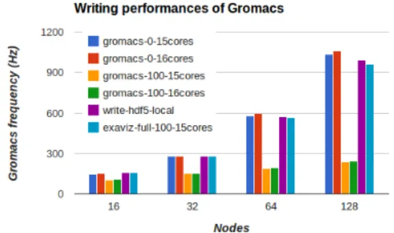
Figure 4. Gromacs frequency when running with various data saving patterns and number of cores.

visible and save atom positions every 100 iteration. Gromacs dynamically balances its work load based on performance measurements. This process can create important frequency jitters for the first 1000 steps. We thus start the timings at the 2000th frame up to the end of the simulation to avoid the perturbations from the initialization phase. We ran the simulations for 5min representing at least 20000 steps.

Figure-4 shows Gromacs running frequency for

vari-ous configurations. The curve Gromacs-0-16cores (resp.

Gromacs-0-15cores) gives the performance of Gromacs run-ning on all the 16 cores available per node (resp. 15 cores) and without performing any IO. These set the performance upper bounds we should try to stay close to when activating data saving. When Gromacs writes to disk the atom positions every 100 steps the performance drops significantly (curve

Gromacs-100-16cores). Adding cores beyond the first 512 ones, does not lead to any additional performance gain.

Next we use FlowVR to gather all data on one helper core per node and locally write one file per node in HDF5

format (curvewrite-hdf5-local). The simulation runs on 15

cores per node and the FlowVR processes (daemon, merge and writer modules) are hosted on a dedicated helper core. At each output step, the atom positions are extracted from the simulation, gathered on each node (no copy) with a merge module and sent (no copy) to a node-local HDF5 writer module. The obtained numbers are very close to

Gromacs-0-15cores, 3.6% slower for 1920 cores, showing the low overhead of the code instrumentation, efficiency of the daemon for coordinating the modules and handling the message transfers.

The last experiment reproduces Gromacs file writing

pat-tern with FlowVR (curvewrite-xtc-merge). Data are gathered

on the master node with a N-To-1 pattern and written

in an XTC file with the Gromacs trjconv tool modified

as described in section IV-A. Transferring the data

asyn-chronously enables to outperform Gromacs-100-16cores,

even though Gromacs uses less cores. Despite the transfer of data, the performance is slightly impacted with a maximum

cost of 6.5%. This is made possible because of the good

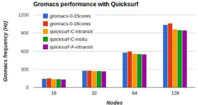
Figure 5. Gromacs frequency when running concurrently with the Quicksurf pipeline.

layer and a fast network interconnection.

Notice that the helper core is never loaded beyond 10% for all these experiments. Therefore, there are opportunities to run extra in situ processings, like data filtering, to make this core more profitable. As we are not using busy wait in the daemon, the user is free to use these cores for running external analytics codes, which may be part of the global FlowVR application or not. Moreover, Gromacs has difficulties to take fully benefits from the 16 cores (except for 64 nodes) motivating the use of a dedicated core.

C. Live Quicksurf

We benchmark several placement strategies, in-situ and in-transit schemes to compute a live Quicksurf based on section IV-B scenarios. The water and ion particles are filtered out in-situ to keep only the lipids. About 30% of the atoms remain after this filtering step. At the end of the pipeline, the partial meshes produced by the marching cube modules are merged to a single visualization node.

Figure-5 compares three configurations with the base

Gromacs performances (Gromacs-0-15cores and

Gromacs-0-16cores).

The quicksurf-c-intransit scenario adopts the the distri-bution strategy (c) of Figure-2 with one helper core per

simulation node, and aNxM redistribution sending the data

to staging nodes . We use one extra staging nodes every 64 simulation nodes. This strategy gives the best performance impacting Gromacs performance decreases by at most 7%

compared to over Gromacs executed without I/O, onNnodes

at 15 cores per node (Gromacs-0-15cores). This strategy

is the lightest regarding network traffic. The global grid represents only 700000 cells and only the non nul densities are sent to the staging nodes.

Thequicksurf-c-insitu scenario also relies on strategy (c) but the redistribution is performed between the simulation

nodes (M =N). The impact on Gromacs is at most 8%

compared to Gromacs-0-15cores. This is higher than for

quicksurf-c-intransit but requires 1.5% less nodes (no stag-ing nodes are used).

Finally, the quicksurf-a-intransit strategy gives a

max-imum cost of 8.6% compared to Gromacs-0-15cores. In

this case the atom positions are directly redistributed to the

staging nodes (M=N/64 staging nodes). The performance

impact is more significant than forquicksurf-c-intransit. This overhead can be explained by the amount of data to transfer (atom positions versus cell densities), which is at least 3 times larger. Even if this strategy is the slowest one, it has the advantage of distributing the atom positions across the staging nodes. These positions are the base data required by a large variety of analysis. The range of possible analysis is significantly more limited if only densities reach the staging nodes as for the 2 other scenarios. This third scenario can thus be more interesting depending on the user needs.

We choose not to place the redistribution component in (b) since it generates more network traffic than in (a) whereas the computational cost to generate the grid is relatively low and can easily be computed after the redistribution.

D. Discussion

The molecular dynamics simulation we rely on departs from the type of simulations usually used to benchmark other in-situ frameworks like [24] or [37]. Molecular dy-namics simulations are characterizer by high frequencies (up to 1061Hz in our case) compared to simulations runnings in between 1Hz and 1/20Hz. The amount of data produced at each output step is inversely proportional to the frequency. Our benchmark produces about 25MB per output step to be compared to the 700 MB reported in [1]. If we normalize the amount of data extracted per node we get a traffic of 2MB per node per second in our case (Gromacs running at 1061Hz on 128 nodes and one output step every 100 steps). In[20], the GTC simulation running on 16,384 cores (2048 nodes) produces 260GB every 2 minutes. It represents a traffic of about 1MB per node per second. Even if a direct comparison is delicate given the very different contexts, we can see that the extracted data exert a similar pressure on the network bandwidth, but in our case at a higher frequency.

Finally, Gromacs uses a dynamic load-balancing system that adapts the grid configuration at runtime. This prevents us to use a priori data-aware redistribution on the simulation nodes like in [30]. Even though the data redistribution towards staging nodes is not impacted by this mechanism, the full in-situ scenario could certainly take advantage of this information.

VI. CONCLUSION

We introduced a dataflow oriented framework for in situ and in transit analytics. Based on the FlowVR middleware, our framework enables to support a large range of scenarios. A Python script describes the assembly of the application, offering the ability to program and reuse advanced patterns. Often a new scenario can be experimented simply by updat-ing the Python script, without module recompilation. The runtime takes care of the application deployment, module coordination and data exchanges, with various levels of

optimization. Because we tried to make FlowVR as inun-trusive as possible (simple module API, direct access to shared memory, module started with their native launching commands), the user keeps a strong control and good understanding of the application behavior.

Experiments with Gromacs molecular simulations paral-lelized on up to 2048 cores, show that our framework enables to concurrently perform analytics with a low impact on the simulation (less than 9%).

So far, we rely on very basic mechanisms to keep the simulation running when errors occur on the analytics pipe-line. Future works include the integration of more advanced fault tolerance mechanisms. On the performance side we will investigate scheduling algorithms to let in-situ processes communicate over the network when not used by the simula-tion. We are also involved in a long-term collaboration with computational biologists to test and develop new scenarios and usages, so in situ processing can become part of their standard software toolbox.

ACKNOWLEDGMENTS

This work was partly funded by the ANR, project EXAVIS ANR-11-MONU-003. Most of the computations presented in this paper were performed using the Froggy platform of the CIMENT infrastructure (https://ciment.ujf-grenoble.fr), supported by the Rhˆone-Alpes region (GRANT CPER07 13 CIRA) and the Equip@Meso project (reference ANR-10-EQPX-29-01) of the programme Investissements d’Avenir supervised by the ANR. We thank Jeremy Jaus-saud, INRIA, and Pierre Neyron, CNRS, for their helpful inputs and contributions. We thank Philip Fowler, University of Oxford, for his expertise on Gromacs scalability.

REFERENCES

[1] G. Zhao, J. R. Perilla, E. L. Yufenyuy, X. Meng, B. Chen, J. Ning, J. Ahn, A. M. Gronenborn, K. Schulten, and C. Aiken, “Mature HIV-1 Capsid Structure by Cryo-electron Microscopy and All-Atom Molecular Dynamics,” pp. 643– 646, 2013.

[2] H. Yu, C. Wang, R. Grout, J. Chen, and K.-L. Ma, “In situ visualization for large-scale combustion simulations,”

Computer Graphics and Applications, IEEE, vol. 30, no. 3, pp. 45–57, 2010.

[3] W. Gu, G. Eisenhauer, K. Schwan, and J. Vetter, “Falcon: On-line monitoring for steering parallel programs,” in In Ninth International Conference on Parallel and Distributed Computing and Systems (PDCS’97), 1998, pp. 699–736. [4] J. C. Bennett, H. Abbasi, P.-T. Bremer, R. Grout, A. Gyulassy,

T. Jin, S. Klasky, H. Kolla, M. Parashar, V. Pascucci, P. Pebay, D. Thompson, H. Yu, F. Zhang, and J. Chen, “Combining in-situ and in-transit processing to enable extreme-scale sci-entific analysis,” innternational Conference on High Perfor-mance Computing, Networking, Storage and Analysis. IEEE Computer Society Press, 2012, pp. 49:1–49:9.

[5] S. Pronk, S. Pall, R. Schulz, P. Larsson, P. Bjelkmar, R. Apos-tolov, M. R. Shirts, J. C. Smith, P. M. Kasson, D. van der Spoel, B. Hess, and E. Lindahl, “Gromacs 4.5: a high-throughput and highly parallel open source molecular sim-ulation toolkit,”Bioinformatics, vol. 29, no. 7, pp. 845–854, 2013.

[6] M. Krone, J. E. Stone, T. Ertl, and K. Schulten, “Fast Visualization of Gaussian Density Surfaces for Molecular Dynamics and Particle System Trajectories,” inEuroVis 2012 Short Papers, vol. 1, 2012, pp. 67–71.

[7] N. Fabian, K. Moreland, D. Thompson, A. Bauer, P. Mar-ion, B. Geveci, M. Rasquin, and K. Jansen, “The Paraview Coprocessing Library: A Scalable, General Purpose In Situ Visualization Library,” inLarge Data Analysis and Visualiza-tion (LDAV), 2011 IEEE Symposium on, 2011, pp. 89–96. [8] B. Whitlock, J. M. Favre, and J. S. Meredith, “Parallel In

Situ Coupling of Simulation with a Fully Featured Visual-ization System,” in11th Eurographics conference on Parallel Graphics and Visualization, 2011, pp. 101–109.

[9] benjamin Lorendeau, Y. Fournier, and A. Ribes, “In Situ vi-sualization in fluid mechanics using Catalyst: a case study for Code Saturne,” inIEEE Symposium on Large Data Analysis and Visualization (LDAV), 2013.

[10] M. Dorier, G. Antoniu, F. Cappello, M. Snir, and L. Orf, “Damaris: How to Efficiently Leverage Multicore Parallelism to Achieve Scalable, Jitter-free I/O,” in CLUSTER - IEEE International Conference on Cluster Computing. IEEE, Sep. 2012.

[11] M. Li, S. S. Vazhkudai, A. R. Butt, F. Meng, X. Ma, Y. Kim, C. Engelmann, and G. Shipman, “Functional partitioning to optimize end-to-end performance on many-core architec-tures,” in International Conference for High Performance Computing, Networking, Storage and Analysis, 2010, pp. 1– 12.

[12] A. Singh, P. Balaji, and W.-c. Feng, “GePSeA: A General-Purpose Software Acceleration Framework for Lightweight Task Offloading,” in International Conference on Parallel Processing, 2009, pp. 261–268.

[13] X. Ma, J. Lee, and M. Winslett, “High-Level Buffering for Hiding Periodic Output Cost in Scientific Simulations,” Par-allel and Distributed Systems, IEEE Transactions on, vol. 17, no. 3, pp. 193–204, 2006.

[14] J. Biddiscombe, J. Soumagne, G. Oger, D. Guibert, and J.-G. Piccinali, “Parallel Computational Steering and Analysis for HPC Applications using a ParaView Interface and the HDF5 DSM Virtual File Driver,” in Eurographics Symposium on Parallel Graphics and Visualization, T. Kuhlen, R. Pajarola, and K. Zhou, Eds., 2011, pp. 91–100, honourable Mention Award.

[15] T. Tu, C. A. Rendleman, D. W. Borhani, R. O. Dror, J. Gullingsrud, M. O. Jensen, J. L. Klepeis, P. Maragakis, P. Miller, K. A. Stafford, and D. E. Shaw, “A Scalable Parallel Framework for Analyzing Terascale Molecular Dynamics Simulation Trajectories,” in Conference on Supercomputing, 2008, pp. 56:1–56:12.

[16] E. Deelman, G. Singh, M.-H. Su, J. Blythe, Y. Gil, C. Kessel-man, G. Mehta, K. Vahi, G. B. BerriKessel-man, J. Good, A. Laity, J. C. Jacob, and D. S. Katz, “Pegasus: A Framework for Mapping Complex Scientific Workflows onto Distributed Sys-tems,”Sci. Program., vol. 13, no. 3, pp. 219–237, Jul. 2005. [17] B. Lud¨ascher, I. Altintas, C. Berkley, D. Higgins, E. Jaeger, M. Jones, E. A. Lee, J. Tao, and Y. Zhao, “Scientific Workflow Management and the Kepler System: Research Articles,”

Concurr. Comput. : Pract. Exper., vol. 18, no. 10, pp. 1039– 1065, Aug. 2006.

[18] C. Docan, M. Parashar, and S. Klasky, “DataSpaces: an Inter-action and Coordination Framework forCoupled Simulation Workflows,”Cluster Computing, vol. 15, no. 2, pp. 163–181, 2012.

[19] H. Abbasi, G. Eisenhauer, M. Wolf, K. Schwan, and S. Klasky, “Just in Time: Adding Value to the IO Pipelines of High Performance Applications with JITStaging,” in Interna-tional symposium on High performance distributed comput-ing, 2011, pp. 27–36.

[20] F. Zheng, H. Abbasi, C. Docan, J. Lofstead, Q. Liu, S. Klasky, M. Parashar, N. Podhorszki, K. Schwan, and M. Wolf, “Pre-DatA - Preparatory Data Analytics on Peta-Scale Machines,” in Parallel Distributed Processing (IPDPS), 2010 IEEE In-ternational Symposium on, 2010, pp. 1–12.

[21] J. C. Bennett, H. Abbasi, P.-T. Bremer, R. Grout, A. Gyulassy, T. Jin, S. Klasky, H. Kolla, M. Parashar, V. Pascucci, P. Pebay, D. Thompson, H. Yu, F. Zhang, and J. Chen, “Combining In-Situ and In-Transit Processing to Enable Extreme-Scale Scientific Analysis,” in Conference on High Performance Computing, Networking, Storage and Analysis, 2012, pp. 49:1–49:9.

[22] C. Docan, M. Parashar, and S. Klasky, “Dart: a substrate for high speed asynchronous data io,” in17th international sym-posium on High performance distributed computing, 2008, pp. 219–220.

[23] J. F. Lofstead, S. Klasky, K. Schwan, N. Podhorszki, and C. Jin, “Flexible io and integration for scientific codes through the adaptable io system (adios),” in6th international workshop on Challenges of large applications in distributed environments, 2008, pp. 15–24.

[24] F. Zheng, H. Zou, G. Eisnhauer, K. Schwan, M. Wolf, J. Dayal, T. A. Nguyen, J. Cao, H. Abbasi, S. Klasky, N. Podhorszki, and H. Yu, “FlexIO: I/O middleware for Location-Flexible Scientific Data Analytics,” in IPDPS’13, 2013.

[25] F. Bertrand, R. Bramley, A. Sussman, D. E. Bernholdt, J. A. Kohl, J. W. Larson, and K. B. Damevski, “Data Redistribution and Remote Method Invocation in Parallel Component Archi-tectures,” in19th IEEE International Parallel and Distributed Processing Symposium (IPDPS’05), 2005.

[26] J.-Y. Lee and A. Sussman, “High Performance Communi-cation Between Parallel Programs,” inInternational Parallel and Distributed Processing Symposium (IPDPS’05), 2005.

[27] G. Edjlali, A. Sussman, and J. H. Saltz, “Interoperability of Data Parallel Runtime Libraries,” in 11th International Symposium on Parallel Processing, 1997, pp. 451–459. [28] K. Keahey, “PAWS: Collective Interactions and Data

Trans-fers,” in High Performance Distributed Computing Confer-ence, 2001, pp. 47–54.

[29] H. Abbasi, M. Wolf, K. Schwan, G. Eisenhauer, and A. Hilton, “XChange: Coupling Parallel Applications in a Dynamic Environment,” inIEEE International Conference on Cluster Computing, 2004.

[30] F. Zhang, C. Docan, M. Parashar, S. Klasky, N. Podhorszki, and H. Abbasi, “Enabling In-situ Execution of Coupled Scientific Workflow on Multi-core Platform,” in Parallel Distributed Processing Symposium (IPDPS), 2012, pp. 1352– 1363.

[31] J. Allard, J.-D. Lesage, and B. Raffin, “Modularity for Large Virtual Reality Applications,” Presence: Teleoperators and Virtual Environments, vol. 19, no. 2, pp. 142–162, April 2010. [32] B. Hess, C. Kutzner, D. van der Spoel, and E. Lindahl, “GRO-MACS 4: Algorithms for Highly Efficient, Load-Balanced, and Scalable Molecular Simulation,” Journal of Chemical Theory and Computation, vol. 4, no. 3, pp. 435–447, 2008. [33] M. Dreher, P. Marc, T. Ahmed, C. Matthieu, M. Baaden,

N. F´erey, S. Limet, B. Raffin, and S. Robert, “Interactive Molecular Dynamics: Scaling up to Large Systems,” in Inter-national Conference on Computational Science, ICCS 2013. Elsevier, Jun. 2013.

[34] N. Michaud-Agrawal, E. J. Denning, T. B. Woolf, and O. Beckstein, “Mdanalysis: A toolkit for the analysis of molecular dynamics simulations,”J. Comput. Chem., vol. 32, pp. 2319–2327, 2011.

[35] H. Yu, C. Wang, and K.-L. Ma, “Massively parallel volume rendering using 2-3 swap image compositing,” inACM/IEEE conference on Supercomputing (SC’08), 2008, pp. 48:1– 48:11.

[36] [Online]. Available: http://philipwfowler.wordpress.com/2013/10/23/gromacs-4-6-scaling-of-a-very-large-coarse-grained-system/

[37] M. Dorier, R. Sisneros, T. Peterka, G. Antoniu, and D. Se-meraro, “Damaris/Viz: a Nonintrusive, Adaptable and User-Friendly In Situ Visualization Framework,” inIEEE Sympo-sium on Large Data Analysis and Visualization (LDAV), 2013.