Date of publication xxxx 00, 0000, date of current version xxxx 00, 0000.
Digital Object Identifier 10.1109/ACCESS.2017.Doi Number
Multipath Estimation Based on Modified
ε-constrained Rank-based Differential Evolution
with Minimum Error Entropy
Lan Cheng 1, Member, IEEE, Hong Yue 2, Senior Member, IEEE, Yanjun. Xing 3, Mifeng Ren 1, Member, IEEE
1Taiyuan University of Technology, Taiyuan 030024, China
2Department of Electronic and Electrical Engineering, University of Strathclyde, GlasgowG1 1XW, UK 3China Unicom Ltd, Taiyuan 030001, China
Corresponding author: Lan Cheng ([email protected]).
This work was supported in part by the National Natural Science Foundation of China under Grant 61503271 and Grant 61603267 and in part by the China Scholarship Council under Grant 201606935041.
ABSTRACT Multipath is one of the dominant error sources for high-precision positioning systems, such as global navigation satellite systems (GNSS). The minimum mean square error (MSE) criterion is usually employed for multipath estimation under the assumption of Gaussian noise. For non-Gaussian noise as appeared in most practical applications, alternative solutions are required for multipath estimation. In this work, a multipath estimation algorithm is proposed based on the minimum error entropy (MEE) criterion under Gaussian or non-Gaussian noises. A key advantage of using MEE is that it can minimize the randomness of error signals, however, the shift-invariance characteristics in MEE may lead to a bias of the estimation result. To mitigate such a bias, an improved estimation strategy is proposed by integrating the second-order central moment of the estimation error together with the prior information of multipath parameters as a constraint. The multipath estimation problem is thus formulated as a constrained optimization problem. A modified ε-constrained rank-based differential evolution (εRDE) algorithm is developed to find the optimal solution. The effectiveness of the proposed algorithm, in terms of reducing the multipath estimation error and minimizing the randomness in the error signal, has been examined through case studies with Gaussian and non-Gaussian noises.
INDEX TERMS Multipath estimation, constrained optimization, mean square error (MSE), minimum error entropy (MEE), ε- constrained rank-based differential evolution (εRDE).
I. INTRODUCTION
Multipath, the delayed replica of direct signal caused by the reflection of buildings, hills and other obstacles, cannot be eliminated by differential techniques due to the irrelevancy between different instants and the uncertain occurrence along the observation period. Thus, multipath has become one of the dominant error sources degrading the positioning accuracy in differential positioning systems [1-3]. In the presence of multipath, the direct signal and the multipath signal contained in the composite signal, tracked by a receiver, cannot be distinguished from each other. As a result, an error arises, which is known as multipath error.
Various methods have been developed to mitigate the multipath error, such as the antenna techniques in front, the correlator and discriminator-based methods in delay lock
since the statistical property of the target state can be fully determined by the two parameters [13]. Other algorithms developed on data processing, such as the multipath interference mitigation algorithm based on WRELAX, the methods based on spatial domain decoupled parameter estimation theory, are also used to mitigate multipath error, and the performance of these algorithms are comprehensively analyzed in [14]. However, only Gaussian noises are considered in these algorithms.
For systems with non-Gaussian noise, the estimation performance of the aforementioned algorithms is likely to deteriorate since higher order statistical properties are often required to describe the non-Gaussian characteristics of the target state. The estimation performance can also degrade even for Gaussian noise if the system is non-linear because the target state variable may not be Gaussian distributed due to the system nonlinearity [15]. Thus, considering only the mean and variance would be insufficient in characterizing nonlinear and/or non-Gaussian processes.
A target state can be fully characterized by the shape of its probability density function (PDF). In this regard, it is beneficial to consider the entire PDF of the state rather than its low order moments [16]. The particle filter (PF) algorithms have been used for multipath estimation for its applications to general noise situations [17]. Here the PF is in principle a Bayesian estimation for a given measurement sequence. It can also be taken as a PDF estimation since a number of particles are used to represent the distribution of the state. However, the problems of sample degeneration and impoverishment restrict the applications of PF algorithms [18].
The PDF-shaping control methodology has been developed and applied to control systems with non-Gaussian noise and nonlinear dynamics [19, 20]. An alternative measure for general non-Gaussian systems is the entropy, which is a scalar quantity in information theory that quantifies the average uncertainty involved in a random variable [21]. Entropy can be used to depict the higher-order statistics of a distribution since it is formulated on the PDF. The use of entropy is not limited to Gaussian assumption. Thus, the so-called minimum error entropy (MEE) criterion has been employed in many stochastic distribution control problems [22-24].
The MEE criterion is a shift-invariant measure, which means the mean of the error can be a non-zero value even when the entropy measure is minimized. To deal with this problem, a constraint on zero mean of the estimation error is added to the MEE performance index in some algorithms [15, 25]. In our previous work, an algorithm based on the central error entropy criterion (CEEC) is proposed for multipath estimation [26], which can reduce the mean error but appears to be sensitive to the initial states and the initial gain matrix in the filter design. With the MEE-based state estimation methods, it is usually assumed that the noise PDF is known, which could be impractical for many applications [22]. Several data-driven methods have been developed for
systems with unknown noise PDF [23, 24].
Stochastic information gradient (SIG) method is often applied to update the filter gain in the design of a sub-optimal estimator. The drawbacks of using SIG are considered as follows. (1) It cannot guarantee a global optimum result. (2) Partial derivative operations are required in implementing the searching, which is not a trivial task numerically, especially for high-dimension systems [27].
In this work, the performance index of MEE is taken as the objective function. The second-order central moment of the estimation error, together with the prior parameter information, is formed as a constraint. The prior parameter information is often used in EKF-based or PF-based methods for generation of the initial state. In this new algorithm, the prior information is considered in the constraints rather than in the objective function as in [15]. As such, the multipath estimation is formulated as a constrained optimization problem. An intelligent optimization algorithm, instead of a SIG-based method, is tailored to find the global optimum. This makes a novel contribution to multipath estimation for general stochastic systems.
The remainder of this paper is organized as follows. The signal model and the system model in multipath environments are introduced in Section II. In Section III, the multipath estimation problem is formulated as a constrained optimization problem. A modified recursive ε-constrained rank-based differential evolution (εRDE) algorithm is developed to find the optimum solution in Section IV. Simulation studies for single multipath and two multipaths cases with Gaussian and non-Gaussian noises are reported in Section V. Conclusions and the future work are discussed in Section VI.
II. PROBLEM FORMULATION
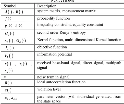
[image:2.576.296.539.522.726.2]For the convenience of reading, notations used in this paper are defined in Table I. For a variable x, we use x to represent its prediction and xˆ to represent the estimation or the filter result.
TABLE I NOTATIONS Symbol Description
( )⋅
A , B( )⋅ system matrix, measurement matrix
( )
f ⋅ probability function ( )
j
g ⋅ ,hj( )⋅ inequality constraint, equality constraint ( )
2
H ⋅ second-order Renyi’s entropy ( )
δ
κ ⋅ ,GΣ( )⋅ Kernel function, multi-dimensional Kernel function
( )
k
J ⋅ objective function
( )
k
V ⋅ information potential ( )
r ⋅ , rd( )⋅ ,
( )
m
r ⋅
received base-band signal, direct signal, multipath signal
n noise term in signal ( )
R ⋅ ideal autocorrelation function ( )
ε ⋅ violation level
k
VOLUME XX, 2018 k
y , s k
y , yk p, measurement vector, the s-th element ofyk, the p
-th realization of yk
e e = yk−yk
Σ Kernel parameter matrix
0,k
α ,αm k, direct signal amplitude, m-th multipath amplitude 0,k
l ,lm k, time delays of the direct signal and the m-th multipath
0,k
θ ,
,
m k
θ direct signal phase, m-th multipath time delay relative to the direct signal
p
ϕ constraint of the p-th individual
0.k
A ,Am k. composite amplitudes of the direct signal and the m -th multipa-th
s
d spacing between the s-th correlator and the punctual correlator
M multipath number S correlator number
𝑇𝑇𝑐𝑐𝑐𝑐𝑐𝑐, 𝑐𝑐𝑐𝑐 parameters in modified εRDE algorithm
𝛿𝛿𝑠𝑠2 variance of the s-th element in e
p
N ,W population size, length of the Parzen window p
F ,CRp,
max
EF
scale factor, crossover rate, maximum evolution number
A. SIGNAL DESCRIPTION
In a global navigation satellite system (GNSS), the received signal in the presence of multipath, 𝑟𝑟(𝑖𝑖), can be described by an (M+1)- path model composed of a direct path signal,
( )
dr i , and the M reflected signals, rm
( )
i , plus the noisetermn i
( )
. Assume that the frequency tracking has been realized by a frequency lock loop, then, the corresponding base-band signal at an in-phase channel at instant i can be modeled as( )
(
) ( )
( )
(
) (
)
( )
( )
d
m
0, 0, 0,
, 0, , 0, ,
1
- cos
- - cos
k k k
r i M
m k k m k k m k
m
r i
r i c i l
c i l l n i
α θ
α θ θ
=
=
+
∑
+ +
(1)
where 𝛼𝛼0,𝑘𝑘 and 𝛼𝛼𝑚𝑚,𝑘𝑘 are the amplitude of the direct signal and the amplitude of the m-th multipath reflected signal. 𝑙𝑙0,𝑘𝑘 and 𝑙𝑙𝑚𝑚.𝑘𝑘 are time delays of the direct signal and the m-th multipath signal. 𝑐𝑐(𝑖𝑖 − 𝑙𝑙0,𝑘𝑘) and 𝑐𝑐(𝑖𝑖 − 𝑙𝑙0,𝑘𝑘− 𝑙𝑙𝑚𝑚,𝑘𝑘) are the pseudo code with delay 𝑙𝑙0,𝑘𝑘and(𝑙𝑙0,𝑘𝑘−𝑙𝑙𝑚𝑚,𝑘𝑘) . 𝜃𝜃0,𝑘𝑘 and 𝜃𝜃𝑚𝑚,𝑘𝑘
are direct signal phase and the m-th multipath time delay relative to the direct signal. The signal model in (1) is a simplified version of the model adopted in [28] and more details can be found in [29]. For the model in this work, the real part of the complex base-band signal is obtained from the in-phase channels as in [30], and the imaginary part can be obtained through orthogonal channels.
Although there are some other signal models, for example, the multipath model in urban canyon [31], which mainly concerns the multipath caused by the motion of satellite, we still adopt the model expressed by (1) not only because it’s widely used but also because the multipath caused by the
motion of satellite can also be described by (1) as well as the motion of receiver.
B. SYSTEM MODEL
The initial values of lˆ0,k, lˆ0,0, can be obtained from the capture stage. The structure of signal tracking in GNSS is shown in Fig. 1. The measurement vector,
T 1 2
,
,
,
S k=
y y
k ky
k
y
, can be obtained by correlating the received signal, r i( )
, with the local C/A code vector over the measurement period. d is the correlator spacing vector with d=[
d d1, 2,,ds]
T, s=1, 2, …, S, S is the correlator number. c i l(
−ˆ0,k+ds)
is the s-th local code, ds >0 [image:3.576.301.540.277.389.2]corresponds to the early code, ds <0 corresponds to the late code and ds =0 refers to the punctual code.
FIGURE 1. Structure of signal tracking scheme
The multipath parameters to be estimated can be grouped into a vector as
T 0, , 1, , , , , 0, , 1, , , , ,0, ,1, , , ,
k = α αk k αM k θ θk k θM k l k l k lM k
x .
k
x can be estimated according to yk if enough correlator
outputs are available [28]. Then, the multipath part, rm
( )
k , can be reconstructed according to the estimate of xk, and the direct signal can be obtained by subtracting the multipath part from the received signal. The estimated time delay at the next observation period, lˆ0,k+1, can then be calculated so asto tune the local code generator to synchronize the punctual code with the received signal.
[image:3.576.299.524.624.692.2]The relationship between the i-th instant corresponding to one sample interval Ts and the k-th measurement corresponding to one measurement period To can be illustrated in Fig. 2.
The output of the s-th correlator in Fig. 1 is
(
)
( )
(
)
(
)
(
)
( ) o s0, , 0, ,
0, / 1
o s
0, , ,
1 , , , , 1 ˆ / k k k s
k m k k m k
kK
k s
i kK T T
M
k k s m k k m k s k
m
y A A l l
r i c i l d
T T
A R γ d A R γ l d n
= − + = , = ⋅ − + = − + − − +
∑
∑
x B x (2)where γk =lˆ0,k−l0,k , A0,k =α0,kcos
( )
θ0,k and(
)
, , cos 0, ,
m k m k k m k
A =α θ +θ .
o s
K=T T . B
( )
⋅ is the measurement matrix with the following form.( )
0,(
)
,(
,)
1
M
k k k s m k k m k s
m
A R γ d A R γ l d
=
= − +
∑
− −B x (3)
( )
R ⋅ is the ideal autocorrelation function with the following form.
( )
(
)
(
)
o s o s 0, 0, / 1 c 1 /1 , 1
0, otherwise
ˆ
kK
k k k
i kK T T
k k
R c
T T
T
i l c i l
γ γ γ = − + = − ≤ ≈ − ⋅ −
∑
(4)
where Tc =1/1023 ms for GPS signal, 1023 is the number of C/A code chips in a period.
It can be seen from (2) that the parameters to be estimated at the k-th measurement are grouped into
T 0, , 1, , , , ,0, ,1, , , ,
k= Ak Ak AM k l k l k lM k x
based on the assumption that the phase delay is not changed during the observation period, and the phase estimation can be obtained as in [30]. Here
(
Q I)
0,k arctan Am k, Am k,
θ = (5) where Am kI, and Am kQ, are the estimated amplitudes from the in-phase channels and the quadrature channels.
Assume xk can be formulated as a first-order Markov process, i.e.
(
1)
k = k− + k
x A x w (6)
( )
k = k + k
y B x v (7) where k D1
× ∈
x denotes the state vectors, D=2
(
M+1)
.k
w is assumed to be Gaussian distributed noise with zero mean and the covariance matrix Q. yk∈S×1 is the
measurement vector with 1 2 T
, , , S
k = yk yk yk
y and
y
ksisobtained according to (2). vkis the measurement noise with zero mean and it can be Gaussian distributed or non-Gaussian distributed. A and B are system matrix and measurement matrix of appropriate dimensions.
In this work, it is aimed to recursively estimate xk
according to the observation vector, yk. Here, yk =B x
( )
k , kx is the prediction result of xk that can be obtained from
(6) by setting an initial state. The prediction of yk, rather
than the filter result of yk , is used to construct the
measurement error. In this case the gain matrix appeared in traditional filter is not required. In fact, ek=yk−yk, which
is called innovation in Kalman filter-based methods, is used to update the filter result, xˆk, in the sense of the MEE and the constraint.
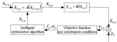
[image:4.576.299.536.232.317.2]The main idea is to update the filter result using an intelligent algorithm. Then, the above estimation problem can be formulated as an optimization problem with the MEE criterion. The prior information of multipath and other useful information can be combined as constraints. The structure of this estimation strategy is demonstrated in Fig. 3.
FIGURE 3. The structure of the estimator based on intelligent optimization algorithm
If the range of xk is given according to the prior
information of multipath, 𝑁𝑁𝑝𝑝 individuals can be generated uniformly distributed in this range and they are grouped as the initial population, p=1, 2,,Np . ek p, =yk−yk p, . fp
and
ϕ
p are the objective function and the constraint of the p-th individual, respectively, which will be explained in Section III in detail.
III. CONSTRAINED OPTIMIZATION PROBLEM OF
MULTIPATH ESTIMATION
In this section, the multipath estimation is formulated as a constrained optimization problem. The objective function, the constraint and the boundary conditions are discussed.
A. OBJECTIVE FUNCTION DESIGN
Entropy is an index to measure uncertainty and randomness of a general stochastic variable. The MEE estimation aims to minimize the entropy of the estimation error, and hence decrease the uncertainty in estimation. Assume a random variable e has PDF f e
( )
, the second-order Renyi’s entropy is defined by [32]( )
2( )
2 log d
H e = −
∫
f e e (8) For a vector e with S dimension, the kernel density estimation (KDE) can be used to estimate its PDF. Given a set of independent and identically distributed (i.i.d.) data,{ }
1N i i=
e , drawn from a distribution, the KDE of the PDF is
( )
(
)
1 1 ˆ N i i f G N ==
∑
Σ −VOLUME XX, 2018
with N being the number of samples and Σ the kernel parameter matrix. GΣ
(
e e− i)
is a multi-dimensional Gaussian function with the form as follows.(
)
( )
( )
(
)
(
)
T 1 1 1 exp 2 2 deti S i i
G π − − = − − −
Σ e e e e Σ e e
Σ
(10)
Σ is assumed to be a diagonal matrix with the s-th diagonal element being the variance
δ
s2 for es in e. Σ−1is the inversematrix of Σ . A large number of experiments show that once
δ
s2 is larger than a certain value it has little influence on the estimation results.Using KDE, the Renyi’s quadratic entropy can be formulated as follows.
( )
(
)
(
)
(
)
(
)
(
)
(
)
( )
2 2 1 2 1 1 2 1 1 2 2 1 1 1 log d 1 log d 1 log d 1 log = log N i i N N i j i j N N i j i j N N i j i j H G N G G N G G N G N V = = = = = = = = − − = − − − = − − − = − − −∑
∫
∑∑
∫
∑∑∫
∑∑
Σ Σ Σ Σ Σ Σe e e e
e e e e e
e e e e e
e e
e
(11)
where
( )
2 2(
)
1 1
1 N N
i j
i j
V G
N = =
= −
∑∑
Σ e e e (12) is called the information potential (IP) of e andΣ2 = 2Σ. Thus, minimizing the Renyi’s entropy, H2
( )
e , isequivalent to maximizing the IP, V e
( )
, because of the monotonic property of the log( )
⋅ function. In order to reduce the calculation complexity, the instantaneous information potential, V ek( )
, instead of V e( )
, is used, i.e.,( )
2(
)
1
1
N i k k iV
G
N
= =
∑
Σ−
e
e
e
(13) The calculation of V ek( )
can be further simplified with theParzen windowing technique as
( )
2(
)
1
1
ki
k k
i k W
V
G
W
= − +
=
∑
Σ−
e
e
e
(14) where W is the length of the Parzen window.Given that e e1, ,2 eS are independent of each other,
( )
k
V e can be written as
( )
(
)
(
)
2 2, +1 +1 11
1
s k i k ki k W S k
s s
i k i k W s
V
G
W
e
e
W
κ
δ= − = − =
=
−
=
−
∑
∑ ∏
Σe
e
e
(15)
where
( )
(
)
(
2 2)
1 2 exp 2
e e
δ
κ = π δ δ is a Gaussian kernel
function. Thus,V ek
( )
needs to be maximized in order to minimize the randomness of the estimation error. Then, the maximization problem can be transformed into a minimization problem by taking the following objective function.( )
( )
k k
J
e = -
V
e
(16) The objective function in (16) is used for multipath estimation.B. CONSTRAINTS
Due to the shift-variant property of MEE, the following constraint is considered to minimize the mean error.
( )
min E e eT(17) Here E(∙) is the expectation function. In order to reduce the calculation complexity, E
( )
e eT is calculated by thefollowing statistical information
( )
T( )
T1
1 E
k
i i
i k W
W = − +
=
∑
e e e e (18)
where W is the same window length as in (15).
In order to control the estimation accuracy, a threshold is introduced to convert (18) into an equality constraint.
( )
T 11 k
i i i k W
threshold W = − +
∑
e e =(19)
where the threshold is a small positive number, such as
threshold=10-5.
Remark 1W samples are required for calculations in (18). The estimation results from the
(
k W− +1)
-th iteration to thek-th iteration need to be saved for further processing in the recursive procedure.
The multipath signal is normally weaker than the direct signal since some signal power is lost due to reflection. This means the multipath amplitude is smaller than the direct signal amplitude, i.e.
, 0,
m k k
α
<α
(20) with m=1, 2,,M.Without loss of generality, the following assumption is made. The first multipath has the smallest relative time delay, the second multipath has a longer time delay compared to the first one, and so on, that is,
, 1,
m k m k
l <l + (21)
with m+ ≤1 M . Then, the constraints known as the prior information are listed by (19), (20) and (21), which is consistent with that in [10].
C. BOUNDARY CONDITIONS
acquisition process is usually less than 0.5Tc [28], which yields −0.5Tc≤γk ≤0.5Tc. Thirdly, the multipath signal
arrives after the direct signal because it must travel a longer distance over the propagation path, so the multipath time delay is longer than the direct signal time delay, i.e. lm ≥0.
Only the short multipath with time delay of 0≤lm≤2Tc is
considered since the multipath with longer time delay can be ignored owing to the autocorrelation properties of C/A code [30]. Accordingly, the boundary considerations can be given as
0,
0<
α
k ≤1 (22) ,0<
α
m k ≤1 (23)c c
0.5T γk 0.5T
− ≤ ≤ (24)
c
0≤lm≤2T (25) In this way, the multipath estimation problem is converted into a constrained optimization problem with the objective function (18), the constrained conditions in (19) ~ (21), and the boundary conditions in (22) ~ (25). In this optimization problem, the state dimension is 2
(
M+1)
, the number of the equality constraint condition is one, and the number of the non-equality constraint conditions is 2M.In a two-stage estimation algorithm based on variable projection (VP) method, a constraint is used to improve the multipath mitigation performance [33], in which the VP method is designed to correct the pseudo-range error caused by multipath and the constraint is imposed on the multipath-caused range error. Our algorithm in this work is proposed to estimate multipath parameters (multipath amplitude, multipath time delay and multipath phase delay) and the constraints are directly imposed on these parameters. In addition, the VP method is employed to suppress the multipath error after the initial pseudo range is obtained, therefore the proposed algorithm is able to eliminate the multipath error before the multipath influences the pseudo range.
IV. MULTIPATH ESTIMATION BASED ON MODIFIED
εRDE ALGORITHM
The εRDE algorithm was initially proposed in [10] to solve constrained optimization problems with equality constraints. In this work, a modified εRDE algorithm is developed to solve the constrained optimization problem for multipath estimation.
A. CONSTRAINED OPTIMIZATION PROBLEM
A typical constrained optimization problem can be described as follows [10].
Minimize
(
J x( )
)
Subject to
( )
( )
c0, 1, ,
0, 1, ,
, 1, ,
j
j
t t t
g j n
h j n J
L x U t D
≤ =
= = +
≤ ≤ =
x x
(26)
where x=
(
x x1, 2,,xD)
is a D-dimension vector. J x( )
isan objective function. gi
( )
x ≤0 and hj( )
x =0 are qinequality constraints and Jc−n equality constraints, respectively. J
( )
⋅ , gj( )
⋅ , hj( )
⋅ are linear or nonlinear real-valued functions. Lt and Ut are the lower and upper bounds of xt.Lt and Ut are chosen according to the prior information of a particular problem. In this paper, Lt andt
U are set according to the boundary condition in (22) ~ (25). The feasible solution space in which every point can meet all constraints is denoted by Ƒ, and the searching space defined by the upper and lower bounds is denoted by Ş. Apparently, Ƒ⊆Ş.
In the ε-constrained method, the constraint violation,
( )
ϕ
x , can be given by the following formula [10].( )
max 0,{
i( )}
q j( )
qi j
g h
ϕ
x =∑
x +∑
x (27)where q is a positive integer, q=1 is chosen in this paper for the simplification of calculation, which is also the choice in [10]. |∙|means the absolute operation, ‖∙‖ denotes the 2-norm operation. The main idea of the ε-constrained method is to sort the individuals according to a ε-level comparison strategy.The ε-level comparison defines a rank for a given individual by comparing the pair
(
J( ) ( )
x ,ϕ x)
of the given individual and that of other individuals. The rank Rb of the base individual used for the evolution of the p-th individual is adopted to calculate the corresponding scale factor, Fp, and the crossover rate, CRp ,which will be used in the process of differential evolution. More details can be found in [10].Remark 2 The ε-level comparison is a hierarchical sequence comparison method, in which the sorting is performed firstly according to
ϕ
( )
x rather than J x( )
because it is more important to make x be feasible than to minimize J x
( )
.B. MODIFIED εRDE ALGORITHM
VOLUME XX, 2018
statistical property of the estimation error as time goes on. This idea can be realized by adaptively setting the violation level,
ε
( )
k , as follows.( )
( )
concon
con 1
1 1 , 1
0, cp k k T k T k T ε ε −
− < ≤
=
>
(28)
with
ε
( )
1 being the sum of the constraint violation degree of the top a-th individuals. a=0.2Np is chosen in this paper.con
T and cp are constants used to control the convergence speed.
Remark 3 The iteration index k in (28) is used to update the violation level,
ε
( )
k , instead of the evolution number in [10]. This change is made for recursive estimation in this work that needs to consider noise. The violation level will decrease gradually towards zero as the iteration goes on.Denote ϕ1 and ϕ2 as the constraint violations for two
different individuals x1 and x2 . In order to reduce the
complexity of the εRDE algorithm, the case of ϕ1=ϕ2 is not
taken into consideration since it is unlikely to have ϕ1=ϕ2
in practical applications. As a result, the ε-level comparison defined in [10] can be simplified as follows.
(
) (
)
1 2 1 21 1 2 2
1 2
, ,
, ,
otherwise
J J
J ϕ J ϕ ϕ ϕ ε
ϕ ϕ
< ≤
< ⇔
<
(29)
(
) (
)
1 2 1 21 1 2 2
1 2 , ,
, ,
otherwise
J J
J ϕ J ϕ ϕ ϕ ε
ϕ ϕ
≤ ≤
≤ ⇔
≤
(30)
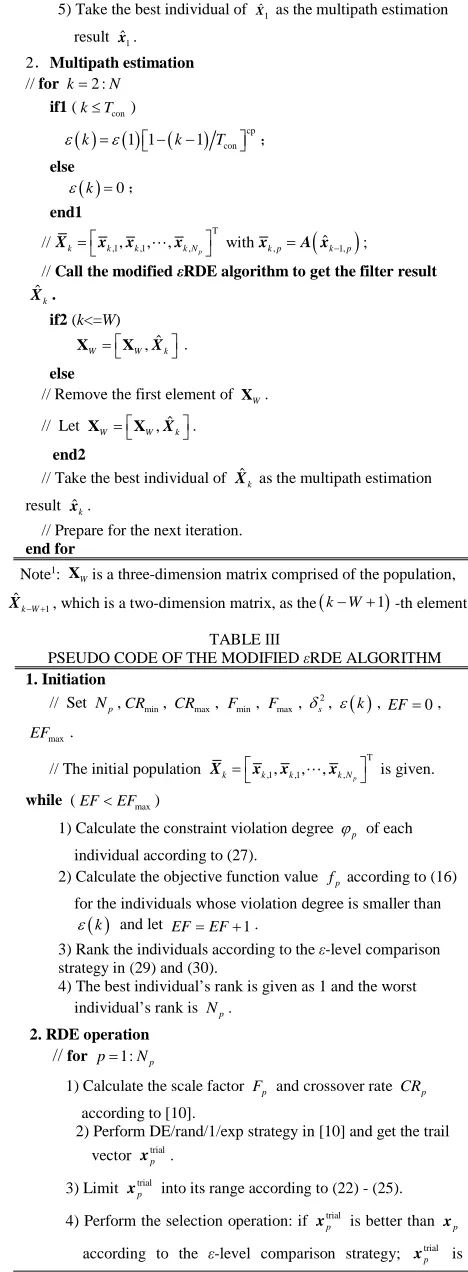
The pseudo code of the proposed multipath estimation algorithm is given in Table Ⅱ. Herein the best individual of a population is chosen as the filter output, xˆk , at each iteration. The pseudo code of the modified εRDE algorithm at the k-th iteration is shown in Table Ⅲ, where
1, 2, ,
k= N, N is the iteration number.
TABLE Ⅱ
PSEUDO CODE OF MULTIPATH ESTIMATION BASED ON εRDE ALGORITHM
1.Initialization
// Set up parameters:Np, cp, S, Tcon, 2
s
δ , W.
// The upper and lower bounds of the multipath parameter α0,k,
,
m k
α , γk,lm k, are given according to the prior information.
// Generate the initial population
T 1 1,1 1,2 1,
ˆ ˆ ,ˆ , ,ˆ
p
N
=
X x x x
according to the boundary conditions. // k=1
1) Calculate the constraint violation degree, ϕp, and the
objective function for all individuals according to (27) and (16).
2) Rank the individuals according to the ε-level comparison strategy in (29) and (30).
3)Calculate ε( )1 using (28).
4) Xˆ1 is savedas the first element of matrixXW.
5) Take the best individualof Xˆ1 as the multipath estimation
result xˆ1.
2.Multipath estimation
// for k=2 :N if1 (k≤Tcon)
ε( ) ( )k =ε 1 1 −(k−1)Tconcp; else
( )k 0
ε = ;
end1 //
T ,1, ,1, , , p
k= k k k N
X x x x withxk p, =A x
(
ˆk−1,p)
;// Call the modified εRDE algorithm to get the filter result
ˆ
k
X . if2 (k<=W)
ˆ , W= W Xk
X X .
else
// Remove the first element of XW.
// Let XW= XW,Xˆk. end2
// Take the best individual of ˆXk as the multipath estimation
result xˆk.
// Prepare for the next iteration. end for
Note1:
W
X is a three-dimension matrix comprised of the population,
1
ˆ
k W− +
X , which is a two-dimension matrix, as the(k−W+1)-th element. TABLE Ⅲ
PSEUDO CODE OF THE MODIFIED εRDE ALGORITHM 1. Initiation
// Set Np,CRmin, CRmax, Fmin, Fmax, 2
s
δ , ε( )k ,EF=0,
max
EF .
// The initial population
T ,1, ,1, , , p
k= k k k N
X x x x is given. while (EF<EFmax)
1) Calculate the constraint violation degree ϕp of each
individual according to (27).
2) Calculate the objective function value fpaccording to (16)
for the individuals whose violation degree is smaller than ( )k
ε and let EF=EF+1.
3) Rank the individuals according to the ε-level comparison strategy in (29) and (30).
4) The best individual’s rank is given as 1 and the worst individual’s rank is Np.
2. RDE operation // for p=1:Np
1) Calculatethe scale factor Fp and crossover rate CRp
according to [10].
2) Perform DE/rand/1/exp strategy in [10] and get the trail vector trial
p
x .
3) Limit xtrialp into its range according to (22) - (25).
4) Perform the selection operation: if trial
p
x is better than xp
[image:7.576.296.530.68.704.2] [image:7.576.43.270.515.710.2]allowed to enter the new population. Otherwise, xp enters
the new population. The new individual is denoted as new
p
x . end for
// Take the new population as the filter result ˆXk. end while
Note2:
max
EF is the maximum evolution number in one iteration.
Remark 4 It is noted that in (16) and (19), W error samples, ei (i= −k W+1,k−W+2,,k), are needed to
compute the objective function, Jk
( )
e , at time k. However,there are not enough samples that can be used to calculate
( )
k
J e when k≤W. Thus, the following formulas are used to replace (16) and (19).
( )
( )
1
1 k
k k
i k t
J V
t = − +
= −
∑
e e (31)
( )
T1
1 k i i i k t
threshold t = − +
<
∑
e e (32)where t k k W
W k W
≤ = >
. In the implementation of the
proposed algorithm, each individual’s W samples are stored for computing the individual’s objective function in the receding horizon process.
V. SIMULATION STUDIES
In this section, the case studies with Gaussian noise and non-Gaussian noise are conducted. Without loss of generality, we assume that the frequency tracking has been realized by a frequency lock loop. Then, the baseband signal of GPS in (1) is generated for the following two scenarios: (a) a direct signal and single multipath, and (b) a direct signal and two multipath. The multipath is considered to be in-phase, i.e.
, 0
m k
θ
= , which is the worst possible case [30]. Am k, =α
m k,is set according to the definition in Section II. The multipath parameters are supposed to be unchanged during the observation period, which means the system matrix A( )⋅
equals to an identify matrix. This a common scenario that a receiver stays still for geodetic surveying. In this case, the satellite dynamic can also be ignored since the observation period is less than 1 second which is a very short time compared to the time that the satellite dynamic would influence the estimation results. The system noise is assumed to be zero-mean Gaussian noise with the covariance matrix
(
)
(
)
(
)
= diag 0.001 ones 1, 2∗ M+1
Q , c=ones
( )
a b, is anidentity vector with a rows and b columns.diag
( )
c is a matrix with the diagonal elements being elements in c.The correlator number should be larger than or equal to the state dimension number, i.e. S≥D.
For the scenario with a direct signal and single multipath: 7
S= , ds=
[
0.5 , 0.3 , 0.1 , 0, 0.1 , 0.3 , 0.5Tc Tc Tc − Tc − Tc − Tc]
, 0 0.9A = , A1=0.4, γ =0 0.2Tc, l0=10Tc, l1 =0.5Tc.
For the scenario with a direct signal and two multipath,
9
S= , , , , , ,
, ,
[
0.7 , 0.5 , 0.3 , 0.1 , 0, 0.1 , 0.3 , 0.5 , 0.7c c c c c c c c]
s
d = T T T T − T − T − T − T
.
The average operation,
y
km=
(
k
−
1
)
y
km−1+
y
k
k
, is used to improve the algorithm performance since the multipath parameters are assumed to be unchanged during the observation period, wherey
km is the mean of observation outputs at the k-th observation period.y
km is also used as the observation outputs in the comparison algorithm. The sampling interval is Ts =Tc 10 and the measurement period is To =1ms. It should be noted that theinteger sampling is adopted for simplicity and the non-integer sampling can be used to improve the estimation accuracy.
Our goal is to estimate x=
[
A A l l0, 1, ,0 1]
T for the single multipath case and x=[
A A A l l l0, 1, 2, , ,0 1 1]
T for the two-multipath case. The observation period is 300ms for the single multipath case and 500ms for the two multipath case. In the following simulations, the root -mean-square error (RMSE) averaged over 100 Monte Carlo simulations and the error PDFs are shown to assess the estimation accuracy and randomness of the estimation results of multipath parameters for each case.A. THE GAUSSIAN NOISE CASE
In previous works [30, 34], the carrier-to-noise ratio, dB-Hz, is considered which corresponds to a signal-to-noise SNR=-18dB in base-band signal when the bandwidth of the front is B=2 MHz. In this work, a worse environment is considered for the base-band signal, i.e. SNR=-30 dB, since weak signal tracking is usually encountered in practice. The simulation parameters are set up as shown in Table Ⅳ. The parameters of CRmin, CRmax,
min
F , Fmax , cp and threshold are set according to the recommendation values in [10].
TABLE Ⅳ
SIMULATION SETTINGS WITH GAUSSIAN NOISE FOR SINGLE MULTIPATH
parameter CRmin CRmax Fmin Fmax D
value 0.85 0.95 0.6 0.95 4 parameter Np EFmax cp Tcon Am,min
value 40 100 5 50 0
parameter Am,max γmin γmax lm,min lm,max
value 1 -0.5 0.5 0 2 parameter W 2
s
δ threshold SNR value 50 1 10-5 -30dB
0 0.9
A = A1=0.7 A2=0.4 γ =0 0.2Tc l0=10Tc 1 0.3 c
l = T l1=0.6Tc
0 45
VOLUME XX, 2018
For single multipath, M=1, D=2
(
M + =1)
4 . The particle number Npis usually recommended to be 10 times larger than D for the DE algorithm. Therefore,10 40
p
N = D= is set in this simulation. The bound range of
0, 1,
A A γ and l1are set according to the characteristics of the direct signal and the multipath described in Section III.
max
EF , Tcon , W and
δ
s2 are set based on the recommendation in [10].The value of EFmax should not be too large, otherwise the algorithm may converge too soon to a local optimum and the calculation complexity will be increased significantly. W
should be chosen carefully to guarantee a fast convergence speed. W also has influence on computational time, which means the larger the W , the higher the time cost. It is a proper choice to set Tcon =W for a large number of simulations.
δ
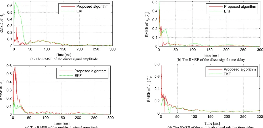
s2 is a free parameter relevant to the strength of noise and its setting can refer to [35].The proposed algorithm is compared with EKF, and the estimation results are shown in Fig. 4. In this simulation EKF setting is given as follows. The initial state of x is the true value x0 =
[
0.9, 0.4,10, 0.5]
T, the system noise covariance matrix and the initial filter covariance matrix P0 are set as Q=P0=diag(0.001*ones(1, D)), and the measurement noise
covariance matrix is set as R=diag(0.01*ones(1, D)). We can observe that the proposed algorithm has similar performance as that of EKF.
[image:9.576.61.521.311.536.2]To further inspect the performance of the proposed algorithm, the error PDFs at three observation instants are shown in Fig. 5, from which it can be observed that the shape of the error PDF, for the proposed algorithm, turns out to be narrower and sharper over the iteration process, which means the randomness of the estimation error becomes smaller. However, there is still a visible steady-state estimation error in terms of the multipath time delay. This might be caused by measurement noise. The proposed algorithm can always converge exactly to the true value when there is no noise in the system.
FIGURE 5. The error PDF for the proposed multipath estimation algorithm in single multipath environment with Gaussian noise
The constraint violation degree and the objective function of the proposed algorithm along the iterations are illustrated in Fig. 6 and Fig. 7. The same objective function is used for the proposed algorithm and the EKF. Here the same sliding window with size is used to calculate the entropy of the estimation results at each iteration. The randomness curve of the EKF estimation is also shown in Fig. 7(The result is given
[image:10.576.65.240.422.538.2]in logarithm). We can see that for the proposed algorithm the constraint violation degree decreases to zero eventually and the objective function converges to a near-zero point. The proposed algorithm outperforms EKF in respect of randomness because EKF does not take randomness into consideration during its iteration. The nonlinearity in measurement function along with the truncated error in the process of linearizing also cause a larger randomness for EKF.
FIGURE 6. The constraint violation degree profile of the filter result in
single multipath environment with Gaussian noise FIGURE 7.output error, single multipath with Gaussian noise The objective function profile for the joint measurement
For two-multipath, M = 2, D=2
(
M+ =1)
6 , 𝑁𝑁𝑝𝑝= 10𝐷𝐷 = 60, Tcon =W=60. The other parameters are set as in Table Ⅲ. In this case, Tcon is set larger than that of the single multipath case because more parameters need to be estimated for two multipath and more iterations are expected to decrease the constraint violation level to the threshold level.The estimation results are shown in Fig. 8. Similar results as that of Fig. 6 -Fig. 7 on the constraint violation and the objective function are obtained for the two multipath scenario, which are not shown here due to page limitation. In this simulation EKF setting is given as follows. The initial
state of x is the true value x0 =
[
0.9, 0.7, 0.4,10, 0.3, 0.6]
T, the system noise covariance matrix and the initial filter covariance matrix are set as Q = P0 = diag(0.001*ones(1,D)),and the measurement noise covariance matrix is set as R = diag(0.01*ones(1,D)).We can observe that the proposed algorithm achieves similar performance as EKF even when the true value is set as the initial state of EKF and the random values generated from a prior distribution are set as the initial state. In fact, the estimation result of EKF may converge to a wrong value when the initial state of EKF is set randomly from the prior distribution. In this sense, the proposed algorithm is less sensitive to the initial state.
[image:10.576.329.496.423.543.2]VOLUME XX, 2018
FIGURE 8. The estimation results in two-multipath environment with Gaussian noise
B. The non-Gaussian Noise Case
In this section, a non-Gaussian noise is constructed with the
mixture of Gaussian PDFs, i.e.
(
2)
(
2)
1 1, 1 2 2, 2
f =λN µ σ +λN µ σ , where N
(
µ σ, 2)
is a Gaussian distribution with mean μ and variance σ2.1 λ and
2
λ are the weights corresponding to the first and the second Gaussian individuals, respectively, and λ λ1+ 2=1. The parameters are set as follows: λ =1 0.9 , λ =2 0.1 ,
1 2 0
µ =µ = ,
σ
12 =10 and 2 2 100σ = . The simulation parameters are given in Table Ⅴ. Other parameters are set as the same as that in the Gaussian noise case in Section V.A.
TABLE Ⅴ
SIMULATION SETTING WITH NON-GAUSSIAN NOISE FOR SINGLE
MULTIPATH
paramete
r CRmin CRmax Fmin Fmax D Np
value 0.85 0.95 0.6 0.95 4 40 paramete
r EFmax cp Tcon Am,min Am,max γmin
value 100 5 50 0 1 -0.5 paramete
r γmax lm,min lm,max W
2
s
δ threshold
value 0.5 0 2 50 1 10-5 paramete
r λ1 λ2 µ1 µ2
2 1
σ 2
2 σ
value 0.9 0.1 0 0 10 100
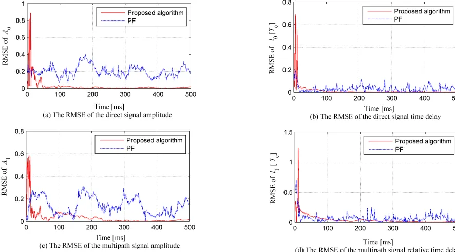
The proposed algorithm is compared with a standard PF algorithm and the results are shown in Fig. 9. In the PF algorithm, the prior density function is chosen as the importance density function. The particle number and the initial population of PF are set to be the same as in the proposed algorithm. It can be observed that the proposed algorithm clearly outperforms PF with higher estimation accuracy and smaller randomness. The error PDFs of the proposed algorithm are shown in Fig. 10, in which the error PDFs become more and more concentrated around zero mean as the iteration proceeds.
For the single path case with non-Gaussian noise, the constraint violation and the objective function of the proposed algorithm along iterations are shown in Fig. 11 and Fig. 12. Again, the same objective function is adopted to measure the randomness of estimation result for both PF and the proposed algorithm. The randomness curve of the estimation result of PF is also shown in Fig. 12 (in logarithm scale). The proposed algorithm shows less fluctuations in the objective function than that of PF. This is because although PF is more suitable for non-Gaussian noise case than for Gaussian case, it still does not take into account the randomness of its estimation result in the filter design.
For the two-multipath case with non-Gaussian noise, 6
D= , Np =10D=60 , Tcon =W =100 . The other
algorithm are shown in Fig. 13. When the same particles are used, the estimation results indicate that the proposed algorithm has higher estimation accuracy and smaller
[image:12.576.64.507.107.353.2]randomness than the PF algorithm in non-Gaussian noise environment.
[image:12.576.58.508.392.631.2]FIGURE 9. The estimation results in single multipath environment with non-Gaussian noise
VOLUME XX, 2018
FIGURE 11. The constraint violation degree profile of the filter result in
[image:13.576.80.230.74.187.2]single multipath environment with non-Gaussian noise FIGURE 12.output error, single multipath with non-Gaussian noise The objective function profile for the joint measurement
FIGURE 13. The estimation results in two-multipath environment with non-Gaussian noise
VI. CONCLUSIONS
In this paper, a new estimation algorithm is proposed for multipath estimation with Gaussian noise and non-Gaussian noise. The MEE criterion is used as the objective function. The second-order statistical information of the error as well as the prior information of the multipath parameters are taken as a set of constraints. A modified εRDE algorithm is developed to solve this constrained optimization problem to find a global solution. The simulation results demonstrate the effectiveness of the proposed algorithm for multipath estimation under both Gaussian and non-Gaussian noise environment.
[image:13.576.54.518.217.542.2]REFERENCES
[1] P. Xie and M. G. Petovello, "Measuring GNSS multipath distributions in urban canyon environments," IEEE Trans. Instrum. Meas., vol. 64, pp. 366-377, Feb. 2015.
[2] L.-T. Hsu, S.-S. Jan, P. D. Groves, and N. Kubo, "Multipath mitigation and NLOS detection using vector tracking in urban environments," GPS Solutions, vol. 19, pp. 249-262, June 2015. [3] G. Wang, K. de Jong, Q. Zhao, Z. Hu, and J. Guo, "Multipath analysis of code measurements for BeiDou geostationary satellites," GPS solutions, vol. 19, pp. 129-139, Apr.2015. [4] J. M. Tranquilla, J. Carr, and H. M. Al-Rizzo, "Analysis of a
choke ring groundplane for multipath control in global positioning system (GPS) applications," IEEE Trans. Antennas Propag., vol. 42, pp. 905-911, July 1994.
[5] J. Ray, M. Cannon, and P. Fenton, "GPS code and carrier multipath mitigation using a multiantenna system," IEEE Trans. Aerosp. Electron. Syst., vol. 37, pp. 183-195, Jan. 2001. [6] R. Nee, "The multipath estimating delay lock loop," in Proc. 2nd
IEEE ISSSTA, Las Vegas, NV, USA , 1992, pp. 39-42. [7] V. A. Dierendonck, P. Fenton, and T. Ford, "Theory and
performance of narrow correlator spacing in a GPS receiver," Navigation, vol. 39, pp. 265-283, Sept. 1992.
[8] L. Garin, F. van Diggelen, and J.-M. Rousseau, "Strobe and edge correlator multipath mitigation for code," in ION GPS-96, 1996, pp. 657-664.
[9] X. Chen, F. Dovis, S. Peng, and Y. Morton, "Comparative studies of GPS multipath mitigation methods performance," IEEE Trans. Aerosp. Electron. Syst., vol. 49, pp. 1555-1568, July 2013.
[10] T. Takahama and S. Sakai, "Efficient constrained optimization by the ε constrained rank-based differential evolution," in Evolutionary Computation (CEC), 2012 IEEE Congress on, 2012, pp. 1-8.
[11] W. Nam and S. H. Kong, "Least-squares-based iterative multipath super-resolution technique," IEEE Trans. Signal Process., vol. 61, pp. 519-529, Feb 2013.
[12] J. Y. Kim, "PN code tracking loop with extended Kalman filter for a direct-sequence spread-spectrum system," in Industrial Electronics Society, 2004. IECON 2004. 30th Annual Conference of IEEE, Busan, South Korea, 2004, pp. 2637-2640.
[13] D. Erdogmus and J. C. Principe, "Comparison of entropy and mean square error criteria in adaptive system training using higher order statistics," in Proc. ICA, 2000, pp. 75-80. [14] R. B. Wu, W. Y. Wang, D. Lu, et al, "Multipath interference
suppression" in Adaptive interference mitigation in GNSS, Beijing, China: Science Press, chapter 5, 2018, pp. 201-233. [15] M. Ren, J. Zhang, F. Fang, G. Hou, and J. Xu, "Improved
minimum entropy filtering for continuous nonlinear non-Gaussian systems using a generalized density evolution equation," Entropy, vol. 15, pp. 2510-2523, July 2013. [16] M. Ren, T. Cheng, J. Chen, X. Xu, and L. Cheng, "Single neuron
stochastic predictive PID control algorithm for nonlinear and non-Gaussian systems using the survival information potential criterion," Entropy, vol. 18, p. 218, 2016.
[17] P. M. Djuric, J. H. Kotecha, J. Zhang, Y. Huang, T. Ghirmai, M. F. Bugallo, et al., "Particle filtering," IEEE signal processing magazine, vol. 20, pp. 19-38, 2003.
[18] L. Cheng, M. Ren, G. Xie, and J. Chen, "Multipath estimation using kernel minimum error entropy filter," in Control (CONTROL), 2016 UKACC 11th Int. Conf. on, 2016, pp. 1-5. [19] H. Wang, "Robust control of the output probability density
functions for multivariable stochastic systems with guaranteed stability," IEEE Trans. Autom. Control, vol. 44, pp. 2103-2107, Nov. 1999.
[20] H. Wang and H. Yue, "A rational spline model approximation and control of output probability density functions for dynamic stochastic systems," Transactions of the Institute of Measurement and Control, vol. 25, pp. 93-105, 2003.
[21] B. Chen, Y. Zhu, J. Hu, and J. C. Principe, System parameter identification: information criteria and algorithms: Newnes, 2013.
[22] L. Guo and H. Wang, "Minimum entropy filtering for multivariate stochastic systems with non-Gaussian noises," IEEE Trans. Autom. Control, vol. 51, pp. 695-700, Apr 2006. [23] J. W. Xu, D. Erdogmus, and J. C. Principe, "Minimum error
entropy Luenberger observer," in American Control Conference, 2005. Proceedings of the 2005, 2005, pp. 1923-1928.
[24] J. Zhang, L. Cai, and H. Wang, "Minimum entropy filtering for networked control systems via information theoretic learning approach," in Modelling, Identification and Control (ICMIC), The 2010 International Conference on, 2010, pp. 774-778. [25] M. Ren, J. Zhang, and H. Wang, "Minimized tracking error
randomness control for nonlinear multivariate and non-gaussian systems using the generalized density evolution equation," IEEE Trans. Autom. Control, vol. 59, pp. 2486-2490, Sept. 2014. [26] L. Cheng, M. F. Ren, and G. Xie, "Multipath estimation based
on centered error entropy criterion for non-Gaussian noise," IEEE Access,vol.4,pp. 9978-9986, Dec.2016.
[27] M. F. Ren, "Research on control and filtering for non-Gaussian systems," Ph. D. dissertation, North China Electric Power Univ., Beijing 2014.
[28] J. S. Vera, "Efficient multipath mitigation in navigation systems," in Ph. D. dissertation, Universitat Politecnica de Catalunya, 2004.
[29] L. Cheng, J. Chen, and G. Xie, "Model and simulation of multipath error in DLL for GPS receiver," Chinese Journal of Electronics, vol. 23, pp. 508-515, 2014.
[30] P. Closas, C. Fernandez-Prades, and J. A. Fernandez-Rubio, "A Bayesian approach to multipath mitigation in GNSS receivers," IEEE J. Sel. Topics Signal Process.,vol. 3, pp. 695-706, July 2009.
[31] Y. Z. Wang, X. Chen, P. L. Liu, et al, " Study on multipath model of BDS/GPS signal in urban canyon " in CSNC 2017, 2017, vol 2, pp. 95-105.
[32] D. Xu and D. Erdogmuns, "Renyi’s entropy, divergence and their nonparametric estimators," in Information Theoretic Learning, ed: Springer, 2010, pp. 47-102.
[33] G. Y. Chen, M. Gan, C. L. Philip Chen, et al, "A two-stage estimation algorithm based on variable projection method for GPS positioning," IEEE Trans. Instrum. Meas., to be published. DOI: 10.1109/TIM.2018.2826798.
[34] M. Lentmaier, B. Krach, and P. Robertson, "Bayesian time delay estimation of GNSS signals in dynamic multipath environments," Int. J. Navigation Observation, vol. 2008, Mar. 2008.
[35] Y. Liu, H. Wang, and C. Hou, "UKF based nonlinear filtering using minimum entropy criterion," IEEE Trans. Signal Process., vol. 61, pp. 4988-4999, Oct. 2013.
Lan Cheng (M’16) received the M.S. degree in
Control Theory and Control Engineering from the Taiyuan University of Technology, Taiyuan, Shanxi, China, in 2008. She received the PhD. degree in Control Science and Engineering from Beijing Institute of Technology, Beijing, China, in 2012.
Hong Yue (M’99, S’04) received the B.Eng. and the M.Sc. degrees in process control engineering from Beijing University of Chemical Technology, Beijing, China in 1990 and 1993, respectively, and the Ph.D. degree in control theory and applications from East China University of Science and Technology, Shanghai, China in 1996. She is a senior lecturer at the Department of Electronic and Electrical Engineering, University of Strathclyde. Her research interests are in systems and control with a focus on modelling, control and optimization of complex systems.
Yan J. Xing received theBachelor’s degree in
Automation from Tianjin University of Science and Technology, Tianjin, in 2015 and the M. S. degree in Control Science and Control Engineering from Taiyuan University of Technology, Taiyuan, China, in 2018. She is currently an engineer in China Unicom Ltd, Taiyuan, Shanxi, China. Her major research interests include multipath mitigation, intelligent control theory and application.
Mi F. Ren (M’12)received the M.S. degree in