Twin Peaks

City, University of London Institutional Repository

Citation

: Defever, F. and Riaño, A. (2017). Twin Peaks (17/02). London, UK: Department

of Economics, City, University of London.

This is the published version of the paper.

This version of the publication may differ from the final published

version.

Permanent repository link:

Link to published version

: 17/02

Copyright and reuse:

City Research Online aims to make research

outputs of City, University of London available to a wider audience.

Copyright and Moral Rights remain with the author(s) and/or copyright

holders. URLs from City Research Online may be freely distributed and

linked to.

Department of Economics

Twin Peaks

Fabrice Defever

City, University of London

Alejandro Riaño

University of Nottingham

Department of Economics

Discussion Paper Series

No. 17/02

Twin Peaks

Fabrice Defever†, Alejandro Ria˜no‡

October 20, 2017

Abstract

Received wisdom suggests that most exporters sell the majority of their output domestically. In this paper, however, we show that the distribution of export intensity not only varies substan-tially across countries, but in a large number of cases is also bimodal, displaying what we refer to as twin peaks. We reconcile this new stylized fact with an otherwise standard, two-country model of trade in which firms are heterogeneous in terms of the demand they face in each market. We show that when firm-destination-specific revenue shifters are distributed lognormal, gamma, or Fr´echet with sufficiently high dispersion, the distribution of export intensity has two modes in the boundaries of the support and their height is determined by a country’s size relative to the rest of the world. We estimate the deep parameters characterizing the distribution of export intensity. Our results show that when the conditions for the existence of twin peaks are met, differences in relative market size can explain most of the observed variation in the distribution of export intensity across the world.

Keywords: Exports; Export Intensity Distribution; Bimodality; Firm Heterogeneity. JEL classification: F12, F14, C12, O50.

∗

We thank Peter Egger, Julian di Giovanni, Keith Head, Chris Jones, Emanuel Ornelas, Veronica Rappoport, Dani Rodrik, and seminar participants at Universitat Barcelona, ETH Zurich, LSE/CEP, Universidad del Rosario, the 2015 EIIT conference at Purdue University, the 2016 Royal Economic Society Meetings, the 2016 conference in Industrial Organization and Spatial Economics, St. Petersburg and the 2017 SED Annual Meetings for their helpful comments. We would like to thank Facundo Albornoz-Crespo, Salamat Ali, Roberto Alvarez, Paulo Bastos, Carlos Casacuberta, Banu Demir, Ha Doan, Robert Elliott, Mulalo Mamburu, Sourafel Girma, Kozo Kiyota, Bal´asz Murak¨ozy and Steven Poelhekke for sharing their data or export intensity moments with us. All remaining errors are our own.

†

City, University of London; GEP; CESifo and CEP/[email protected] ‡

1

Introduction

Received wisdom suggests that most exporters sell the majority of their output domestically

(Bernard et al., 2003; Brooks, 2006; Arkolakis, 2010; Eaton et al., 2011). This is considered one of the key empirical regularities that characterize the behavior of firms engaged in international

trade, summarized in the reviews byBernard et al. (2007) andMelitz and Redding(2014).1 In this paper we challenge this notion. Using harmonized cross-country firm-level data from the World Bank Enterprise Surveys (WBES), we show that the distribution of export intensity —

the share of sales accounted for by exports conditional on exporting— varies tremendously across

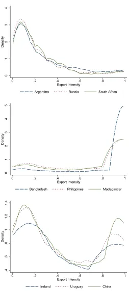
countries.2 This is vividly illustrated in Figure 1. Countries like Argentina, Russia and South Africa exhibit the same pattern identified in previous studies; firms with export intensity below

0.2 constitute more than half of exporters, while firms with an export intensity above 0.8 account for less than 10% of exporters. In Bangladesh, Madagascar and the Philippines, we observe the

opposite pattern —the average share of exporters with intensity below 0.2 and above 0.8 are,

respectively, 11% and 75%. A large number of countries (China, Ireland and Uruguay, to name a few) also display ‘twin peaks’ —a high concentration of firms on both ends of the distribution. In

fact, we find that unimodality is rejected for two-thirds of the countries in our data. To the best

of our knowledge, we are the first in identifying this novel stylized fact.

The workhorse models of international trade in which firms only differ in their productivity,

such asMelitz(2003), are at odds with the wide range of patterns presented in Figure1. In a

two-country model with CES preferences, all exporters sell the same share of their revenues abroad; i.e. the distribution of export intensity is degenerate. When there are more than two countries, more

productive firms have a higher export intensity than less productive ones, because the former serve

more markets than the latter. If the model is to be consistent with the well-established fact that a small number of large firms coexist with a large number of small firms (see Simon and Bonini,

1958;Axtell,2001), then it would not be able to generate right-skewed nor bimodal export intensity

distributions.3

We show, however, that with one single adjustment, the standard two-country model of trade

with CES preferences can reproduce the wide variety of shapes depicted in Figure1very successfully.

Namely, we require large idiosyncratic differences in the demand that firms face domestically and abroad. When the firm-destination-specific revenue shifters that generate these differences are

distributed lognormal, gamma or Fr´echet —three of the distributions most frequently used to

model firm heterogeneity— with sufficiently high dispersion, then the probability density function of export intensity is bimodal. The modes of the distribution are located near 0 and 1 and their

1

The other two stylized facts identified by the literature are that only a minority of firms engage in exporting and that exporters perform better than domestic firms. These two results have been verified for almost every country in the world.

2_{In Section2we show that these patterns also arise when we use more representative data from national}

manu-facturing surveys. 3

Figure 1: Export Intensity Distribution Across Countries: Selected Examples

0

1

2

3

4

Density

0 .2 .4 .6 .8 1

Export Intensity

Argentina Russia South Africa

0

1

2

3

4

5

Density

0 .2 .4 .6 .8 1

Export Intensity

Bangladesh Philippines Madagascar

.4

.6

.8

1

1.2

1.4

Density

0 .2 .4 .6 .8 1

Export Intensity

Ireland Uruguay China

‘height’ is determined by a country’s relative market size with respect to the rest of the world. Thus,

the interaction between large heterogeneity in firms’ performance across markets and differences in relative market size can explain the observed variation in the distribution of export intensity across

countries.

Using firm-level data for 72 countries drawn from several waves of the WBES over the period 2002-2016, we estimate the deep parameters that characterize the distribution of export intensity.

These are the shape parameter of the distribution of firm-destination-specific revenue shifters and a

country’s relative market size with respect to the rest of the world. We tease out the latter directly from the data by exploiting the fact that for all the underlying distributions of revenue shifters

we consider, there is a one-to-one relationship between relative market size and the median export

intensity which is independent of the shape parameter. Conditional on this inferred measure of relative market size, we estimate the shape parameter by maximum likelihood. The identification of

the parameters is very transparent: if the conditions for twin peaks are satisfied, greater dispersion

of revenue shifters (which is determined by the shape parameter) increases the distribution’s mass in the extremes of the support. For a given level of dispersion, changes in market size shift mass

from one extreme of the support to other. Conversely, if the dispersion of revenue shifters is not

sufficiently high, then the distribution of export intensity would be unimodal and its mass would be tightly concentrated around its median in the interior of the support.

The results provide strong support for the existence of twin peaks. When we estimate country-specific scale and shape parameters, the conditions for bimodality are satisfied in all but a handful

of cases. We then estimate a model in which all cross-country variation in the distribution of

export intensity is accounted for by differences in relative market size, since firms in every country draw revenue shifters from a distribution with the same shape parameter. Our results are striking.

Conditional on relative market size, we are are able to fit the distribution of export intensity

across the wide range of countries in our data with only one shape parameter. This provides the main takeaway message from the paper: conditional on firm-destination-specific factors exhibiting

sufficiently high dispersion, differences in relative market size explain most of the observed variation

in the distribution of export intensity across the world.

We carry out a thorough robustness analysis of our main result. More specifically, we explore

the possibility that the bimodality of the export intensity distribution is the result of a composition

effect —i.e. if most exporters were low-intensity ones, but specific subsets were particularly inclined to export most of their output. We find that the dispersion of firm-destination-specific revenue

shifters remains sufficiently high to generate bimodality when we exclude multinational affiliates,

firms engaged in processing activities, and even firms exporting all their output. Similarly, excluding countries that provide subsidies conditioned on firms’ export performance or splitting our sample

according to countries’ level of development leaves our results intact. We also show that bimodality

is not a product of a country’s sectoral composition of exports. In our last robustness exercise, we work directly with domestic and export sales instead of export intensity data. Doing so allows us

out a variance decomposition of sales in each market. The latter reveals that —consistent with the

empirical literature relying on customs data (Kee and Krishna, 2008; Munch and Nguyen, 2014;

Lawless and Whelan,2014, e.g.)— firm-destination-specific factors account for a large share of the

variation in firms’ sales in a given destination.

Understanding export intensity is important on its own right. In the paper we show that the existence of twin peaks affects the response of the export intensity distribution to reductions in

trade costs as well as the sales diversification benefits of exporting. Characterizing accurately the

distribution of export intensity in an undistorted economy is also a key input to infer the magnitude of distortions that affect firms’ access to foreign markets, following the approach pioneered byHsieh

and Klenow(2009). This strategy has been used byBrooks and Wang(2016) to quantify the effect

of idiosyncratic trade taxes and preferential access to foreign exchange, and byDefever and Ria˜no

(2017a) to evaluate the welfare cost of incentives subject to export performance requirements.

Alessandria and Avila (2017) rely on changes in the distribution of export intensity over time to

discipline a model that quantifies the contribution of technology and trade policy in Colombia’s process of trade opening. Export intensity has also been show to be strongly correlated with a wide

variety of outcomes such as female employment (Ozler, 2000), lobbying activity on trade policy

(Osgood et al., 2017) and financial constraints (Egger and Erhardt, 2014). Kohn et al. (2017) show that the response of aggregate exports to large devaluations in emerging markets, where

exporters often borrow in foreign currency, is crucially shaped by the distribution of export intensity.

Alfaro et al.(2017) show that differences in average export intensity explain why East Asian firms’

productivity and R&D investment are more responsive to real exchange rate depreciations than

their counterparts in Europe and Latin America.

Our paper is related to several strands in the literature. First, we add to the recent work that

investigates the implications of using different probability distributions to model firm heterogeneity

in international trade models (Head et al.,2014;Mr´azov´a et al.,2015;Nigai,2017). While most of this literature focuses on productivity, we highlight the importance of the idiosyncratic interaction

between individual firms and markets. The importance of firm-destination factors in explaining

export sales variation has been identified byEaton et al.(2011),Crozet et al.(2012) andFernandes et al. (2015). We show that this feature of the data can also explain the variation of the export

intensity distribution across countries. Our work is also related toLu(2010) andDefever and Ria˜no

(2017a), who first documented the fact that the export intensity distribution in China is markedly bimodal. Our work shows that this pattern is not specific to China, and is, in fact, quite common

across the world.

The rest of the paper is organized as follows. Section 2presents the data used in our analysis, documents the prevalence of bimodality in the distribution of export intensity across countries and

provides a comparison with more representative, national firm-level surveys for a selected subset of

countries. Section 3 presents our theoretical framework. We show the conditions under which the distribution of export intensity is bimodal and discuss implications of the existence of twin peaks.

Section5reports the results of an extensive battery of robustness checks to our main specification.

Section6 concludes.

2

Data

Our data comes from several waves of the World Bank Enterprise Surveys (WBES) spanning the

period 2002-2016. These surveys are carried out by the World Bank’s Enterprise Analysis Unit (usually every 3-4 years) using a uniform methodology and questionnaire, and are intended to be

representative of a country’s non-agricultural private economy.4 The unit of observation in the surveys is the establishment, i.e. a physical location where business is carried out or industrial operations take place, which should have its own management and control over its own workforce.

Since the vast majority of establishments surveyed report to be single-establishment firms, hereafter

we refer to them as ‘firms’. We use the data for the manufacturing sector only (i.e. firms that belong to ISIC Rev. 3.1 sectors 15-37).

The WBES provides information on firms’ main sector of operation, total sales, export intensity, ownership status (whether the firm is domestic or foreign-owned), labor productivity and the share

of material inputs accounted for by imports. The main variable of interest is export intensity —the

share of sales that a firm exported, both directly or indirectly through an intermediary, in a fiscal year— and is therefore defined on the intervalp0,1s.5

Our sample consists of 72 developing and transition countries (with the exception of Ireland

and Sweden), for which we observe at least 97 exporting firms when we pool the data across all available survey waves. Table 1 lists the countries in our sample and provides information on the

number of exporters and survey waves. The number of exporters per country ranges from 97 in

Ireland to 2,112 in India, accounting, on average, for 40% of firms surveyed in a country. In terms of geographic coverage, the countries in our data are evenly distributed across Eastern Europe,

Latin America and the Caribbean, Asia and the Middle East and Africa; Ireland and Sweden are

the only two countries in our sample from Western Europe.

Table 1 also indicates whether a country provides incentives that are directly conditioned on

firms’ export intensity.6 Defever and Ria˜no (2017a) investigate the effects that these subsidies subject to export share requirements (ESR) have on the intensity of competition and welfare in the context of China. We rely on information from the “Performance Requirements and Incentives” and

“Foreign Trade Zones/Free Trade Zones” sections of the Investment Climate Statements produced

by the U.S. State Department to identify countries offering these incentives. Table 1 reveals that

4_{More specifically, the survey targets formal (registered) firms with more than 5 employees that are not 100%}

state-owned. 5

Since the survey asks firms directly about the percentage of their sales exported, the response is bounded at 100%, and therefore does not capture ‘carry along’ trade —a phenomenon first identified byBernard et al.(2012)— in which firms export goods that they do not produce.

6_{Examples include direct cash transfers, tax holidays and deductions, and the provision of utilities at below-market}

subsidies subject to ESR are pervasive in developing countries, with half of the countries in our

data employing them.

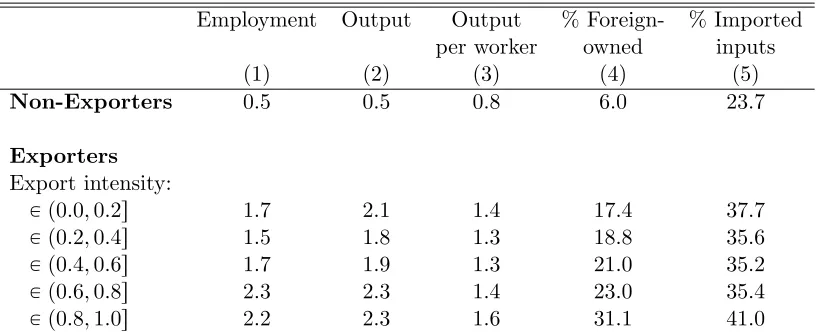
Table 2: Firm Characteristics by Export Status and Export Intensity

Employment Output Output % Foreign- % Imported

per worker owned inputs

(1) (2) (3) (4) (5)

Non-Exporters 0.5 0.5 0.8 6.0 23.7

Exporters Export intensity:

P p0.0,0.2s 1.7 2.1 1.4 17.4 37.7

P p0.2,0.4s 1.5 1.8 1.3 18.8 35.6

P p0.4,0.6s 1.7 1.9 1.3 21.0 35.2

P p0.6,0.8s 2.3 2.3 1.4 23.0 35.4

P p0.8,1.0s 2.2 2.3 1.6 31.1 41.0

Columns (1)-(3) report the average across countries of the relative size and labor productivity of ex-porters and domestic firms relative to the mean value of each variable calculated in each country-survey year cell. Thus, for instance, domestic firms across all countries in our sample are 50% smaller (in terms of employment) than the average firm, while exporters with an export intensity lower than 20% are 70% larger than the average firm. Column (4) reports the percentage of foreign-owned firms (firms with a share of foreign equity at least 10% or greater) and column (5) presents the percentage of imported inputs in total intermediate inputs in each export intensity bin.

Table2 provides a first pass at the data comparing exporters (along the distribution of export intensity) with domestic firms across various performance measures. Columns (1)-(3) provide

in-formation on firm size and productivity relative to the average value of the respective statistic in

each country-survey year pair. Columns (4) and (5) report the percentage of foreign-owned firms and the use of imported inputs. Table 2 reveals that —consistent with the evidence summarized

by Bernard et al. (2007) and Melitz and Redding(2014)— exporters are larger (both in terms of

employment and output) and more productive than domestic firms in our sample. Looking across the export intensity distribution, we find that although there is a positive correlation between firm

size and export intensity, there is not a clear relationship between labor productivity and export

intensity.7 Columns (4) and (5) show that exporters — and high-intensity ones in particular— are more likely to be foreign-owned (Antr`as and Yeaple,2014) and to use imported intermediate inputs

more intensively than domestic firms (Amiti and Konings,2007).

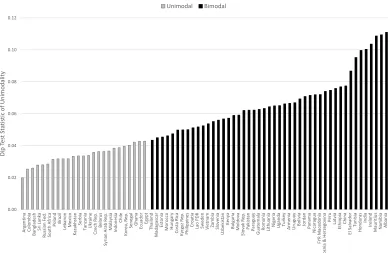
While Figure 1 provides suggestive evidence about export intensity distributions exhibiting twin peaks, we now carry out a systematic statistical test of unimodality in our data, using the

so-called dip statistic proposed by Hartigan and Hartigan (1985). This test measures departures

from unimodality in the empirical cumulative distribution function (cdf) by relying on the fact that

7

Figure 2: Dip Test of Unimodality of Export Intensity 0.00 0.02 0.04 0.06 0.08 0.10 0.12 A rg en ti n a Co lo mb ia Ba n gl ad es h Sr i L an ka R u ss ian F ed . So u th A fri ca Po la n d Braz il Le b an o n Me xi co Kaz ak h stan Se rb ia Ta n za n ia Uk rai n e Cz ec h R ep . Bel aru s Syr ian A rab R ep . Mal ays ia In d o n es ia Ch ile Ko re a, R e p . Se n e gal G h an a Ec u ad o r Eg yp t Th ail an d Mad ag as car Es to n ia Mo ro cc o H u n gary Co sta R ic a Kyrg yz R ep . Phi lip p in e s Cro ati a La o P DR Sw ed en V ie tn am Zamb ia Sl o ve n ia Uzbe ki stan Ke n ya Bul gari a Mo ld o va Sl o vak R ep . Pa ki stan Pa rag u ay G u ate mala R o man ia Li th u an ia N ig eri a Ug an d a Tu rk e y A rme n ia Ur u gu ay Bo livia Jo rd an Pa n ama N ic arag u a FY R Mac e d o n ia Bo sn

ia & H

er ze go vin a Per u La tv ia Eth io p ia Ch in a El S alvad o r Tu n is ia H o n d u ras In d ia Ire lan d Mau ri ti u s N amib ia A lb an ia D ip T es t St at is tic of Un imo d alit y Unimodal Bimodal

The figure reports the value of the Hartigan and Hartigan(1985) dip test statistic of unimodality. Countries are identified as having having a unimodal export intensity distribution if their dip statistic does not reject the null hypothesis of unimodality at the 1% confidence level; otherwise, they are identified as bimodal. The reported value of the dip statistic is calculated as the mean across 1,000 bootstrapped samples of 200 exporters drawn for each country. The algorithm used to calculate the dip test statistic is adjusted to take into account the discreteness of the export intensity data.

a unimodal distribution has a unique inflection point.8 As Henderson et al. (2008) note, the dip measures the amount of ‘stretching’ needed to render the empirical cdf of a multi-modal distribution unimodal. Thus, a higher value for the dip leads to a rejection of the null hypothesis of unimodality.

Hartigan and Hartigan (1985) choose the uniform distribution as the null distribution because its

dip is the largest among all unimodal distributions. The dip test has been widely used in economics to, among other things, identify convergence clusters in the distribution of GDP per capita, total

factor productivity and other indicators of economic growth (Henderson et al.,2008), characterize

the degree of price stickiness (Cavallo and Rigobon,2011) and to assess the identification of hazard function estimates (Heckman and Singer,1984).

Figure2presents the dip statistic for all countries in our sample. We identify the distribution of

export intensity in a country as unimodal if the null hypothesis of the dip statistic is not rejected at the 1% significance level at least; otherwise, we consider it to be bimodal.9 Based on this criterion, we find that the distribution of export intensity is bimodal in 47 out of 72 countries. As we noted

in the introduction, this result stands in sharp contrast with previous work suggesting that this

8_{More precisely, the cdf is convex on the interval}

p´8, xmqand concave betweenpxm,`8q, wherexmdenotes the

unique mode of the distribution.

9_{Although the dip test only tells us whether a distribution is unimodal or not, visual inspection of kernel densities}

distribution was generally unimodal, with a majority of exporters selling a small share of their

output abroad.

There are two important points that need to be made regarding the calculation of our dip test.

Firstly, since the WBES survey questionnaire asks directly ‘what percentage of the establishment’s

sales were exported’, the response to this question tends to cluster in figures that are multiples of 5%. Therefore, we adjust the dip statistic to take into account the discreteness of the data, since

not doing so would lead to over-rejecting the null hypothesis of unimodality. Secondly, since the

number of exporters varies substantially across countries, the dip statistic reported in Figure 2 is calculated as the mean across 1,000 bootstrapped samples of 200 exporters in each country, which

allows us to directly compare the dip across countries.

Is the high prevalence of twin peaks in the distribution of export intensity a figment of the WBES data? Asker et al. (2014), for instance, note that the stratification procedure across sectors, size

categories and geographic locations used in the construction of the WBES leads to an oversampling

of larger firms relative to a random sample of all firms in the economy. Although it is not clear that this would necessarily increase the likelihood of observing bimodal export intensity distributions,

it is crucial for our purposes to show that twin peaks also appear in more representative datasets.

To this end, we asked fellow researchers to calculate for us the share of exporters across export intensity bins using well-known firm-level manufacturing surveys for a sub-sample of 13 countries

in our data.10 The countries that we consider include 5 that we classify as unimodal based on the dip statistic (Argentina, Chile, Colombia, Indonesia and South Africa) and 8 bimodal (China,

Hungary, India, Ireland, Pakistan, Thailand, Uruguay and Vietnam). Most surveys used in our

analysis include all manufacturing firms with more than 10 to 20 employees, although the data for China and Ireland is based on a survey of larger firms. It is also important to note that the

distribution of export intensity based on manufacturing surveys is calculated with data for a single

year, whereas —as we have noted above— the data we use pools exporters from all survey waves available for a given country in the WBES.

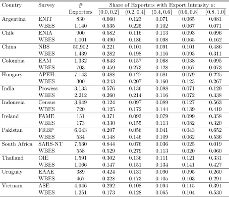
Table 3 presents the comparison between the distribution of export intensity based on

man-ufacturing surveys and the one based on WBES data. The key message is that the WBES data provides an accurate picture of the distribution export intensity. Both data sources yield

simi-lar results with regards to the existence or not of twin peaks —even in the cases in which there

are significant differences in the share of exporters in individual bins (e.g. in Hungary and India). Crucially, note that in all countries but one, the share of exporters with export intensity in the

middle bins (where export intensity is between 0.2 and 0.8) is higher in the WBES than in the

more representative data. Thus, if anything, it seems that we are underestimating the prevalence of twin peaks by relying on the WBES data.

10

The choice of these countries was driven by data availability. The manufacturing survey data that we rely upon for the comparison has been used in a large number of prominent papers in international trade, including —but not limited to— Bustos (2011) (Argentina), Alvarez and L´opez (2005) (Chile), Feenstra and Hanson (2005) (China),

Roberts and Tybout (1997) (Colombia), B´ek´es and Murak¨ozy (2012) (Hungary), Goldberg et al. (2010) (India),

Javorcik and Poelhekke(2017) (Indonesia),Ali et al.(2017) (Pakistan),Mamburu(2017) (South Africa),Cole et al.

Table 3: Comparison of Export Intensity Distributions —WBES vs Other Surveys

Country Survey # Share of Exporters with Export Intensity P:

Exporters p0.0,0.2s p0.2,0.4s p0.4,0.6s p0.6,0.8s p0.8,1.0s

Argentina ENIT 830 0.660 0.123 0.071 0.065 0.081

WBES 1,140 0.535 0.225 0.102 0.067 0.071

Chile ENIA 900 0.582 0.116 0.113 0.093 0.096

WBES 1,001 0.490 0.186 0.098 0.065 0.162

China NBS 50,902 0.221 0.101 0.091 0.101 0.486

WBES 1,439 0.282 0.198 0.116 0.093 0.311

Colombia EAM 1,332 0.643 0.157 0.068 0.038 0.095

WBES 703 0.459 0.273 0.128 0.067 0.073

Hungary APEH 7,143 0.488 0.127 0.081 0.079 0.225

WBES 300 0.243 0.207 0.160 0.123 0.267

India Prowess 3,133 0.576 0.136 0.088 0.071 0.129

WBES 2,212 0.260 0.214 0.116 0.072 0.338

Indonesia Census 3,949 0.124 0.097 0.089 0.127 0.563

WBES 720 0.125 0.172 0.144 0.139 0.419

Ireland FAME 151 0.371 0.093 0.079 0.099 0.358

WBES 173 0.330 0.155 0.113 0.082 0.320

Pakistan FRBP 6,043 0.207 0.056 0.041 0.043 0.652

WBES 534 0.148 0.146 0.109 0.062 0.536

South Africa SARS-NT 7,530 0.844 0.076 0.036 0.025 0.019

WBES 558 0.529 0.279 0.113 0.020 0.060

Thailand OIE 1,591 0.302 0.136 0.111 0.121 0.331

WBES 1,066 0.147 0.151 0.134 0.141 0.427

Uruguay EAAE 389 0.424 0.131 0.090 0.095 0.260

WBES 467 0.328 0.173 0.105 0.103 0.291

Vietnam ASE 4,946 0.292 0.108 0.094 0.115 0.391

WBES 1,251 0.173 0.128 0.065 0.104 0.530

3

Theoretical Framework

Consider a monopolistically-competitive industry in which each firm produces a unique,

differen-tiated good indexed by ω (which will also denote a firm’s identity hereafter). Firms can sell their output domestically (d), or export it to the rest of the world (x). Firm ω’s sales in destination market iP td, xu,ripωq, are given by:

ripωq “Ai¨zipωq ¨pipωq1´σ, (1)

where pipωq is the price charged by firm ω in market i, σ ą 1 is the elasticity of demand, Ai is

a measure of market i’s size —which is common to all firms selling there— and zipωq is a firm-destination-specific revenue shifter.11 _{Our choice for the underlying distribution of revenue shifters}

(lognormal, gamma or Fr´echet) is driven both by their wide usage to model economic heterogeneity

and, as noted below, the need for a closed-form expression for the pdf of the ratio of revenue shifters.12

Recent work has shown that idiosyncratic, destination-specific factors, such as cross-country

differences in tastes, the extent of a firm’s network of customers or its participation in global value chains are important drivers of firms’ export decisions (Eaton et al.,2011;Demidova et al., 2012;

Crozet et al.,2012). In fact, empirical evidence for Bangladeshi, Danish, French and Irish exporters

has consistently found that firm-destination fixed effects account for a similar share of the variation in export sales as firm-specific factors such as productivity (see respectively, Kee and Krishna

(2008),Munch and Nguyen (2014), Eaton et al.(2011), andLawless and Whelan (2014)).

As is standard in international trade models with heterogenous firms, producers pay a sunk cost fe to draw their idiosyncratic productivity, ϕ, from a distribution with probability density

function (pdf), gpϕq.13 Firms draw their idiosyncratic revenue shifter in market i, zipωq, from a distribution with pdf fpziq. We assume that the distribution fp¨q is the same in both markets, although its parameters can, in some cases, differ across destinations; furthermore, revenue shifters

and productivity are assumed to be orthogonal with respect to each other. Firms incur a fixed cost

fd to set up a plant and produce their respective good using a linear technology, with labor being

the only input. Thus, the marginal cost of production for a firm of productivity ϕ, is w{ϕ, where

11

The revenue function (1) obtains when there is a representative consumer in each country with CES preferences of

the form:U“

” ř

iPtd,xu

´ ş

ωPΩirzipωq

1

σ´1_q

ipωqs

σ´1

σ _dω

¯ı_σ´σ₁

, whereqipωqdenotes the quantity of goodωfrom country iconsumed, and Ωiis the set of varieties produced in marketiavailable to consume. Under this interpretation, market i’s size is given byAi”RiPiσ´1, whereRi denotes countryi’s aggregate expenditure andPiis the ideal price index

prevailing in the same country. 12

The lognormal distribution has recently become a popular alternative to model the distribution of firm-level productivity in international trade (see e.g. Head et al., 2014; Mr´azov´a et al., 2015; Nigai, 2017); Hanson et al.

(2016) find that the distribution of export capabilities at the industry level is also well approximated by a lognormal distribution. Both Eaton et al.(2011) and Fernandes et al.(2015) use the lognormal distribution to model firm-destination-specific revenue shifters in models with more than two destination markets. Luttmer (2007) uses the gamma distribution to model the size distribution of firms, whileEaton and Kortum(2002) is the seminal reference on the use of the Fr´echet distribution to model cross-country differences in productivity.

13

w is the wage prevailing in the domestic market. A firm that chooses to export needs to incur an additional fixed cost,fx, and an iceberg transport cost,τ ě1.

Remark. We assume that firms choose whether to operate or not and what markets to serve after

observing their productivity, butbefore knowing the realization of revenue shifters.

We get a lot of mileage from this assumption.14 As will become clearer below, it allow us to derive the pdf of export intensity only requiring knowledge of the distribution of the ratio of relative revenue shifters. Moreover, we will also show that when revenue shifters are distributed

lognormal, gamma or Fr´echet, we can back out the relative market sizesd{sxdirectly from the data

without having to solve the full model in general equilibrium. If, on the other hand, firms made the decision to export after observing both their productivity and revenue shifters, then the distribution

of export intensity would depend on the joint distribution of these variables and the truncation

caused by the fixed cost of exporting;15 Defever and Ria˜no (2017a) calibrate the distribution of export intensity in the latter type of model.

A firm that is productive enough to export,16 sets pricespdpωq “ _σσ_´1w_ϕ and pxpωq “τ pdpωqat home and abroad respectively (since revenue shifters are multiplicative, they do not affect prices). Sales in market iP td, xu are given by:

ripωq “Φpωq ¨si¨zipωq, (2)

where sd ” `_σ´1

σ ˘σ´1

w1´σ_A

d, sx ” `_σ´1

σ ˘σ´1

w1´σ_τ1´σ_A

x, and Φpωq ” ϕσ´1. Thus, sales in a

given destinationiare composed of three terms: siencompasses all variables that are common across

all firms selling ini(i.e. marketi’s size, home’s wage, transport costs), Φpωq (productivity), varies across firms but is the same across destinations, and zipωq represents the factors that determine the appeal of firm ω’s product specifically in market i.

Define an exporting firm’s export intensity as the share of total sales accounted for by exports. LetEpωqbe the random variable denoting the export intensity of firmω, while lowercaseedenotes a realization of this random variable. Thus, the export intensity for firm ω is given by:

Epωq ” rxpωq

rdpωq `rxpωq “

sxzxpωq

sdzdpωq `sxzxpωq

“ Zxpωq

Zdpωq `Zxpωq. (3)

Since firms can only sell their output in two destinations, and charge the same constant markup in

both, it follows that export intensity is independent of productivity. Thus, in the absence of

firm-14_{This timing assumption has also been used byCherkashin et al.(2015); it is consistent with the fact that while}

firm-level productivity strongly predicts export entry, it explains much less of the variation in sales across destinations conditional on entry (Eaton et al.,2011).

15

Under this assumption the decision to export is characterized by a downward-sloping relationship in the productivity-export revenue shifter pϕ, zxq space instead of a standard productivity cutoff. That is, for a given

level of productivity, only firms with sufficiently high foreign demand choose to export; similarly, for a given value of the export revenue shifter, only the most productive firms sell some of their output abroad.

16_{That is, a firm for which the expected profit of exporting exceeds the fixed costwf}

destination-specific revenue shifters, all exporters would have the same export intensity —namely,

τ1´σ_A x

Ad`τ1´σAx.

17 _{Therefore, heterogeneity in sales at the firm-destination level is a necessary feature}

for our model to be able to reproduce the within-country variation in export intensity that we

observe in the data.

We now derive expressions for the pdf of export intensity when revenue shifters are distributed lognormal, gamma and Fr´echet. We do so by relying on the method of transformations for random

variables. This approach requires two conditions: firstly, the distribution of revenue shifters has to

be closed under scalar multiplication. This implies that the ‘total’ revenue shifters,Zdpωq ”sdzdpωq

and Zxpωq ” sxzxpωq, follow the same distribution as the firm-destination-specific components tzipωquiPtd,xu. Secondly, since E can be expressed as a strictly increasing function of the ratio of

export to domestic revenue shifters,Z ”Zx{Zd, we need this random variable to have a closed-form

pdf. With these conditions at hand, we can establish our first result:

Proposition 1. Assume that firm-destination-specific revenue shifterstzipωquiPtd,xuare drawn from the same distribution independently across destinations.

(i) When revenue shifters are distributed lognormal (LN) with underlying mean 0 and variance

σ_zi2, i.e. when zipωq „ LN`0, σ<sub>zi</sub>2˘, and therefore, Zipωq ” sizipωq „ LN `

lnpsiq, σ2_zi˘, then the probability density function of export intensity is given by:

hLNpeq “ 1

rep1´eqs b

2πpσ2

zd`σzx2 q ˆexp

»

—

–´

´

ln

´ e 1´e

¯ ´ln

´ sx

sd

¯¯2

2pσ2_zd`σ2 zxq

fi

ffi

fl, eP p0,1q. (4)

(ii) When revenue shifters are distributed gamma (Γ) with scale parameter 1 and shape parameter

α ą 0, i.e. when zipωq „ Γp1, αq, and therefore, Zipωq ” sizipωq „ Γpsi, αq, then, the

probability density function of export intensity is given by:

hΓpeq “

´ sd

sx

¯α

Bpα, αqˆ

eα´1

p1´eq´p1`αq ”

1` ´

sd

sx

¯ ´ e 1´e

¯ı2α, eP p0,1q, (5)

where Bp¨,¨q denotes the Beta function.

(iii) When revenue shifters are distributed Fr´echet with scale parameter 1 and shape parameter

αą0, i.e. whenzipωq „Fr´echetp1, αq, and therefore, Zipωq ”sizipωq „Fr´echetpsi, αq, then, 17

the probability density function of export intensity is given by:

hFr´echetpeq “α

ˆ

sd

sx

˙α

ˆ e

α´1_p1´eq´p1`αq

”

1` ´

sd

sx

¯α´ e 1´e

¯αı2, eP p0,1q. (6)

Proof. See AppendixA.1.

Figures A.1-A.3 in Appendix A.1 provide examples of the pdf of export intensity for each underlying distribution of revenue shifters and different values of their shape and scale parameters.

Two remarks are in order in regards to the distributions (4)-(6). Firstly, note that when revenue

shifters are distributed gamma or Fr´echet, we have assumed that the shape parameterαis the same in the domestic and export market, whereas in the lognormal case the variance of revenue shifters

can vary across markets. Imposing this assumption allows us to prove Proposition 3 for gamma-distributed shifters, while for the case of Fr´echet, we need it to obtain a closed-form expression for

the cdf of the ratio of revenue shifters (Nadarajah and Kotz,2006). Secondly, when revenue shifters

are lognormal, export intensity follows a so-called logit-normal distribution with scale parameter lnpsx{sdqand varianceσ2

zd`σ2zx;Johnson(1949) derives the main properties of this distribution.18

We now move to describe the conditions under which the distribution of export intensity is

bimodal. These are spelled out in our second proposition:

Proposition 2. The distribution of export intensity is bimodal if:

• Revenue shifters are distributed lognormal, and the following two conditions are satisfied:

σ_zd2 `σ_zx2 ą2, (7)

and

|lnpsd{sxq| ă`σ<sub>zd</sub>2 `σ_zx2 ˘

d

1´ 2

σ2

zd`σ2zx

´2 tanh´1

˜d

1´ 2

σ2

zd`σ2zx ¸

. (8)

The two modes lie in the interior of the support but do not have a closed-form solution. The

major mode is located near 0 when sd{sxą1, and near 1 in the converse case; if sd{sx“1,

then the distribution is symmetric around 0.5.

• Revenue shifters are distributed gamma or Fr´echet and α ă1. In this case, the modes are located at 0 and 1. The distribution of export intensity is unimodal when α ě1. The major mode occurs at 0 when sd{sx ą 1, and at 1 in the converse case; if sd{sx “ 1, then the

distribution is symmetric around 0.5.

Proof. See AppendixA.2.

18

The dispersion of sales in a market increases whenσ2_zd`σ_zx2 increases in the case of lognormally-distributed revenue shifters, or when the shape parameter α falls in the case of the gamma or Fr´echet distributions. Since revenue shifters are independent across destinations, the likelihood

that firms face a very high demand in only one of the two markets they serve also increases. When

the dispersion of revenue shifters is sufficiently high —i.e. when the conditions in Proposition 2

are satisfied— the distribution of export intensity exhibits twin peaks. That is, the majority of

exporters sell either a very small share or most of their output abroad. When the dispersion in

revenue shifters increases, twin peaks become more prominent as the mass of the distribution shifts towards the boundaries of the support. While there is no closed-form solution for the modes when

revenue shifters are lognormal, Figure A.4 in Appendix A.2.1 shows that they are near 0 and 1,

and that they move closer to the extremes as the variance of revenue shifters increases.

Although the critical value of the shape parameter necessary to produce bimodality is the same

in the gamma and Fr´echet cases, there is a crucial difference between these two distributions.

Bi-modality obtains with Fr´echet shifters only when their dispersion is so large that their expected value tends to infinite.19 This is problematic in monopolistic competition because in these circum-stances the integrals defining the price index and the free-entry condition do not converge. This is

not an issue for lognormal and gamma-distributed shifters because all the moments of these random variables are finite.20

It is important to note that the bimodality of export intensity can also arise when revenue shifters follow distributions other than the three we consider in this paper. A notable example

is the Pareto distribution —perhaps the most ubiquitous distribution in the international trade

literature. Using simulations, we find that when revenue shifters are distributed Pareto with a shape parameter lower than 1, the distribution of export intensity is multi-modal (it can have 2

or 3 modes); unfortunately,Ali et al. (2010) show that the distribution of the ratio of two

Pareto-distributed random variables does not admit a closed-form expression.21

Implications of Twin Peaks

In this section we discuss some instances in which twin peaks affect economic outcomes. First, we

show that when the distribution of export intensity exhibits twin peaks, trade liberalization leads to

the rise of high-intensity exporters. Then, we show that twin peaks also reduce the diversification benefits of exporting.

Reduction in Trade Costs. A reduction in the iceberg cost faced by home exporters directly

19_{This is the case because the moment of orderq for Fr´echet-distributed random variables is finite if and only if}

αąq.

20

Since a gamma random variable with shape parameter 1 is distributed exponentially, it follows that twin peaks arise if the gamma-distributed revenue shifters have dispersion greater than that of the exponential distribution.

21

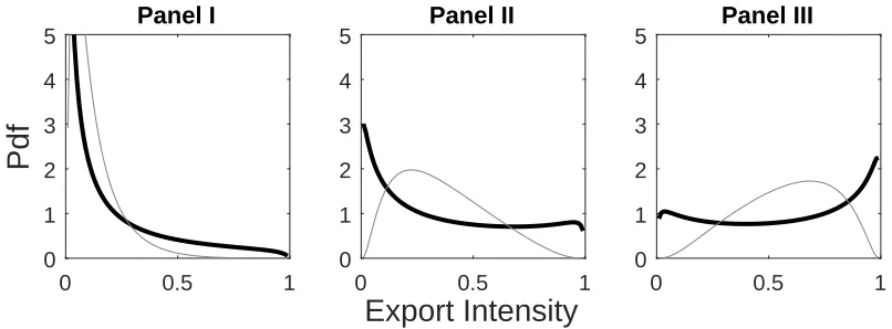
lowers the ratio sd{sx.22 Figure 3 shows how the distribution of export intensity changes as the

relative size of the foreign market increases (when moving from Panel I on the left to Panel III on the right). The darker line shows the distribution of export intensity when revenue shifters are

lognormal and the sum of their variances is equal to 4 —thus, producing a bimodal distribution—

while the lighter line represents a unimodal distribution (i.e. when σ_zd2 `σ_zd2 “1).

Figure 3: Reduction in Export Costs with and without Twin Peaks

0 0.5 1

0 1 2 3 4 5

Pdf

Panel I

0 0.5 1

Export Intensity

0 1 2 3 4

5 Panel II

0 0.5 1

0 1 2 3 4

5 Panel III

The figure plots the probability density function of export intensity when revenue shifters are lognormal withσ2

zd` σ2zd “4 (darker line) andσ

2

zd`σ

2

zd “1 (lighter line) for different values of the ratio of scale parameters; namely, sd{sx“0.1 in Panel I, 0.5 in Panel II and 1.5 in Panel III.

In panel I of Figure 3, trade costs are so high that most exporters sell only a small share of their

output abroad regardless of the level of dispersion in revenue shifters, and therefore, the two ex-port intensity distributions look quite similar.23 _{As trade costs fall, the intensity of all exporters}

increases and the distribution of export intensity shifts to the right. However, the difference in

the distribution with and without twin peaks also becomes starker. When the variance of revenue shifters is sufficiently large to generate twin peaks, greater access to foreign markets increases the

prevalence of high-intensity exporters; conversely, when the dispersion is unimodal, the increase in

the intensity of exporters following liberalization is gradual.

Exports and Firm-level Volatility. A recent literature investigates how exporting affects

firm-level volatility (see e.g. Ria˜no,2011;Vannoorenberghe,2012;Kurz and Senses,2016;Girma et al.,

2016). In principle, exporting allows firms to diversify demand shocks that are not perfectly

corre-lated across markets, thereby lowering the volatility of sales.

We now show that the existence of twin peaks in the distribution of export intensity reduces the

22_{If both countries are symmetric in size and the reduction in trade costs is bilateral, this direct effect coincides with}

the full general equilibrium change in relative market size. More generally, a lower trade cost also affects wages and price indices in both countries. Demidova and Rodr´ıguez-Clare(2013) show that is not possible to unambiguously sign the effect of trade liberalization on wages and price indices in theMelitz(2003) model when countries are asymmetric in terms of size unless the model is parameterized and fully solved.

23

To fix ideas, assume that the foreign country is twice as large as home, i.e.Ax{Ad“2. Then, asd{sx ratio of

diversification benefits of exporting. To do so, we introduce a minor modification to the revenue

functions defined in (2). We assume that aggregate variables, productivity and firm-destination-specific revenue shifters are time-invariant, but sales vary over time in response to idiosyncratic

i.i.d. demand shocks, itpωq, which are drawn from a distribution with mean 1 and variance ν_i2

—the same set up considered byVannoorenberghe(2012). Thus, firmω’s sales in marketiP td, xu

in periodtare given by:

ritpωq “Φpωq ¨si¨zipωq ¨itpωq. (9)

Since shocks are multiplicative and transitory, the firm chooses the same optimal prices as in the

static model described before, and therefore, Epωq “ _Z Zxpωq

dpωq`Zxpωq —the same expression as (3)— now denotes firm ω’s long-run export intensity.

Assuming that demand shocks are equally volatile across markets, it can be shown that firms’

volatility is minimized when the firm’s long-run export intensity equal 0.5.24 If the distribution of long-run export intensity displays twin peaks, a greater dispersion of revenue shifters increases the share of firms with export intensity close to 0 and 1. As a result, the aggregate volatility-reduction

effect of exporting is weakened because most exporters sell the majority of their output either

domestically or abroad.

4

Estimation

In the previous section we showed that the distribution of export intensity is fully characterized by

the shape parameter governing the distribution of firm-destination-specific revenue shifters and a country’s relative size with respect to the rest of the world. We now discuss how we estimate these

parameters using the cross-country firm-level data from the WBES.

Identification Strategy. We first present a result that greatly facilitates the identification and

estimation of the parameters governing the distribution of revenue shifters. Namely,

Proposition 3. If revenue shifters are independent across firms and destinations and follow either

lognormal, gamma, or Fr´echet distributions as specified in Proposition 1, then the median export intensity, emed, is given by:

emed“ sx

sd`sx

, (10)

which is independent of the shape parameter of revenue shifters.

Proof. See AppendixA.3.

24

In AppendixBwe show that the volatility of the growth rate of total sales for firmω, Volpωq, is given by:

Volpωq «2“p1´Epωqq2¨νd2` pEpωqq

2

¨ν2x

‰ .

The volatility of sales is therefore minimized when the firm’s long-run export intensity is equal to νx2 ν2

d`νx2

Thus, Proposition 3allows us to recover the relative market size for each country directly from

the export intensity data by inverting equation (10):

ˆ

sd

sx

˙

“ 1´e med

emed . (11)

It also follows from (11) that our measure of relative market size is invariant to the underlying distribution of revenue shifters. Crucially, Proposition 3 allows us to recover relative market sizes

without having to estimate or calibrate other parameters of the model such as trade costs, or the

parameters characterizing the productivity distribution, all of which are necessary to compute the value of si when solving the model explicitly.

Conditional on relative market size, the identification of the shape parameter is straightforward.

The value of this parameter is determined by whether the mass of the export intensity distribution is concentrated in the interior or near the boundaries of the support. If the dispersion of revenue

shifters is low, then the distribution of export intensity is unimodal, with most exporters exhibiting

an intensity close to sx

sd`sx. On the other hand, if there large clusters of exporters with intensities near 0 and 1, then the dispersion of revenue shifters will be sufficiently high so that the shape

parameter satisfies the conditions spelled out in Proposition2.

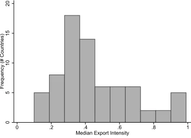
Scale Parameters. Figure4displays the distribution of the median export intensity in our data.

Although there is large variation across countries, the median export intensity ranges between 0.2

and 0.8 for most of them. In the lower end of the distribution, Brazil and Russia have a median export intensity of 0.1, while at the other extreme, Bangladesh, Madagascar, Morocco, Pakistan,

Philippines and Sri Lanka all have a median export intensity greater than 0.9. Summary statistics

for the relative country size implied by countries’ median export intensity are reported in Table4. For the median country in our sample, the domestic market is 50% larger than the foreign market.

Figure 4: Distribution of Median Export Intensity Across Countries

0

5

10

15

20

Frequency (# Countries)

0 .2 .4 .6 .8 1

Median Export Intensity

Table 4: Inferred Relative Domestic Market Size

Mean Percentile

5 25 50 75 95

xsd

sx 1.967 0.010 0.667 1.500 2.333 5.667

Country-Specific Shape Parameters. We first estimate country-specific shape parameters for each of the three revenue-shifter distributions that we consider. These are estimated by maximum

likelihood conditional on relative market size being given by (11). Our objective is to determine

whether the conditions for bimodality of the export intensity distribution that we identified in Proposition2bear out in the data. With our estimates at hand we then use theVuong(1989) test

to compare the resulting distributions in terms of their fit to the data. Vuong (1989) proposes a

likelihood-ratio (LR) based statistic based on the Kullback-Leibler information criterion to measure the closeness of a model to the true data generating process.25 This test has two desirable properties for our purposes: first, it can be used to compare non-nested econometric models —in particular those that are obtained from different families of distributions, as in our case. Second, the test is

directional —i.e. it indicates which competing model is better when the null hypothesis that two

models are indistinguishable from each other is rejected.

It is important to note that the export intensity pdfs we derive are not defined at an export

intensity of 1 —in other words, they do not admit firms exporting all their output. Since ‘pure

exporters’ are ubiquitous in the data, we need to censor their export intensity, and we do so at a conservative value of 0.99. Increasing the censoring cutoff biases the shape parameter in the

direction of bimodality (i.e. lowers the shape parameter for gamma and Fr´echet and increases the

sum of variances in the lognormal case). This is the case because the distribution of revenue shifters would need to generate large shares of extremely low and high realizations to be able to reproduce a

significant number of exporters with intensity at or above the censoring threshold.26 To ensure that our results are not driven by our chosen censoring threshold, we re-estimate the shape parameter dropping all pure exporters in the robustness analysis in the next section.

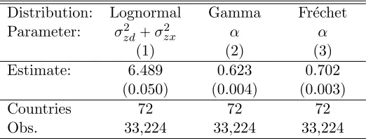
The country-specific shape parameter estimates are reported in Table C.1in Appendix C. In

all but a handful of cases they imply export intensity distributions that are bimodal. The mean estimates across countries are 6.489 for lognormal and 0.672 and 0.740 for gamma and Fr´

echet-distributed revenue shifters respectively. In the lognormal case, all shape parameters satisfy

con-ditions (7) and (8) for bimodality (see Figure A.5in Appendix A.2.1). When revenue shifters are distributed gamma or Fr´echet, we estimate shape parameters greater than 1 for 6 and 7 countries

respectively —all of which are identified as unimodal by the dip test reported in Figure 2.

25

Mr´azov´a et al.(2015) also use the Kullback-Leibler divergence to evaluate how different combinations of demand functions and productivity distributions fit the size distribution of French firms exporting to Germany.

26_{For instance, for a firm to have an export intensity of 0.99, its export revenue shifter has to be 99 times larger}

The results of the Vuong (1989) test reported in columns (1)-(3) and (7)-(9) of Table D.1 in

AppendixDdo not suggest that one of the underlying distributions of revenue shifters clearly dom-inates the others in terms of fitting the data. Comparing the lognormal-based export intensity with

the gamma and Fr´echet distributions reveals that in 20 countries we cannot discriminate between

the two competing models, while the remaining ones are evenly split between the lognormal and the competing distribution. Among the set of countries for which lognormal performs worse than

the alternative, gamma fits the data better than Fr´echet in all but two countries.27

Single Shape Parameter. The results discussed above show that large heterogeneity in firms’

performance across domestic and export markets can successfully explain the occurrence of twin

peaks. We now investigate if our model can account for the variation we observe in the distribution of export intensity across countries. Putting it differently, can our model explain the patterns

depicted in Figure1?

To answer this question we consider a scenario in which firms in all countries draw revenue shifters in each destination they serve from a distribution with the same shape parameter. This

implies that the variation in the distribution of export intensity across countries is entirely due to

differences in relative market size. In order to estimate this ‘restricted’ model, we pool data across all countries and weight each observation by the inverse of the number of observations available for

each country.

The estimates for the single-shape parameter models are reported in Table 5. The

point-estimates are very similar to the average across the country-specific point-estimates reported above and

all imply a bimodal distribution of export intensity. Notably, the Vuong test reveals that for approximately two-thirds of the countries we cannot discriminate between the restricted model and

the one where shape parameters are country-specific (see columns (4)-(6) and (10)-(12) of Table

D.1in AppendixD), even though the latter fits the data better by definition. The restricted model has the additional advantage that it greatly facilitates conducting the robustness analysis below in

which we investigate whether the existence of a second mode near 1 is driven by specific subsets of

firms being particularly export intensive.

Using customs-level data from France and the World Bank’s Export Dynamics Database,Eaton

et al. (2011) and Fernandes et al. (2015) estimate structural models of trade that incorporate

lognormally-distributed firm-destination-specific revenue shifters. Although their models are richer than ours —including, for instance, shocks to productivity and fixed costs and convex marketing

costs— they both find that the variance of revenue shifters is large enough to generate bimodality

in our model.28

27_{When the Vuong test indicates that lognormal dominates gamma it also suggests that the former provides a}

better fit to the data than Fr´echet. The only exception is in the case of Uganda in which the test rejects gamma in favor of lognormal but cannot discriminate between lognormal and Fr´echet.

28

Table 5: Single Shape Parameter Estimate

Distribution: Lognormal Gamma Fr´echet

Parameter: σ2

zd`σ2zx α α

(1) (2) (3)

Estimate: 6.489 0.623 0.702

(0.050) (0.004) (0.003)

Countries 72 72 72

Obs. 33,224 33,224 33,224

The table reports the maximum likelihood estimate of the shape param-eter governing firm-destination-specific revenue shifters for different un-derlying distributions, conditional on sx{sd being given by (11). The

pdf used in the estimation are given by equations (4), (5), and (6), for lognormal, gamma and Fr´echet distributed revenue shifters respectively. Standard errors are reported in parentheses.

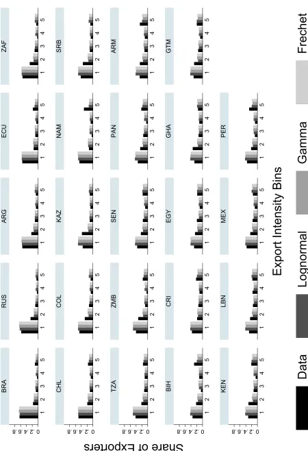
Figure 5 presents the fit of the three restricted models to the data, with countries sorted

according to their estimated relative market size. Relying only on variation in countries’ relative market size and a unique shape parameter governing firm-destination revenue shifters, our model

reproduces closely the wide range of shapes observed in the distribution of export intensity across the world: unimodal distributions where the majority of exporters exhibit either very low or very

high export intensity, just as well as those displaying twin peaks. Figure 5 also echoes the results

of the Vuong test discussed above —all three distributions of revenue shifters, lognormal, gamma and Fr´echet, fit the export intensity data quite well.

Relative Country Size and Bimodality

We have established that when the conditions in Proposition 2 are satisfied, the distribution of

export intensity is bimodal. Nevertheless, Figure 2 shows that one-third of the countries in our sample have a unimodal distribution. These two are reconciled in our model by noting that as

relative market size either becomes too small or too large, the height of the minor mode shrinks

enough for the distribution to appear unimodal. In these circumstances, a statistical test of uni-modality, such as the dip test, is likely to not reject the null hypothesis of unimodality. That is,

the probability that the test produces a Type-II error increases.

Figure 6 plots the dip statistic calculated for data simulated using the shape parameters reported in Table 5 for different values of the median export intensity. Figure 6 shows that there is an

inverse-U relationship between the dip statistic (recall that a larger number means that the dis-tribution is less likely to be unimodal) and the median export intensity. Countries that are either

very small or very large relative to the rest of the world —which have very high and low median

export intensities respectively— are likely to be classified as unimodal by the dip test (dashed lines in Figure6); conversely, countries for which the domestic and export markets are more similar in

Figure 5: Mo del Fit Exp ort In tensit y Distribution 0.2 .4.6

.8 .8 .4.6 0.2 .8 .4.6 0.2 .8 .4.6 0.2 .8 .4.6 0.2

1 2 3 4 5 1 2 3 4 5 1 2 3 4 5 1 2 3 4 5 1 2 3 4 5 1 2 3 4 5 1 2 3 4 5 1 2 3 4 5 1 2 3 4 5 1 2 3 4 5 1 2 3 4 5 1 2 3 4 5 1 2 3 4 5 1 2 3 4 5 1 2 3 4 5 1 2 3 4 5 1 2 3 4 5 1 2 3 4 5 1 2 3 4 5 1 2 3 4 5 1 2 3 4 5 1 2 3 4 5 1 2 3 4 5 1 2 3 4 5 BRA RUS ARG ECU ZAF CHL COL KAZ NAM SRB TZA ZMB SEN PAN ARM BIH CRI EGY GHA GTM KEN LBN MEX PER

Data

Lognormal

Gamma

Frechet

Share of Exporters

Figure 5: Mo del Fit Exp ort In tensit y Distribution, Con tin ued 0.1 .2.3

.4 .4 .2.3 0.1 .4 .2.3 0.1 .4 .2.3 0.1 .4 .2.3 0.1

1 2 3 4 5 1 2 3 4 5 1 2 3 4 5 1 2 3 4 5 1 2 3 4 5 1 2 3 4 5 1 2 3 4 5 1 2 3 4 5 1 2 3 4 5 1 2 3 4 5 1 2 3 4 5 1 2 3 4 5 1 2 3 4 5 1 2 3 4 5 1 2 3 4 5 1 2 3 4 5 1 2 3 4 5 1 2 3 4 5 1 2 3 4 5 1 2 3 4 5 1 2 3 4 5 1 2 3 4 5 1 2 3 4 5 1 2 3 4 5 POL SYR UGA UKR UZB BOL KOR URY BLR CHN HRV HUN IND IRL MYS NIC PRY SLV TUR SVK ETH CZE HND KGZ

Data

Lognormal

Gamma

Frechet

Share of Exporters

Figure 5: Mo del Fit Exp ort In tensit y Distribution, Con tin ued 0.2 .4.6

.81 .81 .4.6 0.2 .81 .4.6 0.2 .81 .4.6 0.2 .81 .4.6 0.2

1 2 3 4 5 1 2 3 4 5 1 2 3 4 5 1 2 3 4 5 1 2 3 4 5 1 2 3 4 5 1 2 3 4 5 1 2 3 4 5 1 2 3 4 5 1 2 3 4 5 1 2 3 4 5 1 2 3 4 5 1 2 3 4 5 1 2 3 4 5 1 2 3 4 5 1 2 3 4 5 1 2 3 4 5 1 2 3 4 5 1 2 3 4 5 1 2 3 4 5 1 2 3 4 5 1 2 3 4 5 1 2 3 4 5 1 2 3 4 5 NGA SVN SWE MUS JOR BGR LTU MDA THA IDN EST ALB LVA MKD TUN ROU VNM LAO PAK BGD LKA MAR MDG PHL

Data

Lognormal

Gamma

Frechet

Share of Exporters

Figure 6: Relative Market Size and Bimodality of the Export Intensity Distribution

0 0.1 0.2 0.3 0.4 0.5 0.6 0.7 0.8 0.9 1

Median Export Intensity

0 0.01 0.02 0.03 0.04 0.05 0.06

Dip Test of Unimodality

Lognormal

Fréchet

Gamma

The figure reports the value of the dip test statistic calculated on simulated export intensity draws using the estimated shape parameters reported in Table5for different values of the median export intensity. Solid lines repre-sent sets of draws in which the null hypothesis of unimodality is rejected at the 1% significance level, while dashed lines show the realizations for which unimodality is not rejected.

Figure 7: Prevalence of Bimodality and Median Export Intensity across Countries

ARG

COL BGDLKA

RUS ZAF POL

BRA KAZSRBTZA LBNMEXUKR CZE BLR

SYR MYS IDN

CHL SENGHAKOR

ECU EGY THA EST MDGMAR

HUN

CRI HRV KGZSWE VNMLAO PHL ZMB UZBKEN SVN BGRMDA

SVK PAK

PRY

GTM NGA LTU ROU

UGA TUR

ARMBOL URY JOR PANBIHPER NIC MKDLVA

ETH CHN SLV

TUN HND

IND IRL

MUS

NAM ALB

.02

.04

.06

.08

.1

.12

Dip Test Statistic of Unimodality

0 .2 .4 .6 .8 1

Median Export Intensity

95% CI Fitted values

Unimodal Bimodal

The figure plots the fitted values obtained after regressing each country’s dip test statistic (reported in Table2) on a country’s median export intensity and median export intensity squared. The estimated equation isdip“0.0086

p0.0096q`

0.2044

p0.0326q

median´0.1736

p0.0397q

median2_{, and}

Figure 7 reveals that the inverted-U pattern is also clearly borne in the data. Thus, the high

dispersion in firm-destination-specific revenue shifters is able to explain why the distribution of export intensity is bimodal in some countries but appears unimodal in others. Figure5shows that

relative country size clearly determines whether a country has uni- or bimodal distribution.

5

Robustness

An alternative explanation for the existence of twin peaks is that they are the product of a

compo-sition effect arising from certain groups of firms having markedly different export intensities. Thus, in this section we probe the robustness of our single-shape-parameter estimates by excluding

differ-ent subsets of firms that the literature has iddiffer-entified as being more export-oridiffer-ented than average.

These results are reported in columns (2)-(7) of Table 6 (column (1) reproduces our benchmark single-shape parameters estimates for convenience). Notice that as we restrict the sample across

dif-ferent specifications, the median export intensity changes for each country relative to the estimates

presented in Figure4.

Foreign Ownership. We start our analysis by excluding firms that are foreign-owned —i.e. those with a share of foreign equity of at least 10%— from the estimation. AsAntr`as and Yeaple(2014)

note, multinational firm affiliates tend to be more export intensive than non-multinational firms

because of intra-firm vertical specialization taking place between parent companies and affiliates.

Arnold and Javorcik (2009) find that the export intensity of Indonesian plants that are acquired

by foreign investors increases substantially after acquisition.

Export Processing. Firms engaged in export processing activities have also been identified as

being highly export intensive (see e.g.Brandt and Morrow,2017). Export processing occurs when a

producer ships an unfinished product to a foreign country where some value-added is incorporated into it before being re-exported again. Firms undertaking processing activities have high export

intensity because the tariff concessions available in this customs regime require firms to export all goods that incorporate duty-free imported inputs. Although the WBES data does not identify firms

that export through a processing custom regime explicitly, we use the share of intermediate inputs

accounted for by imports to construct a proxy for export processing. Therefore, we classify firms as processing exporters if their share of imported inputs exceeds 90% of their total expenditure in

intermediate inputs.

Pure Exporters. In our most stringent exercise, we exclude firms that export all their output

—‘pure exporters’— from the estimation. In the model we proposed in Section3, we assumed that

all firms pay a fixed costfd to set up a plant, and then, additionally, a fixed costfx if they choose

to export. Therefore, all operating firms would sell a positive quantity of output —no matter how

small— in the domestic market. Alternatively, firms could face destination-specific fixed costs,

T able 6: Robustness Chec ks F ull Excluding Coun tries Sample F oreign Pro cessing Pure Exp. without ESR OECD non -OECD (1) (2) (3) (4) (5) (6) (7) Lognormal σ

2 zd

`

σ

2 zx

the latter model, firms with relatively low productivity but facing sufficiently high demand abroad

would choose to operate as pure exporters.

The results reported in columns (2)-(4) of Table 6 show that the estimated shape parameters

are extremely robust, and they all imply a bimodal distribution of export intensity. Excluding pure exporters produces the largest reduction in the dispersion of revenue shifters as it directly affects

the export intensity distribution. The important thing, however, is that even when we exclude

these firms, which account for a substantial share of high-intensity exporters, our main result re-mains unchanged. Having examined firm-level characteristics, we now turn to country-level factors

that could potentially generate bimodal export intensity distributions through a composition effect.

Subsidies with Export Share Requirements. The use of incentives subject to export share

requirements distorts a country’s ‘natural’ export intensity distribution because firms are induced

to operate at a higher export intensity than the one they would have chosen otherwise. Defever and Ria˜no(2017a) show that this can produce large negative welfare effects in countries enacting them.

As we have noted in Section2, approximately half of the countries in our data provide this class of

incentives. ESR are frequently imposed in special economic zones —geographically-bounded areas in which customs, tax and investment regulations are more liberal than in the rest of the country

(Farole and Akinci, 2011; Defever et al., 2016). By excluding countries that offer subsidies with ESR from our estimation we seek to allay the concern that the high prevalence of twin peaks across

the world is due to the use of these incentives.

Level of Development. Although our sample consists primarily of developing countries, we also

investigate if there are significant differences in the estimated shape parameter between OECD and

non-OECD countries. If, for instance, the high prevalence of high-intensity exporters is caused by vertical specialization driven by cross-country wage differentials, then it could be the case that the

value of the shape parameter is influenced by the composition of countries in our sample.

The results presented in columns (5)-(7) of Table6show, once again, that the estimated shape

parameters imply bimodality. Excluding countries that provide subsidies with ESR, which are also

countries where high-intensity exporters are ubiquitous, has a similar effect on the shape parameter as excluding foreign-owned and export processing firms. Consistent with the intuition outlined

above, the dispersion of revenue shifters is higher for developing countries than for developed ones.

Sectoral Differences. Bernard et al.(2007) document large differences in average export intensity

across manufacturing industries in the U.S. Thus, we now explore the possibility that a country’s bimodal export intensity distribution is the result of a mixture of sectoral distributions, which may

differ substantially due to technological differences or comparative advantage. For this exercise we