Dynamic exergy analysis for the thermal storage optimisation of the building envelope

Dynamic Exergy Analysis for the Thermal Storage

Optimization of the Building Envelope

Valentina Bonetti1,* and Georgios Kokogiannakis2

1 _{Energy Systems Research Unit (ESRU), University of Strathclyde, Glasgow G1 1XJ, UK}

2 _{Sustainable Buildings Research Centre (SBRC), University of Wollongong, Wollongong, NSW 2500,}

Australia; [email protected]

* Correspondence: [email protected]; Tel.: +44-(0)141-548-3986

Academic Editors: Kondo-Francois Aguey-Zinsou, Da-Wei Wang and Yun-Hau Ng Received: 1 September 2016; Accepted: 22 December 2016; Published: 13 January 2017

Abstract:As a measure of energy “quality”, exergy is meaningful for comparing the potential for thermal storage. Systems containing the same amount of energy could have considerably different capabilities in matching a demand profile, and exergy measures this difference. Exergy stored in the envelope of buildings is central in sustainability because the environment could be an unlimited source of energy if its interaction with the envelope is optimised for maintaining the indoor conditions within comfort ranges. Since the occurring phenomena are highly fluctuating, a dynamic exergy analysis is required; however, dynamic exergy modelling is complex and has not hitherto been implemented in building simulation tools. Simplified energy and exergy assessments are presented for a case study in which thermal storage determines the performance of seven different wall types for utilising nocturnal ventilation as a passive cooling strategy. Hourly temperatures within the walls are obtained with the ESP-r software in free-floating operation and are used to assess the envelope exergy storage capacity. The results for the most suitable wall types were different between the exergy analysis and the more traditional energy performance indicators. The exergy method is an effective technique for selecting the construction type that results in the most favourable free-floating conditions through the analysed passive strategy.

Keywords:dynamic exergy analysis; building envelope; energy storage

1. Introduction

Exergy is a state function that combines the first and second law of thermodynamics through a reference environment. The strong dependency of exergy from the defined reference creates a “co-property” of the system and the environment [1] and enables a quantification of energy quality, measured as “the maximum theoretical useful work obtainable as the system interacts to equilibrium, heat transfer occurring with the environment only” [2]. A simple way to obtain exergy fluxes is to apply “quality factors”q f as conversion factors of the energy fluxes. For example, in the case of a conductive heat transferQoccurring at a constantT, if the reference environment has temperatureT0, the associated exergy transferBis directly derived from the Carnot efficiency as:

B(Q) =q f ·Q=

1−T0

T

·Q, (1)

Other types of energy exchanges have higher quality factors, which means that a greater portion of the energy flux can be converted into useful work (for instance, electricity has a quality factor of one).

Exergy analysis represents an established technique in the process optimization of many engineering fields, for example of thermal power plants, and as thoroughly explained in the IEA

Annex 49 report [3], it is a potentially useful technique to also promote a more rational use of energy resources in the built environment. The quality of the energy contained in a comfortable room is fairly low, because the indoor temperatures are around 20◦C, which corresponds to a quality factor of 7% if the reference temperature is 0◦C. However, in this case, the overall energy demand of the building is often satisfied with a much higher quality source of energy supply.

Understanding and quantifying energy quality (exergy) is crucial for a rational use of limited resources, where supplies and demands are properly matched to reduce waste. However, the application of the exergy approach to building design is still very limited. Major obstacles for the dissemination of building exergy analysis are its complexity, the controversial definition of the reference state [4] discussed in Section2.2.3and a lack of dynamic exergy simulation tools (some of which are described in [3]). Furthermore, the building envelope, which is the last element of the energy chain shown in Figure1, is not considered in detail, to the authors’ best knowledge, in any guideline or case study in the literature.

Figure 1.Energy and exergy flux through the building energy chain (adapted from [3]) with permission from the Fraunhofer Institute for Building Physics, 2011.

On the other hand, the interaction between buildings and their surrounding environment is often not optimal. One common problem is constituted by the summer performance of building constructions located in climates with hot days and relatively low nocturnal temperatures (like the Mediterranean). The role of thermal mass in lowering the cooling load of buildings is largely documented (e.g., in [5–8]), but not systematically and quantitatively acknowledged in current practice. The inner part of the envelope of modern buildings is generally not designed to absorb and release all of the internal and solar gains in a daily cycle, and air-conditioning is the usual solution to address the occurrences of overheating. Low nocturnal outdoor temperatures are barely exploited as they were in traditional architecture.

2. Methods and Materials

This research is focused on the potential for thermal storage in the envelope. The guidance provided by the energy analysis typically performed to select the envelope during the design phase, discussed in Section2.1, is compared to the support offered by a tailored exergy assessment (presented in Section2.2) for the case study described in Section2.3representing a common example in the Mediterranean climate.

2.1. Energy Analysis

In a typical workflow, the energy analysis in support of the design process is conducted according to the methods recommended in the official Italian guidelines [10] (described in [11]) and [12], as derived from European directives. The following indicators are commonly used:

• steady-state energy performance:

– U-value (U; (W/m2K)) – mass per area (Ma; (kg/m2))

– thermal capacity per area (Cta; (kJ/m2K)) – monthly energy demand data

• dynamic energy performance:

– decrement factor (f) – time lag (τ; (h))

In a few cases, further calculations are performed, such as:

• dynamic energy performance:

– indoor admittance modulus (Yiimodulus; (W/m2K)) – indoor admittance phase (Yiiphase; (h))

Simulation data (such as temperatures and consumptions) from a dynamic energy software are rarely obtained because they are not required by Italian building regulations.

In this study, seven different realistic construction types, detailed in AppendixA, are compared on the basis of the envelope indicators generally used in a preliminary energy assessment (U-value, decrement factor, time lag, mass per area, static thermal capacity, indoor admittance). Thereafter, the different types are ranked according to the following indicators that are mainly considered for envelope selection during the summer performance evaluations: decrement factor f and time lagτ. 2.2. Exergy Analysis

2.2.1. The Exergy Balance

The theoretical framework of this study, as extracted and adapted by the proposal of Pons [4] considers a simplified system working as storage and where the boundaries of the following three fluxes occur in a cyclic process of charging and discharging: a power inputp, a useful effectu, for instance heat subtraction, and an energy exchange with the environmentenv. The instantaneous formulations of the first and second law of thermodynamics, in terms of energy (e) and entropy (s) rates, are:

(

ep+eu+eenv=E˙

in which ˙Eand ˙Srepresent the rate of energy and entropy stored in the system, respectively (null for stationary processes), and ˙Psthe instantaneous production of entropy. If the ratio of entropy-energy (which is often, but not always, approximately constant) of the generic fluxxis calledrx=sx/ex, the system (2) becomes:

(

ep+eu+eenv =E˙

rpep+rueu+renveenv+Ps˙ =S.˙ (3)

For example, for fluxes like work or electricity, the associated entropy is null, and thus,rx=0; for a constant-temperature, heat flow (transferred through a boundary atTx) isrx=1/Tx.

Exergy is the linear combination of energy and entropy through a constant reference temperature T0; the instantaneous exergy balance is thus obtained by multiplying the second equation of (3) byT0 and then subtracting the result from the first equation of (3):

ep(1−T0rp) +eu(1−T0ru) +eenv(1−T0renv) = (E˙−T0S˙) +T0Ps.˙ (4) The energy termseare multiplied by the term(1−T0rx), the so-called “quality factor”, to obtain exergy flows on the left-hand side, while the right-hand side represents the system state variation, which is composed of the exergy storage and the exergy losses due to irreversibilities. IntroducingB as the notation for exergy andbfor exergy flow rates, Equation (4) becomes:

bp+bu+benv=B˙+irreversibilities. (5) where ˙Bis the exergy variation rate of the system. Time integration in the generic interval[0,t∗]

leads to:

Ep(1−T0rp) +Eu(1−T0ru) +

Z t∗

0 eenv

(1−T0renv)dt−

Z t∗

0 T0 ˙ Psdt=

Z t∗

0 ˙ Edt−T0

Z t∗

0 ˙

Sdt. (6)

in whichrp andru are considered constant, but renv, and thus, the environmental quality factor 1−T0renvis potentially variable, which means that the exergy extracted from the environment can have a fluctuating quality.

In a cyclic process, exergy content variations (the right-hand side of Equation (6)) are null after a period or negligible for a non-perfect cycle. The exergy balance over a cycle is therefore:

Ep(1−T0rp) +Eu(1−T0ru) +

I

eenv(1−T0renv)dt≈

I

T0Ps˙ dt. (7)

The first term on the left side of Equation (7) is the exergy input from the generic power source (its main distinctive feature being a non-zero monetary value); the second term represents the useful effect (for example, the coverage of the building thermal demand); and the third term is the exergy exchanged with the environment; on the other side, the exergy is destroyed by irreversibility. In synthesis, Equation (7) can be written as:

Bp+Benv+Bu ≈irreversibilities. (8)

2.2.2. The Exergy Balance Applied to the Building Envelope

In the case of the building envelope, the useful effectBuis the coverage of heating or cooling loads and, thus, the satisfaction of the corresponding building “exergy demand” (Bdemand), of the opposite sign. The balance (8) can therefore be written as:

The complication of the balancing Equation (9) when applied to the building envelope is thatBenv andBdemandare not distinctly distinguished a priori: the spontaneous interaction with the environment, together with internal loads, is the cause of the exergy demandBdemand, which therefore has the same provenance of the termBenv. However, the reason for having two separate contributions lies in the different steps in which the design process can be subdivided:

1. envelope exergy demand (Bdemand) reduction 2. exergy extraction from the environment (Benv) 3. power input and irreversibility (H

T0Ps) optimization˙

The final aim is to reduce the need of the power exergy inputBp. The first step is the application of classical conservation measures, for example appropriate envelope insulation or shading devices, in order to achieve indoor “free-floating” conditions (which means in absence of HVAC systems) that are as near as possible to thermal comfort. In many cases, thermal comfort is not achieved with simple measures, and an exergy input is still required. The second step tries to answer the question: how much of the demanded exergy can be actually extracted by the same surrounding environment and how? This second step, which is the focus of the present study, analyses the free-floating behaviour of the building in depth and precedes any decision about the power source possibly needed to achieve thermal comfort. The last step, if required, involves the design of power input systems and their optimisation, which deserves a deeper discussion, and it is not included in this study. It is worth noting that maximising the exergy extraction from the environment does not coincide with irreversibility minimisation and, on the contrary, can even lead to a more irreversible system; however, buildings are not machines, and irreversibility and sustainability are not necessarily counterposed if carbon-based sources are not involved. This discussion is out of the reach of the present investigation and constitutes the focus of further research.

2.2.3. The Reference TemperatureT0

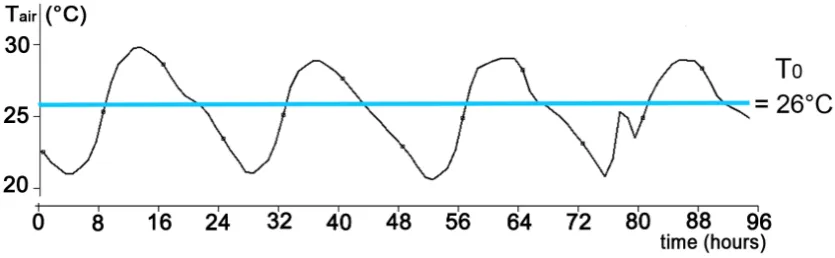
The reference temperature for dynamic exergy analysis is a highly controversial issue, and no consensus has yet been reached on the most suitable choice. Pons [4] demonstrated analytically that a variable reference state corresponding to the outdoor air temperatureTair(used by the vast majority of authors) leads to a path-dependent “exergy”, which is no longer a function of state, and thus, it cannot be used as such. A comparison between variable and fixed references used for the dynamic exergy analysis of this study pointed out that the fluctuating value of the external temperature brings perplexing results about exergy storage, as opposed to the ones obtained with a fixed reference, which are sound and easy to interpret.

In this research, the constant valueT0 = 26◦C is therefore used as the reference temperature. Pons [4] suggests the use of the “most favourable” temperature for the considered process that is available in the surrounding environment. For a standard cooling system, the most favourable choice would be the minimum value of the ambient air temperature Tair in the assessed period (T0=min(Tair(t))). However, the aim is to minimise the envelope exergy demand and consequently to maximise exergy harvesting from the environment whenever possible.

period of this study, as can be observed in Figure2, which reports the ambient air temperatures for the period 17–20 of August of the climate file.

Figure 2.Outdoor air temperatureTairtrend (Rome) and constT0in case study days (17–20 August).

2.2.4. A Simplified Model for Nocturnal Ventilation as a Cooling Strategy

A detailed analysis with a dynamic exergy simulator would be needed to assess every term of the exergy balance (7) and gain a deeper insight into the interactions between the building and its environment, but no dynamic exergy tools are directly available yet. However, a simpler model, focused on the most relevant phenomena in the investigated case, can be used to understand the potentialities of exergy analysis in this context, and it is thus adopted.

The aim of the proposed analysis is to provide support to the second design step mentioned in Section2.2.2, the enhancement of the extraction of useful exergy from the surrounding environment. The easiest and potentially lease expensive option is considered as a simple example for demonstrating the design process: the environmental exergybenvis extracted only from the outdoor air by means of nocturnal natural ventilation and stored in the building envelope, neglecting all other possibilities (e.g., an exchange with the ground).

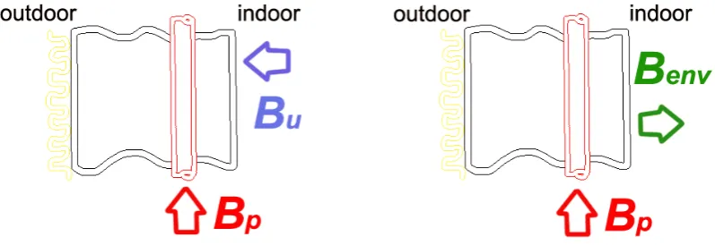
The typical summer cycle can be divided into two main periods: day and night. During the day, the exergyBufrom cooling loads is adsorbed by the wall interior surfaces until the maximum storage point (left part of Figure3); then, the indoor temperature tends to rise, and a power inputBpis needed to maintain comfort. During the night, when the outdoor air temperature is below the comfort setpoint (right part of Figure3), heat can be released from wall interior surfaces to fresh air introduced inside the thermal zone (which corresponds to the exergyBenvextracted from the ventilation air); a power inputBpis generally not needed in this phase, but could be requested in some cases (for example, if the time constant of the distribution system is high or in case of off-peak demand strategies). The power source selection and its distribution system, symbolically represented by embedded pipes in Figure3, are not discussed in this study, since they constitute the focus of the third design step.

In this simplified case, the useful effectBu of Equation (8) is subtracting the cooling demand Edemandat a generic demand temperatureTdemand, which depends on the distribution system adopted; the daily exergy balance therefore becomes:

Ep(1−T0rp) +

I

qair

1− T0

Tair

dt≈Edemand

1− T0

Tdemand

+

I

T0Ps˙ dt, (10) in which the cooling loads representing an exergy output (negative) become a positive exergy demand on the right-hand side, and the environmental resourceenvunder investigation is air (eenv=qair: heat exchanged by convection at temperatureTair;renv = 1/Tair). The 24-h cycle is split into two parts, cool-exergy storage charging (at night, zone unoccupied) and discharging (daytime, zone occupied).

The main hypotheses are:

• decrement factor and time lag are such that the transmission through the wall is negligible when considering storage effects

• the analysed thermal zone is unoccupied during nocturnal periods of natural ventilation (comfort requirements can thus be relaxed, and air velocity can exceed comfort limits)

• the indoor temperature can be maintained at outdoorTairthrough high-rate ventilation (10 air changes per hour (ACH) or more) if needed.

Figure 3.Envelope simplified fluxes: during the summer day, the useful effectBuis represented by the absorption of internal gains (on the left), whilst during the night,Benvis released to the external air by means of increased ventilation (on the right). The power inputBp, if needed, is delivered by the distribution system (here represented by the embedded red pipe).

The most relevant phenomena become the daytime absorption of internal and solar gains and the nocturnal release of the energy accumulated in the thermal mass. The simplified model consists of a closed system whose boundaries are the middle section of the wall (considered as completely insulated from the exterior) and a parallel layer inside the thermal zone, where the temperature reaches the room value.

The second design step consists of maximising the exergy extracted from ambient air when its temperature is sufficiently low. In this case, the power input exergy required to facilitate the exchange should be null or lower thanBair. This translates in an objective function, the cool exergy of external air, to be maximised over the night (whenTair<T0):

Bair =

I

qair

1− T0

Tair

dt (11)

In this simplified case, the objective Function (11) is calculated for a significant sample of the seven envelopes, located at the east wall of the living room, where the most critical temperatures are reached during the typical hot day. The objective Function (11) is used as a ranking criteria because the aim of the second design step, the focus of this investigation as described in Section2.2.2, is the maximisation of the useful exergy extraction from the environment.

2.3. Case Study

lagτ, but these indicators only describe the attenuation of external temperatures. Other effects, such as the role of the inner layers of walls in dealing with internal loads, are often neglected despite their potential impact in cooling strategies.

The optimisation problem of finding the most suitable envelope for the summer period of a particular case in a temperate location is investigated through dynamic energy indices and free-floating exergy assessments of a countryside house in a Mediterranean climate (Rome, Italy).

2.3.1. Energy Calculations

The thermal performance of the envelopes is calculated according to the European Standard EN ISO 13786 (the Italian version is [12]) by means of the software developed by Ursini Casalena (“UNI EN ISO 13786-Ver 2.2” [14], released under the CC BY-NC-SA 2.5 licence). The indicators specified in Section2.1are evaluated and reported in Section3.1.

However, detailed dynamic energy calculations underpin the simplified exergy analysis and are therefore carried out for the case study. The simulations are conducted in free-floating operation mode, and therefore, they do not provide energy consumption figures and are not directly used as energy design guidance. Buildings present a series of complex and dynamic interactions between different forms of heat, momentum and mass transfer. During an investigation phase, a detailed and flexible simulation engine is required to model what is needed for the specific research at the necessary level of detail. In our study of the envelope exergy analysis, temperature values inside the wall layers are needed.

The software ESP-r [9] (distributed under a GNU GPL licence) transparently provides temperature values within each construction layer, which are not often, if at all, obtainable with other dynamic simulation software. The dynamic energy simulations, on which the exergy analysis is based, are therefore performed with the ESP-r software.

ESP-r adopts a finite volume approach: conservation equations for energy, mass and momentum are applied to control volumes around each node of the model [15]. The open-source nature of the software makes it also possible to think about future exergy-analysis integrated modules.

The weather file used for the simulations is included in the ESP-r standard database [16] (named “ita_ rome_ iwec”) and contains annual data relative to the year 1987, Rome (coord.41.8 N 2.77 W). Seven high-performance wall types, almost similar in static terms (U-value), decrement factor f and time lag τ, but with different thermal masses, as described in Section2.3.3, are tested on a critical summer day, 17 August of the weather file) for the case study. Every simulation in this study is operated in free-floating mode, without power input, and the indoor conditions are not constrained by any HVAC system. The simulations are conducted at different levels of nocturnal ventilation, from midnight–8 a.m. and 10 p.m.–midnight: 0.5 ACH (considered the minimum level for a good indoor air quality, even if Italian building regulation allows for an average value of 0.3 ACH), 5 ACH, 10 ACH and a fictitious value of 100 ACH, which has no practical meaning in conventional ventilation methods, but provides the asymptotic value of the performance. The exergy analysis is then based on the results obtained with a nocturnal ventilation of 10 ACH, which can be reasonably achieved with natural ventilation. No mechanical ventilation is considered in this study. If mechanical ventilation is necessary or opportune, its energy and exergy consumption should be obviously considered in the comparison between nocturnal ventilation and other cooling strategies.

2.3.2. Building

Figure 4.Building model in ESP-r: envelope geometry and orientation.

Figure 5.ESP-r model views from the Sun (east facade, morning of 17 August).

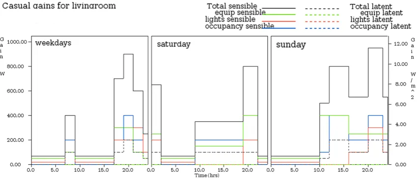
Figure 7.Building model in ESP-r: bedroom casual heat gains.

2.3.3. Materials

Seven high-performance envelopes, suitable to be used in new buildings, were investigated: two classical constructions of an externally-insulated wall and a sandwich wall and three light structures are adopted from the work of Leccese and Tuoni [17]. In addition, one ecological solution built with local materials (straw bales and earth) and a fictitious ultralight wall with EPSonly that is used as a reference. The proposed materials are intentionally all well known and commonly available in the construction market. Advanced solutions, such as phase change materials (PCM) or vacuum insulation panels (VIP), although very interesting, have not been included in this study in order to keep the attention on the design process rather than focusing on a particular technology.

The following nomenclature is used to identify the envelopes:

• A: external insulation (PTC)

• B: sandwich type (PTS)

• C: Light Wall 1 (PL1)

• D: straw bale and earth (STRB)

• E: Light Wall 2 (PL2)

• F: Light Wall 3 (PL3)

• G: EPS ultralight wall (PL4) (reference wall)

Each type is detailed in AppendixA, where the following features of each layer are specified:

• layer number

• material type

• thickness (mm)

• density (kg/m3₎

• conductivity (W/mK)

• heat capacitycp(J/kgK)

• coefficients of IR emissivityεand solar absorptionα

3. Results

3.1. Energy Analysis

The energy analysis is conducted on the basis of the methods described in Section 2.1. The following envelope indicators, illustrated in Figure8, the left part of Figure 9and in Table1, are commonly used in the design process:

• U-value (U(W/m2K))

• decrement factor (f) and time lag (τ(h))

• mass per area (Ma(kg/m2)) and static thermal capacity (Ct,a(KJ/m2K)).

The following parameters, which are observable in the right part of Figure9and also reported in Table1, are rarely adopted in practice and thus will be used in this study only for additional discussion in Section4:

• indoor admittance modulus (Yiimodulus (W/m2K)) and phase (Yiiphase (h)).

The U-value has a greater significance, for the climate of the case study, during the winter period, when the building behaviour can be reasonably approximated with a static model. The U-value is therefore the main factor used to preselect the investigated envelopes. While some of the selected seven envelopes (described in Section2) have a better U-value than others, all seven envelopes of this study allow the building to achieve a high winter performance for the considered location. The energy ranking related to the summer behaviour is then produced only in terms of the decrement factorf and the time lagτ, as per common design practice.

The comparison of the different envelope types based on decrement factor f and time lagτ indicates a five-layer light structure (label F) as the best performing (i.e., lowest decrement factor f =0.17 and large time lagτ=11 h, in Figure8) among the classic solutions, A, B, C, E, F (as listed in AppendixA) and the unconventional solution, D, which is composed of straw bales and earth, as the best overall solution (at the price of a considerable wall thickness). The envelope C and the fictitious wall G have a performance very similar to F, with a higher decrement factor (f =0.196 and f =0.200, respectively) and a higher time lag (τ≈12 h andτ≈14 h). Since the time lags are all high enough to imply an effective deferment of the diurnal outdoor temperature waves to the night, the decrement factor can be considered as more important during the ranking of these envelope types than the time lag, and therefore, F is ranked as a better solution in terms of energy. It is worthwhile to mention that G is a fictitious structure used as a reference, and therefore, the real comparison is between F and C.

Figure 9.Energy analysis.Left: mass and thermal capacity.Right: indoor admittance (mod, phase).

Table 1.Energy performance and ranking of the investigated wall types.

Wall U

f τ Ma Ct,a YiiMod Yiiph Energy

Name (W/m2K) (h) (kg/m2) (kJ/m2K) (W/m2K) (h) Ranking

A 0.320 0.200 9.67 262 223 3.54 1.92 5

B 0.318 0.321 10.14 275 234 3.89 2.20 7

C 0.121 0.196 11.93 89 133 2.01 4.33 3

D 0.126 0.063 19.55 257 249 5.49 2.14 1

E 0.124 0.205 11.31 82 101 2.60 4.02 6

F 0.274 0.171 11.10 144 127 1.44 3.47 2

G 0.062 0.200 13.77 83 90 2.36 4.37 4

3.2. Exergy Analysis

The theoretical exergy analysis illustrated in Section2.2suggests maximising the useful exergy extracted from the surrounding environment during a daily cycle in order to reduce power input requirements. In the particular case of the summer performance of a building located in a Mediterranean climate, this optimisation can be carried out by maximising the objective Function (11) over a typical summer day, in order to obtain the optimum design for the selected passive strategy (in this case, nocturnal free cooling).

The objective function suggests increasing the ventilation rate when the external temperatures are below the comfort set-point, by an amount dependent on the quality factor (exergy) of the external air. Dynamic calculations are therefore performed in free-floating mode at increasing rates of nocturnal ventilation from 0.5–10 air changes per hour (ACH). The different types of envelope sections are then quantitatively compared through the objective function (11), as reported in Figure10and Table2.

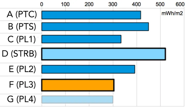
Figure 10.Objective function (10 air changes per hour (ACH), 17/08).

Table 2.Numerical values of Figure10.

Wall Name Objective Function (mWh/m2) Exergy Ranking

A 417 3

B 450 2

C 334 5

D 521 1

E 392 4

F 304 6

G 300 7

3.3. Dynamic Energy Analysis Underpinning the Exergy Calculations

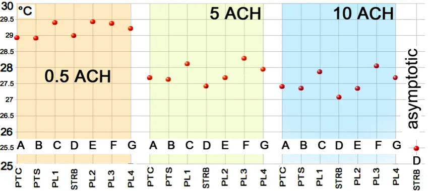
The values of maximum indoor operative temperatures, derived from the ESP-r simulations, but not directly used for ranking, are shown in Figure11and Table3. Asymptotic values are calculated, as a reference, by imposing high rates of ventilation (100 ACH; the minimum is reported in Figure11).

Table 3.Max zone operative temperature values (17 August).

Wall Type T (◦C) @ 0.5 ACH T (◦C) @ 5 ACH T (◦C) @ 10 ACH

A 28.92 27.68 27.40

B 28.91 27.63 27.35

C 29.39 28.11 27.86

D 28.99 27.42 27.07

E 29.42 27.68 27.37

F 29.37 28.28 28.05

Figure 11.Maximum zone operative Tin free-floating mode at different ACH (17 August).

4. Discussion

The energy analysis based on decrement factorf and time lagτsuggests Solutions D, F and C as the first, second and third best options for the case study. In a standard design procedure, one of these high-performance walls would be selected on the basis of other important considerations; for example, F could be chosen instead of D if the wall thickness is a concern. Solution B would be discarded because it has the worst performance in terms of decrement factor and time lag (as shown in Figure8). However, the energy performance indicators classically used in the basic design process (U-value, f andτ) do not consider the impact of internal loads, which is often relevant. More advanced energy-performance indicators, such as the thermal admittanceYii, are rarely used and are difficult to interpret. In the case study of this paper, it is actually possible to understand from the indoor admittance shown in Figure9 that Type F is characterised by a poor storage response to internal loads, since the surface flux caused by an indoor temperature variation is the lowest (≈1.5 W/m2K), as opposed to those for Envelopes D and B (≈5.5 and 4 W/m2K, respectively). However, the admittance value itself does not provide an overall quantitative ranking index for the specific case because the relative impact of the different energy indicators (U-value,f,τandYii) is not known and could not be used for suggesting possible operational strategies, such as the increase of nocturnal ventilation.

On the other hand, when considering the exergy results, the surrounding environment is analysed in search of useful interactions (second step of the design process described in Section2.2.2). The definition of the reference state as a constant value that is equal to the upper limit of comfort (26◦C in this case) implies that everything at a lower temperature is seen as a potential source of environmental “cool” exergy Benv that can contribute to indoor comfort. The simplest choice for increasing the term Benv of the exergy balance in the climate of our case study is to exploit the low temperatures of the night through nocturnal natural ventilation. We therefore carry out an investigation of different rates of night ventilation, a step that is not normally included in standard practice. The envelope reaction is explored through the objective Function (11), and the resulting exergy ranking is substantially different from the one obtained with energy considerations (apart from Envelope D), because the different construction types have different exergy storage capacities.

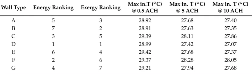
and the benefits of higher rates decrease when passing from 5 ACH–10 ACH. Asymptotic values for the best envelope option, D, show that, for the particular case study, the envelope could store enough cool exergy to maintain comfort, if enhanced exchanges with the outdoor air were implemented. The main results are summarised in Table4.

Table 4.Summary of the results.

Wall Type Energy Ranking Exergy Ranking Max in.T (

◦_{C) Max in. T (}◦_{C) Max in. T (}◦_C)

@ 0.5 ACH @ 5 ACH @10 ACH

A 5 3 28.92 27.68 27.40

B 7 2 28.91 27.63 27.35

C 3 5 29.39 28.11 27.86

D 1 1 28.99 27.42 27.07

E 6 4 29.42 27.68 27.37

F 2 6 29.37 28.28 28.05

G 4 7 29.21 27.94 27.68

5. Conclusions

This research, although very limited in scope, suggests that exergy could constitute a sound theoretical framework for a direct quantitative comparison of different storage strategies for the building envelope. Even if some conclusions can be achieved also by means of a careful analysis of the dynamic energy simulation data, especially when passive strategies are examined before the plant design, exergy considerations guide the designer directly towards the most relevant phenomena for a successful interaction with the surroundings. Therefore, properly-developed exergy indices could be a valid support in the building design process, especially where resilience and thermal autonomy represent the main targets.

In the presented case study, the exergy analysis ranking is different from the classical energy ranking adopted in the early stages of design because the investigated walls react differently to the increased ventilation rate, as some have a greater exergy storage capability than others. The nocturnal ventilation, which is selected as a simple method of exergy extraction from the environment, has a significant impact on the resultant zone temperatures and can thus be considered an effective strategy for maintaining indoor comfort when combined with a suitable envelope.

Exergy quantifies energy quality through a reference environment and thus provides an overall view and useful insight to optimise the building behaviour on a daily or seasonal basis rather than instantaneous demands. Three iterative design steps can reduce the need for a power input:

1. envelope demand reduction through energy conservation measures 2. exergy extraction from the surrounding environment

3. power input and irreversibility optimization

In the second step, the focus of this research, exergy analysis constitutes an effective guidance for investigating and enhancing useful interactions between the building and the environment.

the building and its outdoor environment and do not require more inputs than a detailed dynamic energy simulation.

Acknowledgments:The authors thank the Engineering and Physical Sciences Research Council U.K. (EPSRC, Grant No. 1586601) and the Building Research Establishment (BRE) for the financial support, as well as the anonymous reviewers for their extremely valuable contribution.

Author Contributions:Valentina Bonetti developed the study conception and design, produced the mathematical and simulation models, analysed and interpreted the results, drafted the manuscript; Georgios Kokogiannakis contributed to every stage with critical revisions.

Conflicts of Interest:The authors declare no conflict of interest. The founding sponsors had no role in the design of the study; in the collection, analyses or interpretation of data; in the writing of the manuscript; nor in the decision to publish the results.

Abbreviations

The following abbreviations are used in this manuscript:

ACH air changes per hour (1/h)

b exergy flux (W)

B exergy (J)

Ct,a static thermal capacity per area (kJ/m2K)

e energy flow (W)

E energy (J)

˙

E system energy, rate of variation (W)

f decrement factor

HVAC heating, ventilation and air-conditioning Ma mass per area (kg/m2)

PCM phase change materials ˙

Ps entropy production rate (W/K)

q heat flux (W)

Q generic heat transfer (J) q f quality factor

r entropy-energy ratio

s entropy flow (W/K)

S entropy (J/K)

˙

S system entropy, rate of variation (W/K) t time variable (s or h)

t∗ generic time (s or h)

T temperature (K)

U U-value (W/m2_K)

VIP vacuum insulation panels

Yii indoor admittance (modulus: W/m2K; phase: h)

α solar absorption coefficient

ε IR emittance coefficient

τ time lag (h)

Indexes:

air outdoor air

demand demanded by the building env surrounding environment

p power

u utility, useful effect

x generic flux

Appendix A

Details of the investigated wall constructions are reported in the tables of this section.

Table A1.Case A: externally-insulated wall, “PTC” (Layer 1 is outdoors). Thickness: 350 mm.

Layer No. Material Thickness (mm) Density Conductivity cp ε−α

(kg/m3) (W/mK) (J/kgK)

1 plaster 10 1600 1.000 880 0.91–0.26

2 exp.polystyrene 80 35 0.034 1400 0.90–0.30

3 brick 250 910 0.430 840 0.90–0.90

4 plaster 10 1600 1.000 880 0.91–0.26

Table A2.Case B: sandwich wall, “PTS” (Layer 1 is outdoors). Thickness: 340 mm.

Layer No. Material Thickness (mm) Density Conductivity cp ε−α

(kg/m3) (W/mK) (J/kgK)

1 plaster 10 1600 1.000 880 0.91–0.26

2 brick (2) 120 1000 0.400 840 0.90–0.90

3 exp. polystyrene 80 35 0.034 1400 0.90–0.30

4 brick (2) 120 1000 0.400 840 0.90–0.90

5 plaster 10 1600 1.000 880 0.91–0.26

Table A3.Case C: light wall with 8 layers, “PL1” (Layer 1 is outdoors). Thickness: 382 mm.

Layer No. Material Thickness (mm) Density Conductivity cp ε−α

(kg/m3) (W/mK) (J/kgK)

1 wood fibre 15 1400 0.200 1600 0.90–0.50

2 air gap 40 - - -

-3 OSB 20 600 0.160 1700 0.90–0.70

4 rock wool 100 80 0.035 1000 0.90–0.60

5 OSB 20 600 0.160 1700 0.90–0.70

6 exp. polystyrene 160 35 0.034 1400 0.90–0.30

7 OSB 15 600 0.160 1700 0.90–0.70

8 gypsum 12.5 1000 0.470 1000 0.91–0.22

Table A4.Case D: straw bales and earth wall, “STRB” (Layer 1 is outdoors). Thickness: 570 mm.

Layer No. Material Thickness (mm) Density Conductivity cp ε−α

(kg/m3) (W/mK) (J/kgK)

1 earth plaster 30 1400 0.600 850 0.90–0.90

2 straw 460 120 0.060 1400 0.90–0.90

Table A5.Case E: light wall with 7 layers, “PL2” (Layer 1 is outdoors). Thickness: 428 mm.

Layer No. Material Thickness (mm) Density Conductivity cp ε−α

(kg/m3) (W/mK) (J/kgK)

1 composite 30 550 0.090 1400 0.90–0.70

2 exp. polystyrene 60 35 0.034 1400 0.90–0.30

3 mineral wood 50 360 0.090 1550 0.90–0.70

4 exp. polystyrene 120 35 0.034 1400 0.90–0.30

5 rock wool 50 80 0.035 1000 0.90–0.60

6 air gap 80 - - -

-7 gypsum 37.5 1000 0.470 1000 0.91–0.22

Table A6.Case F: light wall with 5 layers, “PL3” (Layer 1 is outdoors). Thickness: 300 mm.

Layer No. Material Thickness (mm) Density Conductivity cp ε−α

(kg/m3) (W/mK) (J/kgK)

1 plaster 10 1600 0.800 1000 0.91–0.26

2 exp. polystyrene 300 35 0.034 1400 0.90–0.30

3 cellular concrete 220 500 0.130 840 0.90–0.70

4 exp. polystyrene 300 35 0.034 1400 0.90–0.30

5 plaster 10 1600 0.800 1000 0.91–0.26

Table A7.Case G: ultralight wall, “PL4” (Layer 1 is outdoors). Thickness: 580 mm.

Layer No. Material Thickness (mm) Density Conductivity cp ε−α

(kg/m3_{) (W/mK) (J/kgK)}

1 plaster 20 1600 0.800 1000 0.91–0.26

2 exp. polystyrene 540 35 0.034 1400 0.90–0.30

3 plaster 20 1600 0.800 1000 0.91–0.26

References

1. McGovern, J.A. Exergy analysis—A different perspective on energy. Part 1: The concept of exergy. Proc. Inst. Mech. Eng. Part A J. Power Energy1990,204, 253–262.

2. Bejan, A.; Vadász, P.; Kröger, D.G. Energy and the Environment; Environmental Science and Technology Library; Springer: Dordrecht, The Netherlands, 1999; Volume 15, p. 265.

3. Schmidt, D.; Torio, H.ECBCS Annex 49: Low Exergy Systems for High-Performance Buildings and Communities; Technical Report; Fraunhofer IBP: Stuttgart, Germany, 2011.

4. Pons, M. On the reference state for exergy when ambient temperature fluctuates. Int. J. Thermodyn.2009, 12, 113–121.

5. Davies, M.G. Optimum design of resistance and capacitance elements in modelling a sinusoidally excited building wall. Build. Environ.1983,18, 19–37.

6. Balaras, C.A. The role of thermal mass on the cooling load of buildings. An overview of computational methods. Energy Build.1996,24, 1–10.

7. Boji´c, M.; Loveday, D. The influence on building thermal behavior of the insulation/masonry distribution in a three-layered construction.Energy Build.1997,26, 153–157.

8. Ma, P.; Wang, L.S.; Guo, N. Energy storage and heat extraction—From thermally activated building systems (TABS) to thermally homeostatic buildings.Renew. Sustain. Energy Rev.2015,45, 677–685.

9. The ESP-rCommunity. GitHub of the ESP-r Software. Available online: https://github.com/ESP-rCommunity (accessed on 31 August 2016).

11. Torgal, F.P.; Mistretta, M.; Kaklauskas, A.; Granqvist, C.G.; Cabeza, L.F. Nearly Zero Energy Building Refurbishment. A Multidisciplinary Approach; Springer: London, UK, 2013; p. 181.

12. UNI Ente Nazionale Italiano di Unificazione. UNI/TS 11300-1; Technical Report; UNI: Milano, Italy, 2008. 13. Shukuya, M.Exergy Theory and Applications in the Built Environment; Springer: London, UK, 2013; p. 365. 14. Ursini Casalena, A. UNI EN ISO 13786 Spreadsheet, Version 2.2. Available online:

http://www.mygreenbuildings.org/2009/07/27/trasmittanza-termica-periodica-foglio-di-calcolo-excel-per-calcolare-le-proprieta-termiche-dinamiche-di-un-componente-edilizio.html (accessed on 31 August 2016). 15. Clarke, J.A.Energy Simulation in Building Design; Butterworth-Heinemann: Oxford, UK, 2001; p. 362.

16. The ESP-rCommunity. ESP-r Database. Available online: https://github.com/AGeissler/myESP-rDatabases/blo b/master/climate/ita_rome_iwec.a (accessed on 1 November 2016).

17. Leccese, F.; Tuoni, G. Pareti leggere in edilizia. Guida all’impiego secondo la piu’ recente normativa nazionale. Neo-Eubios2008,24, 14–21.

Sample Availability:Dynamic models for the ESP-r software are available from the authors.

c