VCU Scholars Compass
Theses and Dissertations Graduate School
2013
Geometric Approach to Support Vector Machines
Learning for Large Datasets
Robert Strack
Virginia Commonwealth University
Follow this and additional works at:http://scholarscompass.vcu.edu/etd Part of theComputer Sciences Commons
© The Author
This Dissertation is brought to you for free and open access by the Graduate School at VCU Scholars Compass. It has been accepted for inclusion in Theses and Dissertations by an authorized administrator of VCU Scholars Compass. For more information, please [email protected].
Downloaded from
L
L
D
A Dissertation submitted in partial fulfillment of the requirements for the degree of Doctor of Philosophy at Virginia Commonwealth University
by
RS
M.Sc. Eng., AGH University of Science and Technology (Poland), 2007
D: VOJISLAV KECMAN
ASSOCIATE PROFESSOR, DEPARTMENT OF COMPUTER SCIENCE
Virginia Commonwealth University Richmond, Virginia,
The dissertation introduces Sphere Support Vector Machines (SphereSVM) and Minimal Norm Support Vector Machines (MNSVM) as the new fast classification algorithms that use geometrical properties of the underlying classification problems to efficiently obtain models describing training data. SphereSVM is based on combining minimal enclosing ball approach, state of the art nearest point problem solvers and probabilistic techniques. The blending of the three speeds up the training phase of SVMs significantly and reaches similar (i.e., practically the same) accuracy as the other classification models over sev-eral big and large real data sets within the strict validation frame of a double (nested) cross-validation (CV). MNSVM is further simplification of SphereSVM algorithm. Here, relatively complex classification task was converted into one of the simplest geometri-cal problems – minimal norm problem. This resulted in additional speedup compared to SphereSVM. The results shown are promoting both SphereSVM and MNSVM as outstand-ing alternatives for handloutstand-ing large and ultra-large datasets in a reasonable time without switching to various parallelization schemes for SVMs algorithms proposed recently.
The variants of both algorithms, which work without explicit bias term, are also pre-sented. In addition, other techniques aiming to improve the time efficiency are discussed (such as over-relaxation and improved support vector selection scheme). Finally, the accuracy and performance of all these modifications are carefully analyzed and results based on nested cross-validation procedure are shown.
Contents
1 Introduction 2
1.1 Contributions of the Dissertation . . . 5
2 Background 6 2.1 Large Margin Classifiers . . . 6
2.1.1 L1 Support Vector Machines . . . 9
2.1.2 L2 Support Vector Machines . . . 12
2.1.3 Kernel SVM . . . 14
2.2 Fundamental Problems of the Computational Geometry . . . 16
2.2.1 Minimal Norm Problem . . . 16
2.2.1.1 Generalization to Kernel MNP . . . 18
2.2.2 Nearest Point Problem . . . 19
2.2.3 Minimal Enclosing Ball Problem . . . 20
2.2.3.1 Generalization to Kernel MEB . . . 23
2.3 Geometric L2 Support Vector Machines . . . 24
2.3.1 Nonlinear Geometric SVM . . . 28
2.3.2 L2 SVM as a Geometric Problem . . . 29
2.3.2.1 L2 SVM and Minimal Norm Problem . . . 30
2.3.2.2 L2 SVM and Minimal Enclosing Ball Problem . . . 30
2.3.3 Solving L2 SVM based on Minimal Enclosing Ball Approach . . . 31
2.3.3.1 Core Vector Machines . . . 33
2.3.3.2 Ball Vector Machines . . . 36
2.4 Geometric L1 Support Vector Machines . . . 38
2.4.1 Soft Minimal Enclosing Ball Problem . . . 38
3 Sphere Support Vector Machines 40 3.1 Relation to Ball Vector Machines . . . 40
3.2 Steps of the Algorithm . . . 41
3.2.1 Initialization . . . 41
3.2.2 Selection of Violating Vectors . . . 42
3.2.3 Update Procedure . . . 43
4 Minimal Norm Support Vector Machines 48
4.1 Relation to MEB-based algorithms . . . 48
4.2 Steps of the Algorithm . . . 49
4.2.1 Initialization . . . 49
4.2.2 Selection of the Violating Vectors . . . 50
4.2.3 Update Procedure . . . 51
4.2.4 Stopping Criterion . . . 52
4.3 Properties of the Solution and the Feature Space . . . 53
5 Implementation Techniques 56 5.1 Draw Scheme for Geometric SVM Solvers . . . 56
5.1.1 Impact on the Model Accuracy . . . 57
5.1.2 Impact on the Computational Complexity . . . 59
5.2 Multi-scale Approximation . . . 59
5.3 Over-relaxation . . . 60
5.3.1 Cycles in MDM Algorithm . . . 61
5.3.2 Successive Over-relaxation . . . 62
5.4 Alternative Approach to Multi-class Problems . . . 63
5.4.1 All-at-once SVM Training . . . 63
5.4.2 Nonlinear Multi-class Training . . . 65
5.4.3 Label Vector Selection . . . 66
5.5 Bias Evaluation . . . 66
5.5.1 Bias Evaluation in All-at-once Multi-class Training . . . 68
5.6 Other Minimal Norm Solvers in MNSVM . . . 68
5.6.1 Improved MDM . . . 69
5.6.2 Generalized IMDM . . . 70
5.6.3 MNSVM with different Minimal Norm Problem Solvers . . . 71
5.7 Model Selection based on Pattern Search . . . 71
5.7.1 Grid Search Method . . . 72
5.7.2 Pattern Search Method . . . 72
6 Role of the Bias in the Geometric Approach to SVM 76 6.1 Geometric Approach without Bias Term . . . 77
6.2 Properties of the Feature Space . . . 79
7 Experiments and Results 81 7.1 Geometric Support Vector Machines . . . 81
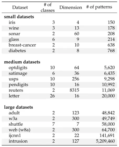
7.1.1 Datasets and Experimental Environment . . . 81
7.1.1.1 Visualization of Statistical Properties . . . 83
7.1.2 Performance of the Sphere Support Vector Machines . . . 84
7.1.2.1 Medium Datasets . . . 85
7.1.2.2 Large Datasets . . . 88
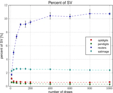
7.1.2.3 Draw Scheme for SphereSVM . . . 91
7.1.3 Performance of the Minimal Norm SVM . . . 95
7.2 Geometric SVM without Bias . . . 103
7.2.1 SphereSVM without Bias . . . 103
7.2.2 Minimal Norm SVM without Bias . . . 106
7.3 Over-relaxation . . . 108
7.3.1 Over-relaxation in SphereSVM . . . 108
7.3.2 Over-relaxation in Minimal Norm SVM . . . 111
7.4 All-at-once Approach for Multi-class Problems . . . 112
7.5 Bias Evaluation Technique . . . 116
7.6 MNSVM with Improved MDM Solver . . . 117
7.6.1 Generalized IMDM . . . 120
7.7 Sparse Grid Model Selection Technique . . . 121
7.8 GSVM toolkit . . . 123
8 Conclusions and future work 128
2.1 Common kernel types . . . 15 5.1 Estimation of the percent of violators by Agresti-Coull estimator . . . 58 7.1 Datasets used in experiments . . . 84
List of Figures
1.1 Reduced Convex Hulls . . . 4
2.1 Minimal Norm Problem. . . 17
2.2 Nearest Point Problem. . . 20
2.3 Minimal Enclosing Ball. . . 21
2.4 Hierarchy of the SVM training algorithms presented in the dissertation. . . 32
2.5 The Core Vector Machines algorithm . . . 35
2.6 The Ball Vectorm Machines algorithm . . . 38
3.1 Single iteration of the SphereSVM algorithm . . . 43
3.2 Step of the SphereSVM algorithm (convergence proof) . . . 46
4.1 Update step of the MNSVM algorithm. . . 50
4.2 Dependency betweenρand training parameters. . . 55
5.1 Estimation of the percent of violators by Agresti-Coull estimator . . . 58
5.2 Update cycle in BVM algorithm . . . 62
5.3 Pattern Search . . . 75
6.1 Support vectors in feature spaces ˜Φand ¨Φ . . . 80
7.1 Medium datasets – accuracy obtained during nested cross-validation . . . . 86
7.2 Medium datasets – total nested cross-validation time . . . 87
7.3 Medium datasets – training time for optimal parameters . . . 87
7.4 Medium datasets – average percent of support vectors . . . 88
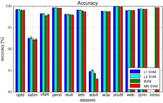
7.5 Large datasets – accuracy obtained during nested cross-validation . . . 89
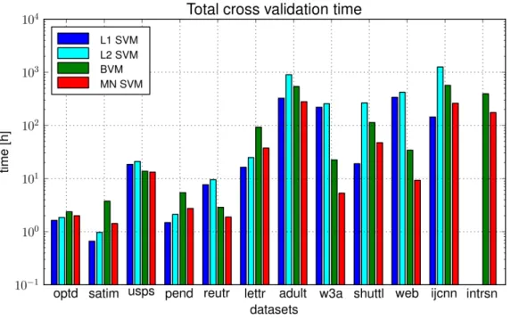
7.6 Large datasets – total nested cross-validation time . . . 90
7.7 Large datasets – training time for optimal parameters . . . 91
7.8 Large datasets – average percent of support vectors . . . 92
7.9 The training time and the number of support vectors for SphereSVM . . . . 92
7.10 Classification accuracy for different draw schemes . . . 94
7.11 Cross-validation time for different draw schemes . . . 94
7.12 Percent of support vectors for different draw schemes . . . 95
7.13 MNSVM – total nested cross validation time . . . 96
7.14 MNSVM – Training time for optimal parameters . . . 97
7.16 MNSVM – average percent of support vectors . . . 99
7.17 MNSVM training time for “checkers” data set . . . 100
7.18 Accuracy obtained by SphereSVM and MNSVM . . . 101
7.19 Cross-validation time obtained by SphereSVM and MNSVM . . . 102
7.20 Training time for optimal parameters obtained by SphereSVM and MNSVM 102 7.21 Size of the models obtained by SphereSVM and MNSVM . . . 103
7.22 Accuracy of SphereSVM without bias . . . 104
7.23 Cross-validation time for SphereSVM without bias . . . 104
7.24 Training time for SphereSVM without bias . . . 105
7.25 Percent of support vectors for SphereSVM without bias . . . 106
7.26 MNSVM without bias – accuracy . . . 107
7.27 MNSVM without bias – training time . . . 108
7.28 Accuracy of SphereSVM with over-relaxation . . . 109
7.29 Nested CV time of SphereSVM with over-relaxation . . . 110
7.30 Nested CV time of SphereSVM with over-relaxation forη≈2 . . . 110
7.31 Training time for optimal parameters for SphereSVM with OR . . . 111
7.32 Percent of support vectors for SphereSVM with over-relaxation . . . 112
7.33 Over-relaxation with MNSVM algorithm . . . 113
7.34 Total cross-validation time for all-at-once multi-class training . . . 114
7.35 Accuracy for all-at-once multi-class training . . . 115
7.36 Training time for optimal parameters for all-at-once multi-class training . . 115
7.37 Percent of support vectors for all-at-once multi-class training . . . 116
7.38 Bias evaluation – reuters . . . 117
7.39 Bias evaluation – satimage . . . 118
7.40 Training time for IMDM algorithm . . . 119
7.41 Accuracy for IMDM algorithm . . . 119
7.42 Percent of support vectors for IMDM algorithm . . . 120
7.43 MNSVM with Generalized IMDM update scheme . . . 121
7.44 Training time for Pattern Search and Grid Search methods . . . 122
7.45 Accuracy for Pattern Search and Grid Search methods . . . 122
7.46 Training time of the Pattern and Grid search methods . . . 123
7.47 Accuracy obtained by different SVM implementations . . . 125
7.48 Cross-validation time obtained by different SVM implementations . . . 125
7.49 Optimal parameters training time obtained by different SVMs . . . 126
List of Algorithms
1 Core Vector Machines Algorithm . . . 34
2 Ball Vector Machines Algorithm . . . 36
3 SphereSVM Algorithm . . . 41
4 Minimum Norm Vector Machines Algorithm . . . 49
5 Multi-scale Approximation Method . . . 60
Introduction
Support Vector Machines are known as one of the best classification tools available today. Many experimental results on variety of classification (and regression) tasks complement the highly appreciated theoretical properties of SVMs. However, there is one property of SVM’s learning algorithm which required, and it is still requiring, special attention. This is the fact that the learning phase of SVMs scales poorly with the number of training datapoints. Hence, with an increase of datasets’ sizes, the learning can be a quite slow process. The first successful attempts in resolving the issue were the chunking method described by Boser et al. [1] and the decomposition approaches introduced by Osuna et al. [2] which led to several efficient software packages the most popular being SVMlight [3] and LIBSVM [4]. However, the ever increasing size of datasets has driven the SVMs training time beyond the acceptable limits. The two remedy avenues for overcoming the issues of large datasets proposed and used in the last decade were various parallelization attempts (including the newest GPU embedded implementations [5, 6]) and the use of geometric approaches. The later includes solving SVMs’ learning problem by both convex hulls and the enclosing ball approach [7, 8]. The most recent and advanced method known as the Ball Vector Machines [9] has demonstrated high capability for handling large datasests.
The Sphere Support Vector Machine (SphereSVM) and Minimal Norm Support Vector Machines (MNSVM) proposed here combine the two techniques (namely, convex hull and enclosing balls approaches). While keeping the level of accuracy they achieve a significant speedup with respect to all three L1 and L2 LIBSVM and BVMs.
Although the most popular SVM solvers (such as Platt’s SMO [10]) are very efficient in searching for the solution in the dual space, there is a lot of research conducted towards finding efficient algorithms that work directly in the feature space. These algorithms are mostly based on the geometric interpretation of the maximum margin classifiers.
The geometric properties of the hard margin SVM classifiers have been known for a long time [11]. Recently, Keerthi et al. [12] and Franc [13] proposed algorithms based on geometric interpretation of the SVM algorithm for solving cases with separable classes. Their approach treats the problem of finding the maximum margin between two classes as a problem of finding two closest points belonging to convex polytopes covering the classes. Crisp et al. analyzed geometric properties ofν-SVM algorithm [14] and based on this work, Mavroforakis introduced the Reduced Convex Hulls (RCH) [15] (see Figure 1.1). The idea allowed using geometric approach in solving SVM problems for overlapping classes. Reduced convex hulls enabled a shrink of overlapping convex polytopes covering each class. This reduction creates the margin between two overlapping classes and allows to separate them (which was previously unfeasible with Keerthi’s and Franc’s algorithms).
Another field of research involves algorithms based on Minimal Enclosing Ball (MEB) problem. Tsang et al. [7, 16] formulated SVM problem as MEB problem and proposed Core Vector Machines (CVM) algorithm as an approach suitable for very large SVM training. Their algorithm is an application of Badoiu and Clarkson’s work [17] that investigates the use of coresets in finding approximation of MEB. This work is further generalized in [18] by allowing the use of any kernel function (and not only the normalized ones as it was previously required). Furthermore, Tsang et al. in [9] improve the idea of Core Vector
Figure 1.1: Decision boundary for a problem with two overlapping classes that was solved with reduced convex hulls. Dark blue and yellow polygons represent reduced convex hulls obtained for both classes, the black solid line is the decision boundary and the black dashed lines represent the decision margin.
Machines by introducing new algorithm not requiring QP solver – Ball Vector Machines (BVM). Additional speedup was obtained by using “probabilistic speedup” approach proposed by Smola and Sch ¨olkopf [19]. Moreover, Asharaf et al. [20] proposed another extension of CVM that is capable of handling multi-class problems.
In this dissertation we propose new algorithms that improve the BVM by applying ideas previously used in SVM learning based on RCH. SVM solver involving finding two closest points on non-overlapping RCH was introduced by Mavroforakis and Theodor-idis [15]. It was further improved by L ´opez et al. [21] by replacing SK algorithm (Kozinec [22]), that was used in searching for the closest points, with faster MDM algorithm intro-duced by Michell et al. in [23]. Our work, similarly to L ´opez’s, introduces an algorithm originated within an MDM solver as the technique for finding minimal enclosing ball. This novel MEB algorithm (SphereSVM) is successfully applied in solving MEB problem corresponding to the L2 SVM learning task. This approach is further simplified by uti-lizing connection between MEB and minimal norm problems and a new more efficient algorithm is introduced (Minimal Norm SVM).
1.1
Contributions of the Dissertation
The major contributions of the dissertation are:
• introduction of SphereSVM and MNSVM algorithms aiming to solve large
classifi-cation problems
• proof of convergence and estimation of the computational complexity of the SphereSVM
algorithm
• implementation of the over-relaxation technique in solving the Minimal Enclosing
Ball and Minimal Norm problems
• study of the role of the bias in SphereSVM and MNSVM training and introduction
of the novel version of the algorithms without bias
• application of Improved MDM solver into solving L2 SVM classification tasks based
on MNSVM algorithm
• generalization of binary (two-class) SphereSVM and MNSVM algorithms into
multi-class SVM solvers
• proposition of a new model selection approach (sparse grid search) that is capable
of finding model parameters in approximately linear time preserving the accuracy of the grid search method
• development of an efficient open-source framework called “gsvm” suitable for
Background
2.1
Large Margin Classifiers
The Generalized Portrait algorithm introduced by Vapnik [24] in mid 60’s gave a founda-tion to modern maximum margin classifiers. A theoretical basis of a principle of structural risk minimization which is the basis for developing maximal margin classifier is given in [25]. Based on the work of Aizerman [26], Boser, Guyon and Vapnik [1] generalized the original linear algorithm and applied it to a nonlinear case. Finally, the soft margin Support Vector Machines were introduced by Cortes and Vapnik [27]. This modifica-tion not only allowed to use maximum margin classifiers for non-separable datasets but also introduced the regularization parameter that can be used to prevent over-fitting the dataset.
The supervised learning is the process of determining an input-output relationship f(x) by using a training datasetX={xi}, containingminputsxifromd-dimensional input space xi ∈ Rd, and the labels yi assigned to each of these input vectors. In case of the simplest
classification problem, being called the binary classification, there are two possible output values yi ∈ {−1,1}. From now on, we assume that the datasetXis given as a matrixXof
of lengthmcontaining vector labelsyi.
The goal of binary SVM classifier is to find a classification function
f(x)=sgnd(x), (2.1) that assigns value 1 or -1 to a given vectorxdepending what is the predicted class of that vector. The functiond(x) is a linear decision function defined as
d(x)=x·w+b. (2.2)
In the case of hard margin classifiers, that do not permit classification error on the training samples, bothwand bias termbmust satisfy the following conditions
yi(xi·w+b)>1, i=1, . . . ,m. (2.3)
In addition, weight vectorwmust be of the minimal norm in order to maximize the margin between two classes. This way we minimize the chance of misclassification performed on previously unseen data samples. The width of the margin is equal to 2
kwk. Therefore,
the optimization criterion for linear hard margin SVM problem can be defined as the following quadratic optimization problem
arg min
w
kwk2, (2.4)
subject to
yi(xi·w+b)>1, i=1, . . . ,m. (2.5)
Unfortunately, this idea is not applicable to all classification problems because it does not tolerate misclassified training samples and therefore cannot be used for overlapping classes. In order to overcome this problem Cortes and Vapnik introduced soft margin
SVM [27]. The slack variablesζi represent the algebraic distance of a training data point xi from the margin. This way they made it possible to solve the SVM training problem
for overlapping classes which finally allowed to apply SVM to the broader range of classification problems.
The hard margin constrains (2.3) have been relaxed by allowing some missclassification in the following way
yi(xi·w+b)>1−ζi, i=1, . . . ,m, (2.6)
and the optimization criterion (2.4) has been changed in such way that it not only maxi-mizes the classification margin but also minimaxi-mizes the sum of distancesζiof overlapped
data points from their margins
E=
m
X
i=1
e(ζi), (2.7)
wheree(ζi) is an error function.
Finally, the soft margin SVM can be defined as follows
arg min w,ζ kwk2+C m X i=1 e(ζi), (2.8) subject to yi(xi·w+b)>1−ζi, i=1, . . . ,m. (2.9)
The parameterCis a predefined constant called penalty parameter. One may try to resolve bias-variance dilemma by proper adjustment of the value ofC. For instance, a large value of C forces a maximization of the margin and in the case of non-linear classifier may eventually lead to over-fitting and reduction of generalization capabilities of the model.
However soft margin linear SVM defined in (2.8) is still helpless when dealing with data having very complex topological structure. This problem will be addressed in further sections. Namely, nonlinear SVM will be derived by using the so-called “kernel trick”.
2.1.1
L1 Support Vector Machines
L1 SVM is a special type of soft margin SVM that has linear error functione(ζi) =ζi. The
optimization problem is defined as
arg min w,ζ kwk2+C m X i=1 ζi, (2.10) subject to yi(xi·w+b)>1−ζi, i=1, . . . ,m, (2.11a) ζi >0, i=1, . . . ,m. (2.11b)
Equation (2.10) minimizes the sum of distancesζi i.e., the classification error, and
maxi-mizes the margin between the classes. The penalty parameterCis used to find the trade offbetween these two tasks.
The constrained optimization problem (2.20) can be solved using the Lagrange multi-pliers method. The primal Lagrangian is
Lp(w,b, ζ,α,β)= 1 2kwk 2+C m X i=1 ζi − m X i=1 αi yi(xi·w+b)−1+ζi− m X i=1 βiζi, (2.12) where αi >0, i=1, . . . ,m, (2.13a) βi >0, i=1, . . . ,m, (2.13b)
are the Lagrange multipliers. The Karush-Kuhn-Tucker condition are as follows
αi yi(xi·w+b)−ρ+ζi=0, i=1, . . . ,m, (2.14a)
By equaling derivatives ofLp(w,b, ζ,α,β) with respect of w, b and ζi to 0 the following holds ∂Lp ∂w =w− m X i=1 αiyixi =0, (2.15) ∂Lp ∂b = m X i=1 αiyi =0, (2.16) ∂Lp ∂ζi = C−αi−βi =0. (2.17)
Equations (2.15) and (2.17) can be further simplified to
w= m X i=1 αiyixi, (2.18) αi+βi =C, i=1, . . . ,m. (2.19)
Finally, the dual form of (2.10) is as follows
arg min α 1 2 m X i=1 αiαjyiyj xi·xj− m X i=1 αi, (2.20) subject to 06αi 6C, i=1, . . . ,m, (2.21a) m X i=1 αiyi =0. (2.21b)
In the matrix notation, (2.20) is equivalent to
arg min
α
1 2α
where operator◦is Hadamard product (element-wise matrix multiplication).
From the KKT condition (2.14a) one can derive that
b = |1 U| X i:xi∈U yi− X j:xj∈S αjyj xi·xj , (2.23)
where S is the set of all support vectors and U ⊂ S is the set of unbounded (i.e. free)
support vectors (xi satisfying 0< αi <Candζi =0). Finally, this leads us to the following
decision function d(x)= m X i=1 αiyi(xi·x)+b. (2.24)
By replacing the scalar product from (2.20), (2.23) and (2.24) by a kernel function, being scalar product in a feature spaceΦ,
k(xi,xj)=ϕ(xi)·ϕ(xi), (2.25)
where ϕ(x) : X → Φ represents the mapping of vector xi into the feature space Φ, we
obtain nonlinear soft margin L1 SVM. Namely, the optimization criterion (2.20) becomes
arg min α 1 2 m X i=1 αiαjyiyjk(xi,xj)− m X i=1 αi, (2.26) subject to 06αi 6C, i=1, . . . ,m. (2.27)
In matrix notation (2.26) can be expressed as
arg min α 1 2α |Hα−1|α, (2.28) whereH=hyiyjk(xi,xj) i
Finally, the decision function for the L1 SVM problem becomes d(x)= m X i=1 αiyik(xi,x)+b, (2.29)
where biasbis equal to
b= |1 U| X i:xi∈U yi− X j:xj∈S αjyjk(xi,xj) . (2.30)
If the mappingϕ(x), that defines the kernel functionk(xi,xj)=ϕ(xi)·ϕ(xj), is nonlinear then
the decision function (2.29) is also nonlinear. If ϕ(x) is linear then the decision function (2.29) is equivalent to (2.24).
2.1.2
L2 Support Vector Machines
If we use error functione(ζi)=ζ2i in the definition of soft margin SVM (2.8) we obtain the
optimization problem of L2 SVM arg min w,ζ kwk2+C m X i=1 ζ2 i, (2.31) subject to yi(xi·w+b)>1−ζi, i=1, . . . ,m. (2.32)
Here, the meaning of the penalty parameterCis the same as in previously defined L1 SVM – it controls the trade offbetween the size of the margin and sum of square distances of the training data points from their corresponding margin.
The dual form of (2.31) is as follows
arg min α 1 2 m X i=1 αiαjyiyj xi·xj+ δi j C ! − m X i=1 αi, (2.33)
subject to m X i=1 αiyi =0, (2.34a) αi >0, i=1, . . . ,m, (2.34b)
where δi j is a Kronecker delta. Furthermore, the criterion (2.33) can be expressed in the
matrix notation as arg min α 1 2α |YY|◦XX|+ 1 CI α−1|α, (2.35)
whereIis the identity matrix and◦is Hadamard product (element-wise matrix product).
The decision function for L2 SVM is given in (2.2). By substitutingwwith
w= m X i=1 αiyixi, (2.36) we obtain that d(x)= m X i=1 αiyi(xi·x)+b, (2.37) where b = |1 S| m X i=1 yi− m X j=1 αjyj xi·xj + δi j C ! , (2.38) andSis the set of all support vectors.
It is possible to replace the scalar products from (2.33), (2.38) and (2.37) by a kernel function representing a scalar product in some feature spaceΦ
kxi,xj
=ϕ(xi)·ϕ(xi), (2.39)
leads to nonlinear L2 SVM where the optimization criterion (2.33) becomes arg min α 1 2 m X i=1 αiαjyiyj k xi,xj+ δi j C ! − m X i=1 αi, (2.40) subject to m X i=1 αiyi =0, (2.41a) αi >0, i=1, . . . ,m. (2.41b)
In matrix notation (2.40) can be written as
arg min α 1 2α |H+ 1 CI α−1|α, (2.42) whereH =hyiyjk xi,xj i
is the kernel matrix. The decision function for the problem (2.40) has the same structure as in L1 SVM, namely
d(x)=
m
X
i=1
αiyik(xi,x)+b, (2.43)
where biasbis again equal to
b = |1 S| m X i=1 yi− m X j=1 αjyj k xi,xj + δi j C ! , (2.44) The detailed description and extensive comparison of L1 and L2 SVM was performed by Abe in [28].
2.1.3
Kernel SVM
Two types of nonlinear SVM classifiers are presented in Sections 2.1.1 and 2.1.2. The nonlinearity was introduced by application of the so called “kernel trick”. Namely, all
Name Kernel function Properties kxi,xj = x|ixj
Linear, dot product CPD1 kxi,xj
=
x|ixj+1
d
Complete polynomial of degreed PD2 kxi,xj =e−γkxi−xjk2 Gaussian RBF PD2 kxi,xj =tanhx|i xj +b Multilayer perceptron CPD1 kxi,xj = √ 1
kxi−xjk2+β Inverse multiquadric function PD
2
Table 2.1: Most frequently used kernel types.
scalar products were replaced by a function representing dot product in a feature spaceΦ kxi,xj
=ϕ(xi)·ϕ(xi), (2.45)
whereϕ(x) : X →Φis a function mapping data points from spaceXinto the feature space
Φ.
The most popular kernel functions are presented in Table 2.1. Beside these very frequently used kernels there are more sophisticated ones e.g. kernels designed to work with graphs or images. More examples of kernel functions with explanation how to create them can be found in [29].
This dissertation exploits properties of normalized kernels i.e., kernels that fulfill the following condition
k(x,x)=τ. (2.46) The common property of such kernels is that they map all data points onto multidimen-sional sphere with center in the origin and radius
√
τ. An example of such kernel is the Gaussian kernel. Even if a kernel is not normal, it can be normalized by the following
1conditionally positive definite
operation k0xi,xj= k xi,xj q k(xi,xi)kxj,xj . (2.47)
It is obvious that kernelk0xi,xj
is normalized since it fulfills condition (2.46)
k0(x,x)=1. (2.48)
2.2
Fundamental Problems of the Computational
Geome-try
There are several Computational Geometry problems that are especially important for the SVM algorithms. The following sections describe details of Minimal Norm Problem (MNP), Nearest Point Problem (NPP) and Minimal Enclosing Ball (MEB) problem. Their relations to Support Vector Machines are shown in Section 2.3.
2.2.1
Minimal Norm Problem
The Minimal Norm Problem is a problem of finding a point c closest to the origin that belongs to the convex hull H(X) spanned by points xi ∈ X. It can be mathematically
described as
arg min
c∈H(X)
kck2, (2.49)
wherecis a point belonging to the convex hullH(X) (see Figure 2.1).
Definition The convex hull spanned by the pointsxi ∈ Xis a set of all convex combinations
of pointsxi ∈ X H(X)= m X i=1 αixi , (2.50) such thatPm
Figure 2.1: Minimal Norm Problem.
In other words, the solution of the problemc, which is a point that is closest to the origin and is enclosed by the convex hull H(X), can be expressed as a linear combination of
points defining the convex hull
c= m
X
i=1
αixi, (2.51)
whereαi are the mixing coefficients that fulfill the following conditions
αi >0, i=1, . . . ,m, (2.52) and m X i=1 αi =1. (2.53)
This allows us to reformulate the minimization criterion (2.49) as
arg min α m X i=1 m X i=j αiαj xi·xj , (2.54)
subject to m X i=1 αi =1, (2.55a) αi >0, i=1, . . . ,m. (2.55b)
Therefore, the solution of the MNP problem c = Pm
i=1αixi can be obtained by finding
mixing coefficientsαi that minimize (2.54) and satisfy (2.52) and (2.53).
The optimization task (2.54) can be expressed in the matrix notation as
arg min α α |XX|α, (2.56) subject to 1|α=1, (2.57a) αi >0, i=1, . . . ,m. (2.57b) 2.2.1.1 Generalization to Kernel MNP
The generalization of MNP problem to the kernel-MNP is straightforward. Simply, the scalar productxi·xjfrom (2.54) should be replaced by a scalar product in the feature space
Φ, defined by mappingϕ(x) :X → Φ. Then, after defining an appropriate kernel function
kxi,xj =ϕ(xi)·ϕ(xj), (2.54) can be rewritten as arg min α m X i=1 m X j=1 αiαjk xi,xj , (2.58)
subject to m X i=1 αi =1, i=1, . . . ,m, (2.59a) αi >0, i=1, . . . ,m. (2.59b)
In a matrix notation (2.58) is as follows
arg min α α |Kα, (2.60) subject to 1|α=1, (2.61a) αi >0, i=1, . . . ,m, (2.61b) whereK=hkxi,xj i
i,j is the kernel matrix.
2.2.2
Nearest Point Problem
The nearest Point Problem can be seen as a generalization of the Minimal Norm Problem. Here, instead of searching for a point of the convex hull closest to the origin, we are searching for two closest pointsc0andc00belonging to two non-overlapping convex hulls H(X0 ) andH(X00 ) arg min c0∈ H(X0 ),c00∈ H(X00 ) kc0−c00k2, (2.62)
as can be visualized in Figure 2.2. Note that forX00 = {
0}, c00 =
0and (2.62) simplifies to (2.49). Moreover, the NPP problem can be transformed to the MNP problem by using the Minkowski difference, as shown below.
Figure 2.2: Nearest Point Problem.
Definition The Minkowski difference is defined as
A B=nai−bj|a∈ A∧b∈B
o
. (2.63)
Finally, (2.62) can be rewritten as
arg min c∈H(X0 ) H(X00 ) kck2, (2.64) where c=c0 −c00. (2.65)
Since the regionH(X0) H(X00) is convex, the criterion (2.64) is equivalent to the criterion
of the minimal norm problem (2.49). Note that ifH(X0) and H(X00) are overlapping then
the NPP problem does not have a unique solution.
2.2.3
Minimal Enclosing Ball Problem
The Minimal Enclosing Ball problem is a problem of finding a smallest sphere with a centercand a radiusRthat encloses all pointsxi ∈ X(see Figure 2.3). It can be expressed
Figure 2.3: Minimal Enclosing Ball.
mathematically as the following minimization problem
arg min
R,c
R2, (2.66)
subject to
kc−xik26R2, i=1, . . . ,m. (2.67)
The optimization problem defined by (2.66) and (2.67) is a standard quadratic program-ming problem which can be solved by the Lagrange method. The primal Lagrangian is defined as Lp(c,R,α)=R2− m X i=1 αi R2− kc−xik2 (2.68) =R2− m X i=1 αi R2− kck2+2 (xi·c)− kxik2, (2.69)
whereαi are the Lagrange multipliers satisfying the following non-negativity condition:
The complementary Karush–Kuhn–Tucker conditions are defined as
αi
R2− kc−xik2=0, i=1, . . . ,m. (2.71)
By equaling the partial derivatives ofLPwith respect to the primal variablescandR, one
can obtain ∂Lp ∂R =2R−2R m X i=1 αi =0, (2.72) and ∂Lp ∂c =2 m X i=1 αic−2 m X i=1 αixi =0. (2.73) We can assume that the enclosing ball has a non-zero radius R > 0, so we can further simplify (2.72) to
m
X
i=1
αi =1, (2.74)
and using (2.74) it is possible to write (2.73) as
c= m
X
i=1
αixi. (2.75)
Moreover, from (2.71) and (2.74) it follows that the radius of the enclosing ball is equal to
R2=
m
X
i=1
αikc−xik2. (2.76)
Substituting (2.74) and (2.75) into (2.69) we obtain the dual LagrangianLd
Ld(α)=− m X i=1 m X j=1 αiαj xi·xj + m X i=1 αikxik2. (2.77)
Consequently, we can write the MEB problem as
arg min α m X i=1 m X j=1 αiαj xi ·xj− m X i=1 αikxik2, (2.78)
subject to m X i=1 αi =1, (2.79a) αi >0, i=1, . . . ,m. (2.79b)
That can be expressed in matrix notation as
arg min α α |XX|α−α|diag (XX|), (2.80) subject to 1|α=1, (2.81a) αi >0, i=1, . . . ,m, (2.81b) where diag (XX|)=k xik2
i is a vector of Euclidean norms of samplesxi.
2.2.3.1 Generalization to Kernel MEB
In order to generalize the MEB problem into the kernel-MEB problem it is necessary to replace the scalar product xi · xj by a scalar product in the feature space Φ induced by
mappingϕ(x) : X → Φ. Letkxi,xj = ϕ(xi)·ϕ(xj) be the kernel representing the scalar
product in the feature spaceΦ(X). Now, (2.78) can be written as
arg min α m X i=1 m X j=1 αiαjk xi,xj − m X i=1 αik(xi,xi), (2.82)
subject to m X i=1 αi =1, (2.83a) αi >0, i=1, . . . ,m, (2.83b)
and the radius of the enclosing ball can be evaluated as
R2 =− m X i=1 m X j=1 αiαjk xi,xj + m X i=1 αik(xi,xi). (2.84)
In the matrix notation, the criterion (2.82) is given as
arg min
α α
|Kα−diag(K)|α, (2.85)
whereK =hkxi,xj
i
i,j is the kernel matrix and diag(K)= [k(xi,xi)]i is the diagonal of the
matrixK.
Assuming that the kernelkis normalized andkxi,xj
=τis constant, the (2.82) can be further simplified to arg min α m X i=1 m X j=1 αiαjk xi,xj , (2.86)
since the term Pm
i=1αik
xi,xj
= τ is also constant and does not affect the optimization criterion. This leads to the conclusion that for normalized kernels the MEB problem is identical to the MNP problem (see the (2.58)).
2.3
Geometric L2 Support Vector Machines
In order to approach the SVM learning problem using geometric methods, Tsang et al. [7] modified the original optimization criterion for L2 SVM classifier (Section 2.3) and defined
it as a minimization of the following cost function arg min w,b,ζ,ρ 1 2kwk 2+ b2 2 −ρ+ C 2 m X i=1 ζ2 i, (2.87) subject to yi(xi·w+b)>ρ−ζi, i=1, . . . ,m. (2.88)
Compared with the original problem (2.31), the optimized function is extended with the termb22 including bias and an additional variableρ. For the L2 SVM optimization criterion, adding term b2
2 is like adding a feature having all values equal to 1 to the feature space
ϕ0 (x)= ϕ(x) 1 . (2.89)
Addingρto the cost function replaces the constraintPm
i=1αiyi =0 in the original L2 SVM
problem (2.33) withPm
i=1αi = 1. Then, the term−Pmi=1αi from the optimization criterion
(2.33) can be discarded since it is constant. Very similar modification, which adds a new variable ν into the optimization criterion, was performed by Sch ¨olkopf and Smola in their ν-SVM algorithm [30] in order to limit the number of support vectors. Here, an additional variableρ is used just to facilitate a transformation of L2 SVM into MEB and MNP problems.
Since (2.87) is a constrained optimization problem it can be solved using the Lagrange multipliers method. We form the primal Lagrangian as
Lp(w,b, ρ, ζ,α)= 1 2kwk 2+ 1 2b 2−ρ+ C 2 m X i=1 ζ2 i − m X i=1 αi yi(xi ·w+b)−ρ+ζi, (2.90) where αi >0, i=1, . . . ,m, (2.91)
and the KKT condition are as follows
αi yi(xi·w+b)−ρ+ζi=0, i=1, . . . ,m. (2.92)
Equating derivatives ofLp(w,b, ρ, ζ) with respect ofw,b,ρandζi to 0 we obtain
∂Lp ∂w =w− m X i=1 αiyixi =0, (2.93) ∂Lp ∂b =b− m X i=1 αiyi =0, (2.94) ∂Lp ∂ρ =1− m X i=1 αi =0, (2.95) and ∂Lp ∂ζi =Cζi−αi =0. (2.96)
Equations (2.93), (2.94), (2.95) and (2.96) can be further simplified to
w= m X i=1 αiyixi, (2.97) b = m X i=1 αiyi, (2.98) m X i=1 αi =1, (2.99) and ζi = αi C. (2.100)
Moreover, from (2.92) we can conclude that:
m
X
i=1
αi yi(xi·w+b)−ρ+ζi =0, (2.101)
which using (2.97), (2.98), (2.99) and (2.100) can be further simplified to
ρ =kwk2+b2+C m X i=1 ζ2 i. (2.102)
or alternatively, it can be expressed as a function in a dual-space:
ρ= m X i=1 m X j=1 αiαjyiyj xi·xj+ m X i=1 m X j=1 αiαjyiyj+ 1 C m X i=1 α2 i. (2.103)
Using Equations (2.97), (2.98) and (2.99) we rewrite Lagrange criterion (2.90) as
Ld(α)=− 1 2 m X i=1 m X j=1 αiαjyiyj xi·xj + m X i=1 m X j=1 αiαjyiyj+ 1 C m X i=1 α2 i . (2.104) This allows to rewrite the original optimization problem from (2.87) as
arg min α m X i=1 m X j=1 αiαjyiyj xi·xj + m X i=1 m X j=1 αiαjyiyj+ 1 C m X i=1 α2 i (2.105) subject to m X i=1 αi =1, (2.106a) αi >0, i=1, . . . ,m. (2.106b)
Equation (2.105), dubbed here a modified L2 SVM, can be written in a matrix notation as
arg min
α α
|(YY|◦XX|)α+α|YY|α+ 1
Cα
The decision function of the modified L2 SVM problem, defined in (2.87), is not changed
d(x)=x·w+b. (2.108)
After substitutingwfrom (2.97) andbfrom (2.98), it can be rewritten as
d(x)= m X i=1 αiyi(xi·x)+ m X i=1 αiyi. (2.109)
The decision functions of the original and the modified L2 SVM differ in expression of the bias termb(please compare (2.2) and (2.108)). The vectorwis the same for both methods.
2.3.1
Nonlinear Geometric SVM
The “kernel trick” [26] allows us to replace the scalar productxi·xjby the kernelk
xi,xj
=
ϕ(xi)·ϕ(xj) representing the scalar product in the feature space Φ defined by mapping
ϕ(x) : X →Φ. The modified L2 SVM problem (2.105) takes the form
arg min α m X i=1 m X j=1 αiαjyiyjk xi,xj + m X i=1 m X j=1 αiαjyiyj+ 1 C m X i=1 α2 i (2.110) subject to m X i=1 αi =1, (2.111a) αi >0, i=1, . . . ,m. (2.111b)
Equation (2.110) in the matrix notation is given as
arg min
α α
|Hα+α|YY|α+ 1
Cα
whereH=hyiyjk
xi,xji
i,j. The decision function (2.109) becomes
d(x)= m X i=1 αiyik(xi,x)+ m X i=1 αiyi. (2.113)
2.3.2
L2 SVM as a Geometric Problem
First, we want to introduce a new kernel ˜kxi,xjand to show that this particular kernel is a Mercer kernel. Then by using ˜kxi,xjwe show the equivalence of the modified L2 SVM problem (2.110) and two geometric tasks introduced earlier – a minimal enclosing ball problem and a minimal norm problem. In order to do that let us introduce feature space
˜
Φand the kernel function ˜kxi,xj
: X →Φ˜ that defines dot product between samplesxi
in this space ˜ kxi,xj = yiyjk xi,xj +yiyj+ δi j C, (2.114) wherekxi,xj
is the original kernel used in SVM problem andδi jis Kronecker delta. This
kernel function seamlessly encodes data labels and the original kernel kxi,xj in such way that no information about samplesxiis lost.
Ifkxi,xj
satisfies Mercer’s condition
m X i=1 m X j=1 αiαjk xi,xj >0, (2.115) than since m X i=1 m X j=1 αiαjyiyjk xi,xj >0, (2.116) m X i=1 m X j=1 αiαjyiyj >0, (2.117) and m X i=1 m X j=1 αiαj δi j C = m X i=1 α2 i C >0, (2.118)
it is true that ˜kxi,xj
also satisfies Mercer’s condition
m X i=1 m X j=1 αiαjk˜ xi,xj >0. (2.119)
2.3.2.1 L2 SVM and Minimal Norm Problem
Equation (2.114) allows to rewrite the problem (2.110) as
arg min α m X i=1 m X j=1 αiαjk˜ xi,xj , (2.120) subject to m X i=1 αi =1, (2.121a) αi >0, i=1, . . . ,m. (2.121b)
It is clear that the problem stated by the optimization criterion (2.120) is identical to the MNP problem (2.58). In other words, solutions of (2.120) which is basically a minimal norm problem in the feature ˜Φ and the extended L2 SVM problem are the same and in order to find the decision function (2.113) of the modified L2 SVM (2.110) one can resolve the optimization problem (2.120).
2.3.2.2 L2 SVM and Minimal Enclosing Ball Problem
Minimization problem (2.105) can be also treated as a MEB problem if ˜k(xi,xi) is constant
fori=1, . . . ,m. If this condition is fulfilled, then from (2.99) it follows thatPm
i=1αik˜(xi,xi)
is constant as well. In such case, it is possible to subtractPm
i=1αik˜(xi,xi) from the criterion
(2.82) which is the optimization problem for the minimal enclosing ball, namely arg min α m X i=1 m X j=1 αiαjk˜ xi,xj− m X i=1 αik˜(xi,xi), (2.122) subject to m X i=1 αi =1, (2.123a) αi >0, i=1, . . . ,m. (2.123b)
It is easy to prove that, whenk(xi,xi)=τis constant for alli=1, . . . ,m, then ˜k(xi,xi) is
also constant
˜
k(xi,xi)=τ+1+ 1
C. (2.124) This means that for all normalized kernels, such as Gaussian kernel, it is possible to treat the L2 SVM problem from (2.87) as a minimal enclosing ball problem. Finally, the solution obtained by solving MEB problem in the feature space ˜Φand the solution of the modified L2 SVM problem are equal. This means that the decision function (2.113) of the modified L2 SVM (2.110) can be found by finding the minimal enclosing ball (via solving minimization task (2.122)).
2.3.3
Solving L2 SVM based on Minimal Enclosing Ball Approach
This section shortly introduces two popular algorithms proposed by Tsang et al. and designed to solve L2 SVM as a MEB problem. These algorithms are called Core Vector Machines and Ball Vector Machines.
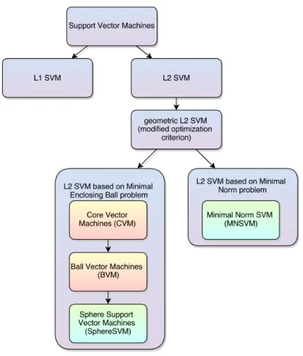
Figure 2.4 shows the hierarchy of the SVM algorithms presented in the following sections. Geometric algorithms designed by Tsang (CVM and BVM) are marked in red while methods introduced in this dissertation (SphereSVM and MNSVM) are marked in
Figure 2.4: Hierarchy of the SVM training algorithms presented in the dissertation.
green.
We use the following notation to represent vectors xi in the extended feature space ˜Φ defined by the kernel ˜kxi,xj
˜
xi =ϕ˜(xi), (2.125)
where ˜ϕis an unknown mapping function that satisfies ˜
kxi,xj
=ϕ˜(xi)·ϕ˜(xj). (2.126)
This way we can represent kernel evaluations ˜kxi,xj
as dot products ˜xi·x˜jwithout loosing
generality. Moreover, this notation conceals the complexity of the extended feature space ˜
2.3.3.1 Core Vector Machines
Tsang et al. [7] introduced an approach to SVM training called Core Vector Machines. There are two key concepts behind this algorithm. First, authors transformed the original L2-SVM problem into Minimal Enclosing Ball Problem described in section 2.2.3. Second, they applied the coreset approach [17, 31, 32, 33] in order to speedup enclosing ball calculation.
The Coreset approach The common feature of the coreset algorithms is avoidance of processing entire datasetXand focus on a smaller subset of this datasetS ⊂ Xcalled the
coreset.
Definition The coreset S(X) is a subset of the original dataset X having the following
property – the solution of some problem obtained using a coresetS⊂ Xis identical to the
solution1that would be obtained using the entire datasetX.
To illustrate the definition above, the set of support vectors is a coreset of the original datasetX, since the solution obtained by using this set would be identical to the solution
found for any other superset ofX.
The main advantage of the coreset approach is its time performance. Since|S(X)|<|X|,
the algorithm being executed for the data belonging to the coreset will yield the result faster than the algorithm using entire training dataset. Usually, in the real world applications the coreset is just a small portion of the original dataset|S(X)| |X|so the speed improvement
may be significant, especially when the computational complexity of the algorithm is large. The coreset approach was showed to be applicable for SVM training on large datasets [7, 16].
Algorithm outline The Algorithm 1 contains pseudo code of the CVM algorithm. Note that the CVM algorithm solves the modified L2 SVM problem presented in section 2.3.
Algorithm 1Core Vector Machines Algorithm
Require: ε∈[0,1){the parameter of the stopping criterion} Ensure: c=Pm
i=1αix˜i {the approximation of the MEB center}
1: S← {x˜0} 2: c ←x˜0 3: R← 0 4: while∃i:kc−x˜ik>(1+ε)Rdo 5: v←arg max ikc−x˜ik 6: S←S∪ {x˜v} 7: c,R← MEB(S) 8: end while
As it was shown earlier, the optimization problem stated in (2.87) can be transformed into corresponding MEB problem. Therefore CVM algorithm finds the L2 SVM model for (2.87) as a solution to the equivalent minimal enclosing ball problem.
The procedure starts from a small coreset S that is extended in each iteration by adding samples violating some predefined conditions. After each coreset modification new enclosing ball is calculated. A third-party QP solver can be used to solve the MEB problem – in the original CVM implementation the SMO algorithm from LIBSVM package [4] was used.
The steps of the Core Vectorm Machine algorithm are visualized on Figure 2.5.
Initialization The coreset may be initialized with a random sampleS={x˜0}as in Badoiu
and Clarkson work [34]. However, the original algorithm uses more complex initialization procedure introduced by Kumar [31] – first, a random vectorxris selected, then two vectors
are chosen ˜ xa =arg max ˜ xi kx˜r−x˜ik, (2.127) and ˜ xb=arg max ˜ xi kx˜a−x˜ik. (2.128)
Finally, the initial coreset is initialized toS={xa˜ ,xb˜ }and the radiusRis set toR= kx˜a−x˜bk 2 .
Figure 2.5: A single step of the Core Vector Machines algorithm – red points represent samples ˜xi belonging to the coreset S, solid line represents solution (minimal enclosing ball having centercand radiusR) obtained for the current core set, dashed line shows the solution that will be obtained after adding violating vector to the core set (new enclosing ball with centerc0and radiusR0
).
Finding a Violator At the beginning of each iteration a vector ˜xvbeing the worst violator
of the stopping criterion is found. Briefly speaking, it is selected by finding a vector that lays farthermost from the current centerc
xv =arg max
˜
xi∈X˜
kc−x˜ik. (2.129)
The algorithm continues until there are no vectors being farther than (1 +ε)R from the center of the minimal enclosing ball surrounding core vectors. εis a parameter of the algorithm. The smaller εis, the more accurate the solution is (but the time required for finding MEB increases as well). After the algorithm stops, all data points are within the ball with centercand radius (1+ε)R– this ball is calledε-approximation of the minimal enclosing ball.
Update step In each iteration, after the violator ˜xv is found, the entire weight vectorα is recalculated and the new centerc0
of the minimal enclosing ball, surrounding vectors ˜
Properties of the Coreset An important property of this algorithm is that the enclosing ball is spanned only by the elements from the coreset and all the vectors belonging to the coreset become the support vectors. Moreover, the following condition holds – ifαi > 0
then ˜xi ∈ S. It is possible thatScontains a vector ˜xi corresponding toαi = 0. Such vector
could have been inserted into the coreset at some point of the procedure execution but it does not participate in forming of the minimal enclosing ball. This is actually one of the drawbacks of the CVM algorithm because the coreset is not optimal. Namely, it is possible that there exists a smaller setS0 ⊂
Sthat corresponds to the same solution.
Convergence It was shown in [7] that CVM algorithm converges after at most2εiterations and that its computational complexity toOεm2 +ε14
. If the probabilistic speedup technique [34] is used then the time complexity is equal to Oε18
and it is not dependent upon the size of the datasetm.
2.3.3.2 Ball Vector Machines
Tsang et al. [9] improved Core Vector Machines by replacing the complex QP solver, used in minimal enclosing ball calculation, by much simpler iterative algorithm. In each iteration, instead of launching QP solver, only one update to the ball center is performed.
Algorithm 2Ball Vector Machines Algorithm
Require: ε∈[0,1){the parameter of the stopping criterion} Ensure: c=Pm
i=1αix˜i {the approximation of the MEB center}
1: α← 0, α0← 1 2: Rˆ ← q τ+1+ C1 3: while∃i:kc−x˜ik>(1+ε) ˆRdo 4: v←arg max ikc−x˜ik 5: β←1− R kc−xvk 6: α←(1−β)α 7: αv← αv+β 8: end while
Algorithm outline A simplified pseudo code of the algorithm is presented in Algorithm 2 (this listing does not contain probabilistic speedup [34] and multi-scale enclosing ball approximation techniques [9]).
Initialization First, the vectorαrepresenting the center of the ball from (2.75) is initial-ized such that allαi coefficients are equal to 0 except for a randomly chosen one, whose
value is set to 1 (see the initialization procedure for the CVM algorithm). For simplicity, in Algorithm 2, vector ˜x0was chosen to initialize the coreset and its weightα0was set to 1.
The radius ˆRof the enclosing ball is estimated as
ˆ R=
r
τ+1+ 1
C, (2.130)
whereτ=k(xi,xi) is the square norm in the original feature spaceΦ. The estimated radius
ˆ
Ris in fact an upper bound of the true radius. Fortunately, this estimation is very accurate when either the number of data is large or the feature space is highly dimensional.
Finding a Violator In each iteration, a point ˜xv, called violating vector and being located
outside of the enclosing ball, is selected. The algorithm continues until requirements of the stopping criterion are met (i.e. it is not possible to find a vector located outside of the ball).
Update step The centercis shifted towards the violator ˜xvin such a way that the violating
point is laying on the surface of the new ball and the following equation holds
kc0−x˜vk=R. (2.131)
The update of the center of the ball is performed along the line connecting the center c
and the violator ˜xv
Figure 2.6: A single step of the Ball Vector Machines algorithm – red points represent samples ˜xi belonging to the core setS, solid line represents current solution (the minimal enclosing ball), dashed line shows the solution that will be obtained after shifting the current solution towards the violator.
whereβis equal to
β=1− R
kc−x˜vk. (2.133)
The visualization of the algorithm’s steps is shown in Figure 2.6.
Convergence It was proved in [9] that the BVM algorithm terminates in at most ε12
iterations and its computational complexity is Oε14
. Similarly as in the case of CVM algorithm, probabilistic speedup technique made the complexity independent of the size of the datasetm.
2.4
Geometric L1 Support Vector Machines
2.4.1
Soft Minimal Enclosing Ball Problem
Let us define the soft-MEB problem as a minimization of
arg min R,c,d R2+ 1 mν m X i=1 d2i, (2.134)
subject to
kc−xik2 6R2+d2
i, (2.135)
for alli=1, . . . ,m. Namely, we try to minimize the radius of the enclosing ball simultane-ously allowing some violators.
It can be proved that the solution of the above problem is equivalent to the solution of the following modifiedν-SVM problem
arg min w,b,ζ,ρ 1 2kwk 2+b2 2 − ρ mν + C 2 m X i=1 ζi, (2.136) subject to yi(xi·w+b)>ρ−ζi, (2.137)
for alli =1, . . . ,m. Unfortunately, no efficient algorithm capable of solving the soft-MEB problem is known at this point.
Sphere Support Vector Machines
3.1
Relation to Ball Vector Machines
The SphereSVM algorithm, proposed in this work, is a novel reforumlation of the BVM approach. Therefore, some parts of both algorithms are similar. For instance, the ini-tialization procedure, the way the violating vectors are found and the stopping criterion are the same. However, there are important differences, the main one being the way how the updates of the center are performed. Unlike in BVM, the focus of SphereSVM is directed towards elimination of support vectors being inside of the enclosing ball rather than finding outlying data samples. This approach leads to fulfillment of the KKT condi-tions and therefore is a correct approach in obtaining correct solution. It applies the ideas introduced in the MDM algorithm, by Michel et al. [23], as a solution to Nearest Point Problem (NPP). Here, we adopted the MDM approach into solving the MEB problem.
The simplified pseudo code of the SphereSVM algorithm is presented in the Algorithm 3. There are two main differences between the pseudo code we present and the actual implementation that was used in our experiments. First, we used kernel cache in order not to repeat unnecessary kernel computations. Second, our implementation contains additional step tuning the values of α vector (in each iteration another update to the
Algorithm 3SphereSVM Algorithm
Require: ε∈[0,1){the parameter of the stopping criterion} Ensure: c=Pm
i=1αix˜i {the approximation of the MEB center}
1: α← 0, α0← 1 2: Rˆ ← q τ+1+ C1 3: while∃i:kc−x˜ik>(1+ε) ˆRdo 4: v←arg maxikc−xi˜k 5: u←arg min i:αi>0 kc−x˜ik 6: ρ= (˜xvk−x˜x˜u)·(˜xv−c) v−x˜uk2 7: βˆ←ρ− q ρ2− kx˜v−ck2−Rˆ2 kx˜v−x˜uk2 8: β←minnβ, αˆ u o 9: αv← αv+β 10: αu←αu−β 11: end while
vectorαis performed with such difference that the violator ˜xvis searched among support
vectors only).
3.2
Steps of the Algorithm
3.2.1
Initialization
During the initialization part of the algorithm (lines 1 to 2) a random support vector is chosen (here, the support vector with index 0) and its weight is initialized to 1. Then, the radius of the enclosing ball is estimated as
ˆ R=
r
τ+1+ 1
C, (3.1)
whereτ =k(xi,xi) is the square norm of the vectorsxi in the feature spaceΦinducted by
kernelkxi,xj
. The algorithm requires that the kernelkxi,xj
is normalized and maps all data pointsxi onto a sphere (having radius
√
τ).
dimen-sionality of the feature space are large then the difference betweenRand ˆRis negligible.
3.2.2
Selection of Violating Vectors
In the case of the BVM algorithm all weightsαi corresponding to vectors ˜xi belonging to
the coreset are modified in each updating step. SphereSVM algorithm, proposed here, updates only two weightsαvandαu. The first weightαvcorresponds to the vector that is
farthermost from the ball center while the other weightαubelongs to the support vector
closest to the center. According to the following KKT conditions of the MEB problem
αi
kc−x˜ik2−R2=0, (3.2)
if the conditionαi , 0 holds then ˜xi lies on the boundary of the minimal enclosing ball.
In other words, the vectors inside the ball are not support vectors and do not affect the solution. This observation leads to the conclusion that there are two types of violators – the vectors laying outside of the enclosing ball and the vectors with nonzero weights inside the ball. The SphereSVM algorithm aims at eliminating support vectors from inside the ball.
Similarly as in MDM algorithm, in each iteration two violating vectors are selected. First, a vector ˜xv, whose distance from the center of the ball cis greater than (1+ε) ˆR, is
chosen. If no outlier satisfying conditionkc−xi˜k >(1+ε) ˆRis found, then the algorithm
stops. Finally, after violator ˜xv is selected, searching for another violator begins. The algorithm finds a support vector ˜xu that violates the KKT conditions (3.2) the most. In
other words, the algorithm is searching for a vector ˜xuthat satisfiesαu >0 and lies closest
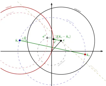
Figure 3.1: One step of the SphereSVM algorithm. The centercis being shifted parallel to the vector ˜xv−x˜uto the new positionc0. After that, vector ˜xvbecomes the support vector.
Previously estimated radius ˆRof the enclosing ball does not change.
3.2.3
Update Procedure
After the two violating vectors are selected, an update to the center of the ball is performed. Briefly speaking, the center of the ball is shifted parallel to the line connecting the two violating vectors
c0 =c+β(˜xv−x˜u), (3.3)
as shown in Figure 3.1.
The coefficientβis selected in such a way that the new sphere centered atc0is touching the violator ˜xv(˜xvmust be laying on the boundary of the new enclosing ball). Specifically,
the following condition is to be satisfied
kc0−x˜vk=R.ˆ (3.4)
Substituting (3.3) into (3.4) we obtain that
which can be reduced to the following ˆ β=ρ− s ρ2− kx˜v−ck 2−Rˆ2 kxv˜ −xu˜ k2 , (3.6) whereρis ρ= (˜xv−x˜u)·(˜xv−c) kx˜v−x˜uk2 . (3.7) In the dual space, (3.3) is equivalent to the increase of αv byβ and the decrease ofαu
also byβ(lines 9 and 10 of Algorithm 3). It is important to keep all the conditions arising from the Lagrange multiplier method satisfied. In particular, the non-negativity condition of theαi weights must be fulfilled. Therefore,β 6 1−αvand β6 αumust hold. The first
of these requirements is always fulfilled. However, one must assure non-negativity of all αi. For this reasonβcoefficient must be limited from above by the weightαu
β=minnβ, αˆ u
o
. (3.8)
Having the valueβ, it is possible to update the center of the ball and resume the algorithm by checking the stopping criterion and by searching for other violators.
3.3
Convergence and Computational Complexity
The goal of SphereSVM is to obtain aε-approximation of the MEB that satisfieskc−x˜ik6
(1+ε) ˆRfor all vectors ˜xi.
From the KKT conditions (3.2), we know that forα, being the solution of the problem stated in (2.66) and (2.67), the following inequality holds
m
X
i=1
Moreover, this property holds for all possible vectorsαhavingαi >0 and Pm i=1αi =1 m X i=1 αikc−xi˜ k2 =Rˆ2− kck26Rˆ2. (3.10)
The initialization procedure of the algorithm ensures that Pm
i=1αikc −x˜ik2 = 0. In each
iteration, the center update expressed in (3.3) changes the value ofPm
i=1αikc−x˜ik2by m X i=1 α0 ikc 0− ˜ xik2− m X i=1 αikc−xi˜ k2 =−2β(˜xv−xu˜ )·c−β2kxv˜ −xu˜ k2. (3.11)
Now, in order to prove the convergence of the algorithm, it is sufficient to show that this change increases the sumPm
i=1αikc−x˜ik2by a value greater than some positive constant.
Let us assume that the ratio of the number of updates where ˆβ > αu(clipped updates)
to the number of updates havingβ =minnβ, αˆ u
o
=βˆ(full updates) is limited by a constant. In other words, we postulate that the number of clipped updates (updates limited by the value of weight αu) is not significantly larger than the number of full updates. This
hypothesis is more than feasible. The results presented in figures 7.4 and 7.8 reveal that the numbers of support vectors for BVM algorithm, which is not capable of removing support vectors from the coreset, and SphereSVM method, which can discard support vectors from the coreset (by performing clipped update), are similar. This allows us to conclude that the vectors once selected to become support vectors are very unlikely to be eliminated from the final coreset. Therefore, the number of clipped updates is expected to be much smaller than the number of full updates (the experiments revealed that the number of clipped updates is usually much less than 1% of all updates). For this reason, we can analyze only the updates for which β = βˆ and assume that all other updates do not increase the value ofPm
i=1αikc−x˜ik2at all.
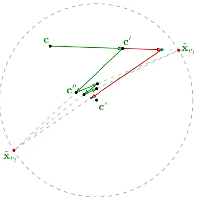
Figure 3.2 visualizes the update step performed by the SphereSVM algorithm. It contains the projection of the feature space ˜Φonto the plane determined by the violators ˜
Figure 3.2: Visualization of the update step (projection on the plane determined by points ˜
xv, ˜xuand the ball centerc) – black circle is the current solution, which is a ball with center <