Modelling stochastic bivariate mortality

City, University of London Institutional Repository

Citation

: Luciano, E., Spreeuw, J. and Vigna, E. (2006). Modelling stochastic bivariate

mortality (Actuarial Research Paper No. 170). London, UK: Faculty of Actuarial Science &

Insurance, City University London.

This is the unspecified version of the paper.

This version of the publication may differ from the final published

version.

Permanent repository link:

http://openaccess.city.ac.uk/2302/

Link to published version

: Actuarial Research Paper No. 170

Copyright and reuse:

City Research Online aims to make research

outputs of City, University of London available to a wider audience.

Copyright and Moral Rights remain with the author(s) and/or copyright

holders. URLs from City Research Online may be freely distributed and

linked to.

City Research Online: http://openaccess.city.ac.uk/ [email protected]

Faculty of Actuarial

Science

and

Insurance

Modelling Stochastic Bivariate

Mortality

Elisa Luciano, Jaap Spreeuw and

Elena Vigna

Actuarial Research Paper

No. 170

April 2006

ISBN 1 901615-97-9

Cass Business School

106

Bunhill

Row

London

EC1Y

8TZ

T +44 (0)20 7040 8470

www.cass.city.ac.uk

Modelling stochastic bivariate mortality

Elisa Luciano , Jaap Spreeuw

_{and Elena Vigna}

*University of Turin, Icer and Fondazione Collegio Carlo Alberto, Turin

+ Cass Business School, London

** University of Turin

August 5, 2006

Abstract

Stochastic mortality, i.e. modelling death arrival via a jump process with stochastic intensity, is gaining increasing reputation as a way to rep-resent mortality risk. This paper reprep-resents a …rst attempt to model the mortality risk of couples of individuals, according to the stochastic inten-sity approach.

On the theoretical side, we extend to couples the Cox processes set up, i.e. the idea that mortality is driven by a jump process whose intensity is itself a stochastic process, proper of a particular generation within each gender. Dependence between the survival times of the members of a cou-ple is captured by an Archimedean copula.

On the calibration side, we …t the joint survival function by calibrating separately the (analytical) copula and the (analytical) margins. First, we select the best …t copula according to the methodology of Wang and Wells (2000) for censored data. Then, we provide a sample-based calibration for the intensity, using a time-homogeneous, non mean-reverting, a¢ ne process: this gives the analytical marginal survival functions. Coupling the best …t copula with the calibrated margins we obtain, on a sample generation, a joint survival function which incorporates the stochastic na-ture of mortality improvements and is far from representing independency. On the contrary, since the best …t copula turns out to be a Nelsen one, dependency is increasing with age and long-term dependence exists.

Keywords: stochastic mortality, joint survival functions, copula func-tions, model selection

Acknowledgement 1 The authors wish to acknowledge the Society of Actuaries, through the courtesy of Edward (Jed) Frees and Emiliano Valdez, for providing the data used in this paper.

1

Introduction

Longevity risk, that is the tendency of individuals to live longer and longer, has been increasingly attracting the attention of the actuarial literature. More generally, mortality risk, that is the occurrence of unexpected changes in sur-vivorship, is a well accepted phenomenon.

One way to incorporate improvements in survivorship, especially at old ages, is to introduce the so called stochastic mortality. Formally, this boils down to describing death arrival as a doubly stochastic or Cox process. Intuitively, it consists in interpreting death arrival as the …rst jump time of a Poisson-like process, whose intensity, contrary to the one of the standard Poisson, is a stochastic process. A priori then two sources of uncertainty impinge on each individual: a common one, represented by the intensity, and an idiosyncratic one, represented by the actual jump time, for a given intensity. Mortality risk is captured by the behavior of the common risk factor, the intensity. The term “common” extends here to a whole generation within a gender.

The stochastic mortality approach has been proposed by Milevsky and Promis-low (2001) and developed by Dahl (2004), Cairns et al. (2005), Bi¢ s (2005), Schrager (2005), Luciano and Vigna (2005). The probabilistic setting however can be traced back to Brémaud (1981), and has been quite extensively applied in the …nancial literature on default arrival (see for instance the seminal works of Artzner and Delbaen (1992), Du¢ e and Singleton (1999) and Lando (1998)). Provided that univariate a¢ ne processes are used for the intensity, the approach leads to analytical representations of survival probabilities.

Up to now, no attempt has been made to model stochastically, in the sense just speci…ed, the survivorship of couples of individuals. This paper attempts to …ll up this gap, making use of the copula approach. Therefore, we model and calibrate separately the marginal survival functions and the copula, which, as is well known, permits to obtain the joint survival function from the marginal ones.

We work with analytical marginal survival functions as well as analytic cop-ulas, so that we end up with a fully parametric speci…cation of the joint survival function of the population, which can be extended to durations longer than the observation period.

We apply our modelling and calibration procedure to a huge sample of joint survival data, belonging to a Canadian insurer, which has been used in order to discuss (non stochastic) joint mortality in Frees et al. (1996), Carriere (2000), Shemyakin and Youn (2001) and Youn and Shemyakin (1999, 2001).

case with censoring the approach of Genest and Rivest (1993), has the advan-tage of allowing not only the calibration of the parameters for each Archimedean copula, but also of suggesting which is "the best …t" Archimedean copula in the calibrated group.

From Section 5 onwards we apply the theoretical framework and the calibra-tion method to the data sample: we present the data set, we …nd the empirical margins with the Kaplan-Meier methodology, we apply the Wang and Wells’ copula calibration procedure, and compare its results with the ones of the om-nibus procedure. We then derive the marginal survival functions, adapting the procedure in Luciano and Vigna (2005). In Section 6 the speci…c "best …t" copula obtained, together with the analytical margins, permits us to present an estimate of the joint survival function and to discuss the measures of time-dependent association, following the results in Spreeuw (2006). Section 7 con-cludes.

2

Modelling bivariate survival functions with

cop-ulas

Suppose that the heads (x) and (y); belonging respectively tom the gender

m(males) and f (females), have remaining lifetimesT_xm and T_yf, respectively, both with continuous distributions. We denote the marginal survival functions by Sxm and Syf, respectively, so that, for all t 0, Sxm(t) = Pr [Txm> t] and

Sf

y(t) = Pr Tyf > t . By Sklar’s theorem, there exists a unique copula, denoted

byC, such that for all(s; t)₂R2_{the joint survival function, denoted byS, can}

be represented as:

S(s; t) =C(S_xm(s); Sf_y(t)):

The copula approach has become a popular method of modelling the (non sto-chastic) bivariate survival function of the two lives of one couple. Both Frees et al. (1996) and Carriere (2000) present fully parametric models, using maximum likelihood, where the marginal distribution functions (Frees et al.) or survival functions (Carriere) are assumed to be of Gompertz type. Frees et al. (1996) use Frank’s copula, with a single parameter of dependence, and couple the two lives from the time of birth. Carriere (2000) on the other hand, discusses several copulas with more than one parameter (Frank, Clayton, Normal, Linear Mixing, Correlated Frailty), and couples the lives at the start of the observation period. Using the same data set, in an attempt to address the issue of di¤erent types of dependence, Youn and Shemyakin (1999, 2001) re…ne Frees et al.’s method by classifying individuals according to the age di¤erence between the female and the male member of each couple. Shemyakin and Youn (2001) adopt a Bayesian methodology as an alternative. All three papers use the Gumbel-Hougaard copula.

margins lead to di¤erent estimates of copula parameters, and may even lead to di¤erent choices of the type of copula itself. Since di¤erent copulas entail di¤erent characteristics regarding the type of dependence and aging properties, as shown in Spreeuw (2006), the choice of the right copula is essential.

Ideally, the process of choosing a copula should be completely independent of the speci…cation of the margins. Genest and Rivest (1993) have shown that this is feasible for Archimedean copulas, as long as data are complete, i.e. un-censored. Denuit et al. (2001) managed to get hold of complete data by visiting cemeteries. Applying the method developed by Genest and Rivest (1993), they established a weak correlation of lifetimes between males and females, and iden-ti…ed several plausible candidates for the copula.

Genest and Rivest’s method cannot be used if data are censored. This is the case for the data set from the large Canadian insurer as described in Section 5. The period of observation is slightly longer than …ve years, and most lives were still alive at the end of the period of observation.

Wang and Wells (2000) have extended Genest and Rivest’s method to bivari-ate right-censored data. Their methodology has been applied to Loss-ALAE data by Denuit et al. (2004). The procedure requires a nonparametric estimator of the joint bivariate survival function. A popular candidate of such an estima-tor is Dabrowska (1988), which needs estimates of the margins in accordance with Kaplan-Meier.

Following Denuit et al. (2004), we are going to apply the Wang and Wells’ method for the data set. This is a methodology which allows at the same time the calibration of the copula parameters - for any given copula family in the Archimedean class –and the choice of the best …t copula among the calibrated ones.

This paper di¤ers from the aforementioned papers on bivariate survival mod-els (Frees et al., 1996, Carriere, 2000, Shemyakin and Youn, 2001, Youn and Shemyakin, 1999, 2001, Denuit et al., 2001) not only because we include sto-chastic mortality improvements at the marginal level, but also because, instead of assuming a speci…c copula, we select a best …tting one by following the Genest and Rivest/Wang and Wells procedure for censored data. Using Wang and Wells means that we maintain the Archimedean assumption for the cop-ula. Archimedean copulas have been widely used, due to their mathematical tractability. The Archimedean class is rich, so allowing for Archimedean copulas only does not seem to be very restrictive. We refer the reader to the book by Nelsen (1999) for a review of Archimedean copulas’ de…nition and properties, and to Cherubini et al. (2004) for their applications.

In the Archimedean class in particular we will take into consideration the copulas in Table 1.

We have selected these families following the results in Spreeuw (2006), who studied the type of time-dependent association implied by many Archimedean copulas.

No. Name Generator C(u; v) Kendall’s

(t)

1 Clayton t 1 u +v 1

1

+2

2 Gumbel- ( lnt) exp ( lnu) + ( lnv)

1

1 1

Hougaard

3 Frank lne_e t ₁1 1ln 1 + (e

u

1)(e v 1)

e 1 1

4 R

t=0

t

(et ₁₎dt 1

4 Nelsen exp t e ln exp u + exp v e

1

1 4 ₊₂1

R1

t=0t +1exp 1 t

5 Special _t1 t 2 1 W+p4 +W2 _{; Complicated form}

W = (u) + (u) Table 1: Archimedean copula families

First of all, we have the rescaled conditional probability, denoted by ₁(s; t):

1(s; t) =

Pr Tm

x > s Tyf> t

Pr [Tm x > s]

= S(s; t)

Sm x (s)S

f y(t)

= Pr T

f

y > tjTxm> s

PrhTyf > t

i ; (1)

for …xed t and s. This measure has an interpretation in terms of conditional probabilities. IfTm

x andTyf are independent, then 1(s; t) = 1for alls 0and

t 0. IfTm

x andTyf are positively associated, then 1(s; t)>1 for all s >0

andt >0, with ₁ monotone nondecreasing in each argument.

Secondly Anderson et al. (1992) discuss the conditional expected residual lifetimes of(x)and(y)which we will specify as _2x(s; t)and _2y(s; t), respec-tively

2x(s; t) =

E Tm

x s Txm> s; Tyf > t

E[Tm

x sjTxm> s]

2y(s; t) =

E Tf

y t Txm> s; Tyf > t

EhTyf t Tyf > t

i : (2)

The measure _2x(s; t) ( _2y(s; t)) describes how the knowledge that Tf y > t

(Tm

x > s) a¤ects the expected lifetime of Txm (Tyf). Independence of Txm and

Tf

y implies 2x(s; t) = 2y(s; t) = 1, while if Txm and Tyf are positively

as-sociated, then _2x(s; t) > 1 and _2y(s; t) > 1 for all s > 0 and t > 0, with

2x(s; t)( 2y(s; t)) monotone nondecreasing int (s). We will concentrate on

The third measure is the cross-ratio functionCR(S(tt; t2)), de…ned in

Clay-ton (1978) and Oakes (1989) as

CR(S(s; t)) = S(s; t)

d ds

d dtS(s; t) d

dsS(s; t) d dtS(s; t)

:

Spreeuw (2006) has shown that for Archimedean copulas and u=s =t, this de…nition reduces to an expression in terms of the inverse of the generator as

CR(S(u; u)) =

0 B @

1_(v) 1 00_(v) 1 0_(v) 2

1 C A

v= (S(u;u))

: (3)

Oakes (1994) derived a similar expression for frailty models (being a subclass of Archimedean copula models).

The cross-ratio function speci…es the relative increase of the force of mor-tality of the survivor, immediately upon death of the partner. IfCR(S(u; u)) increases (decreases) as a function of u, this means that members of a cou-ple become more (less) dependent on each other as they age. Manatunga and Oakes (1996) have demonstrated that a plot ofCR(v)versus1 v, forv₂[0;1] can be used as a diagnostic technique for assessing goodness of …t. (Note that

S(0;0) = 1andlimu!1S(u; u) = 0.)

The …rst copula in Table 1, Clayton, will be studied because it is well known and bears the special property of the association remaining constant over time. Copulas2(Gumbel-Hougaard) and3 (Frank) share the characteristics of being well known as well. Moreover, unlike Clayton, the association is decreasing over time. Copula families4 and5 are due to Nelsen (1999). Family4 can be identi…ed as “Family4:2:20” in Chapter 4 of Nelsen (1999) and will henceforth be referred to as the “Nelsen copula”. It is studied, since, unlike the …rst three copulas, the association is increasing over time. And …nally copula5, which is also due to Chapter 4 of Nelsen (1999), will be labelled as the “Special copula”. It di¤ers from the other four, in the sense that the dependence between the two risks is not necessarily of a long-term type. Like the Nelsen copula, association is increasing in time.

3

Marginal stochastic mortality

the doubly stochastic approach to mortality modelling. Then we summarize some previous …ndings, which justify the modelling choice for the intensity made in this paper.

3.1

Theoretical framework

3.1.1 Cox processes

Following Lando (1998, 2004), let us assume a complete probability space( ;_F;P);

a processXtofRd-valued state variables (t T) and the …ltrationfGt:t 0g

of sub- -algebras of_F generated by X;i.e. _Gt= fXs; 0 s tg, satisfying

the usual conditions.

Let be a nonnegative measurable function s.t. R₀t (Xs)ds < 1 almost

surely and de…ne the …rst jump time of a nonexplosive adapted counting process

Ntas follows:

= inf t:

Z t

0

(Xs)ds E1 (4)

whereE1 is an exponential random variable with unit parameter. In addition,

let us consider the enlarged …ltration_Ft, generated by both the state variable

and the jump processes:

Ft = Gt_ Ht;

Ht = fNs; 0 s tg

and assume that the_H0 …ltration is trivial, in that no jump occurs at time 0:

Under this construction, the processNtis said to admit the intensity (Xs), if

the compensator ofNtadmits the representation R₀t (Xs)ds, i.e. if

Mt=Nt

Z t

0

(Xs)ds

is a local martingale. If the stronger conditionE R0t (Xs)ds <1is satis…ed,

Mt=Nt R₀t (Xs)dsis a martingale.

Intuitively, this implies that, given the history of the state variables up to time

t, the counting process is "locally" an inhomogeneous Poisson process, which jumps according to the intensity (Xt):

E(Nt+ t NtjGt) = (Xt) t+o( t):

Formally, the construction (4) easily implies that the survival function of the …rst jump time , evaluated at time 0, and conditional on knowledge of the state process up to timet, is

Pr( > t_jGt) = exp

Z t

0

wherePr(:)is the probability associated to the measureP. It can also be shown, by simple conditioning, that the time 0 unconditional survival probability, which we will denote asS(t), is

S(t) = Pr( > t) =E exp

Z t

0

(Xs)ds : (5)

The unconditional probability at any datet0 _{greater than 0 can be shown to be}

Pr( > t_{j F}t0) =I_{f >t}0_gE exp

Z t t0

(Xs)ds j Gt0

whereIf >t0_g is the indicator function of the event > t0.

A nonexplosive counting processNtconstructed as above is said to be aCox

ordoubly stochastic process driven by_fGt:t 0g. The corresponding …rst jump

time isdoubly stochastic with intensity (Xs).

As a particular case, any Poisson process is a doubly stochastic process driven by the …ltration_Gt= (;; ) =G0 for anyt 0, in that the intensity is

deter-ministic.

These results can be naturally applied in the actuarial domain: if is the future lifetime of a head agedx,Tx, his/her survival function,Sx(t), is

Sx(t) = Pr(Tx> t) =E exp

Z t

0

(Xs)ds (6)

3.1.2 A¢ ne processes

In general, the expectations (5) and (6) are not known in closed form: however, a remarkable exception is the case in which the dynamics ofX is given by the SDE:

dX(t) =f(X(t))dt+g(X(t))dW~(t) +dJ(t);

whereW~ is an n-dimensional Brownian motion,J is a pure jump process, and, above, all the driftf(X(t)), the covariance matrixg(X(t))g(X(t))0_{and the jump}

measure associated withJ have a¢ ne dependence on X(t). Such a process is named an a¢ ne process, and a thorough treatment of these processes is in Du¢ e et al. (2003).

The convenience of adopting a¢ ne processes in modelling the intensity lies in the fact that, under technical conditions, it yields:

Sx(t) =E

h

eR0t (X(s))ds

i

3.2

Selection of the intensity

In the existing actuarial literature, di¤erent classes of a¢ ne processes have been chosen for the intensity of mortality. For example, Milevsky and Promislow (2001) investigate a so-called mean reverting Brownian Gompertz speci…cation, with intensityht given by

ht=h0e

gt+ R₀te b(t u)dW h_u

t ;

withg; ; bconstant and the Brownian motionW uni-dimensional.

Dahl (2004) selects an extended Cox-Ingersoll-Ross (CIR) process, i.e. a time-inhomogeneous process , reverting to a deterministic function of time

d _x+t= ( (t; x) (t; x) _x+t)dt+ (t; x)p _x+tdWt;

wherexis the initial age.

Bi¢ s (2005) chooses two di¤erent speci…cations for the intensity process. In the …rst one, the intensity _tis given by a deterministic functionm(t)of time plus a mean reverting jump di¤usion processYt with dynamics given by

dYt= (y(t) Yt)dt+ dWt dJt:

In the second one, which is a two factor model, the intensity _t is a CIR-like process, mean reverting to another process _t. The dynamics of the two processes are given by

d _t = ₁( _{t t})dt+ 1p tdWt1

d _t = ₂(m(t) _t)dt+ 2

p

t m (t)dWt2:

Schrager (2005) proposes an M-factor a¢ ne mortality model, whose general form is given by

x(t) =g0(x) +

M

X

i=1

Yi(t)gi(x);

where the factorsYi are mean reverting.

Luciano and Vigna (2005) explore the following models: an Ornstein Uhlen-beck, a mean reverting with jumps and a CIR process as concerns the mean-reverting group, a Gaussian and a Feller type process, with and without jumps, as concerns the non-mean reverting set.

power of the non mean reverting processes - when they are used for mortality forecasting within a given cohort- are very satisfactory, in spite of the analytical simplicity and limitations. Among them, no one seems to outperform the oth-ers. Moreover, for di¤erent generations, di¤erent estimates of parameters are obtained: this con…rms that generation e¤ects cannot be ignored.

The results obtained in Luciano and Vigna (2005) justify the choice, made in the present paper, of an a¢ ne, time-homogeneous intensity process, without mean reversion. In particular, we will use the Feller model, whose intensity, for the generation bornxyears ago and for …xed generation, follows the equation

d _x(s) =ax x(s)ds+ x

p

x(s)dWsx;

whereax>0and x 0, since in this case the intensity is never negative. The

corresponding survival probability1 is given by (7), with (X) = _x, i.e.

Sx(t) =E

h

eR0t x(s)ds

i

=e x(t)+ x(t) x(0)_{; (8)}

where, omitting the dependence on the cohort or generationxfor simplicity

(

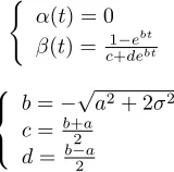
(t) = 0 (t) = _c1_+deebtbt

8 < :

b= pa2_{+ 2} 2

c=b+a

2

d=b a₂

The parameters a and can be obtained either from mortality tables, or, as we will do below, on sample, censored data. In both cases they can be calibrated by minimizing the mean squared error between the theoretical and actual probabilities: in the mortality table case the actual probabilities are the table ones, while in the sample case they are the empirical ones, as obtained, for instance, by the classical Kaplan-Meier procedure for censored data.

4

Copula estimate and best …t choice

In this section, we describe the procedure of estimating an Archimedean copula under censoring. In some respects, the approach in this paper is common to Denuit et al. (2004), who apply it to loss-ALAE data in non-life insurance.

1_{These probabilities are decreasing in agetif and only if}

ebt( 2+ 2d2)> 2 2dc

4.1

The distribution function of the Archimedean copula

Let Z = S Tm

x ; Tyf . De…ne K as the distribution function of Z. Note that

we have thatZ=C(U; V)where (U; V)is a random couple with unit uniform margins, andC the copula.

Genest and Rivest (1993) have shown that, for Archimedean copulas, with generator , this distribution functionK is given byK(z) =z (z), where

( ) = 0( )

( ); 0< 1: (9) The functionK is to be estimated from the data. We will make a distinction between complete data, such as in Denuit et al. (2001), and censored data, such as the application shown in this paper.

4.1.1 General principle without censoring

Genest and Rivest (1993) have shown that, for complete data of sizen, K can be estimated byKbn, de…ned as

b

Kn(z) =

1

n#fijzi zg wherezi=

1

n 1# x(j); y(j) x(j)< x(i); y(j)< y(i) ; where the symbol#indicates the cardinality of a set and x(i); y(i) ; i= 1; :::; n

are the observed data.

4.1.2 Wang-Wells empirical version of the generator in the presence of censored data

Wang and Wells (2000) have proposed a modi…ed estimator ofK for censored data. SinceKcan be written as

K(v) = Pr S T_xm; T_yf v =EhI_fS(Tm x ;T

f y) vg

i

;

the estimator is given by

b

Kn(v) =

Z 1

0

Z 1

0

I_fSb(s;t) vgdSb(s; t); (10)

where Sb stands for a nonparametric estimator of the joint survival function, taking censoring into account. For Sb we will use the estimator introduced in Dabrowska (1988).

4.1.3 Dabrowska’s estimator

Denote by Sbm _{and S}bf _{the Kaplan-Meier estimates of the univariate survival}

functions ofTm

of the event that observations x(i) and y(i), respectively, will be uncensored.

Furthermore, de…ne

b

H(s; t) = 1

n# i x(i)> s; y(i)> t ;

b

K1(s; t) =

1

n# i x(i)> s; y(i)> t; 1i = 1; 2i= 1 ;

b

K2(s; t) =

1

n# i x(i)> s; y(i)> t; 1i = 1 ;

b

K3(s; t) =

1

n# i x(i)> s; y(i)> t; 2i = 1 ;

and

b₁₁(s; t) =

Z s u=0

Z t v=0

b

K1(du; dv)

. b

H u ; v ;

b10(s; t) =

Z s u=0

b

K2(du; t)

. b

H u ; t ;

b01(s; t) =

Z t v=0

b

K3(s; dv)

. b

H s; v :

Dabrowska’s estimator is:

b

S(s; t) =Sbm(s)Sbf(t) Y

0<u s

0<v t

(1 L(₄u;₄v)); (11)

with

L(₄u;₄v) = b10(4u; v )b01(u ;4v) b11(4u;4v) 1 b10(4u; v ) 1 b01(u ;4v)

; (12)

with ₄u = u u , and₄v =v v . Then b11(4u;4v) is de…ned as the

estimated hazard function of double failures (i.e. deaths) at point(u; v), while

b10(4u; v )andb01(u ;4v)are the estimated hazard functions of failures of

(x)at uand (y)at v, respectively, given the exposed to risk de…ned at(u; v). The principle of equation (12) can be derived from the numerator. We match the expected number of joint failures in case of independence, with the actual number of joint failures. A negative di¤erence implies positive association. We de…ne

F(s; t) = Y

0<u s

0<v t

(1 L(₄u;₄v)); (13)

4.2

Estimating Kendall’s tau under censoring

Let Kendall’s tau be denoted by . Since for Archimedean copulas = 4

Z 1 0

( )d + 1; (14) we have that can be expressed in terms ofK in the following way:

= 3 4

Z 1 0

K( )d : (15) The estimated from (15) is suitable for censored data as well.

4.3

Estimation of generator

We can estimate by means ofK. Letbn be the empirical estimate of . Then,

for v ₂ (0;1); bn(v) = v Kbn(v). For each generator listed in Table 1, we

estimate the parameter through equations (9) and (14), with derived from (15). This leads to functions _b. We de…neK _b(v) =v _b(v), and choose the generator whose K _b has a minimum distance to Kbn. In this paper, the

distance is de…ned in a quadratic sense as a mean squared error, denoted by

M SE.

M SE _b =

Z 1 0

K _b(v) Kbn(v)

2

dv: (16)

4.4

Omnibus procedure

The procedure described above leads to the choice of the “most appropriate” Archimedean copula, with parameter corresponding to Kendall’s tau. To check the correctness of the procedure, for the same copulas the parameter is estimated through the pseudo-maximum likelihood or omnibus procedure. This method has been described in broad terms by Oakes (1994). Its statistical properties are analyzed in Genest et al. (1995).

The procedure treats marginal distributions as nuisance parameters of in…-nite dimension. The margins are estimated nonparametrically by rescaled ver-sions of the Kaplan-Meier estimators, with the rescaling factor (multiplier) equal to n/(n+ 1). The loglikelihood function to be maximized, denoted by L( ), has the following shape:

L( ) =

n

X

i=1

2

4 1i 2i ln [c (ui; vi)] + (1 1i) 2iln h

@C (ui;vi)

@v

i

+ 1i(1 2i) ln

h

@C (ui;vi)

@u

i

+ (1 1i) (1 2i) ln [C (ui; vi)]

3 5;

where(ui; vi) = Sbm(xi);Sbf(yi) ,C (ui; vi)is the copula under consideration,

andc (ui; vi) its density (i.e. the derivative with respect to both arguments).

5

Application to the Canadian data set

5.1

Description of the data set

We have used the same data set as Frees et al. (1996), Carriere (2000) and Youn and Shemyakin (1999, 2001). The original data set concerns 14,947 con-tracts in force with a large Canadian insurer. The period of observation runs from December 29, 1988, until December 31, 1993. Like the aforementioned papers, we have eliminated same-sex contracts (58 in total). Besides, like Youn and Shemyakin (1999, 2001), for couples with more than one policy, we have eliminated all but one of those (3,435 contracts). This has left us with a set of 11,454 married couples.

Since, as explained in Section 3, the methodology for the marginal survival functions applies to single generations, we have focused on a limited range of birth dates, both for males and females. In doing this, we have also taken into consideration the fact that the average age di¤erence between married man and women in the sample obtained after eliminating same sex and double contracts, is three years. In focusing on a generation and allowing for the three-year age di¤erence, we have considered only one illustrative example; however, the pro-cedure can evidently be repeated for any other couple of generations. We have selected the generation of males born between January 1st, 1907 and December 31, 1920 and those of females born between January 1st, 1910 and December 31, 1923. These two subsets, which amount to 5,025 and 5,312 individuals respec-tively, have been used for the estimate of the marginal survival functions. Then, in order to estimate joint survival probabilities, we have further concentrated on the couples whose members belong to the generation 07-20 for males and 10-23 for females. This subset includes a total of 3,931 couples. Both individuals and couples are observable for nineteen years, because they were born during a fourteen year period and the observation period is …ve years.

On this data set, we have adopted the general procedure sketched in Section 3 for the margins and the one in Section 4 for the joint survival function.

We have …rst obtained the empirical margins, using the Kaplan-Meier method-ology. These margins feed the Dabrowska estimate for the empirical joint sur-vival function. Starting from it, the best …t analytical copula has been estimated using the Wang and Wells (2000) method, as based on the approach by Gen-est and RivGen-est. Like Denuit et al. (2004), we have performed a check of the parameters and of the best …t choice using the omnibus procedure.

The marginal Kaplan-Meier data have been used also as inputs for the cali-bration of the analytical marginal survival functions, according to the method-ology in Luciano and Vigna (2005).

5.2

Kaplan-Meier estimates of marginal survival functions

The Kaplan-Meier maximum likelihood estimates of the marginal survival prob-abilities are collected in Table 2.

We notice that, di¤erently from both Carriere (2000) and Frees et al. (1996), we can calculate the empirical survival probabilities tpxonly untilt= 19. This

is due to the limited range of birth dates of our generations, coupled with the …ve year length of observation. Based on the explanation above, we take the initial agexto be 68 for males, 65 for females.

5.3

The bivariate survival function (Dabrowska)

Given the empirical margins in Table 2, provided by the Kaplan-Meier method, we reconstruct the joint empirical survival function using the Dabrowska esti-mator. We have simpli…ed the estimator by truncating to integer durations. This means that e.g. a duration of failure ofk (integer) corresponds to death betweenk andk+ 1. As data of death between durations5and6 were incom-plete (due to the maximal period of observation of 5.0075 years), we did not consider any deaths more than …ve years after the start of the observation.

In Table 3 we present the multipliers F(s; t), as de…ned in equation (13). Due to the time frame of observation of …ve years, we cannot explicitly compute the multipliers for durations greater than …ve. As usual with censoring, for durations greater than the observation period, we take the multiplier computed for the maximal duration.

We notice that all the multipliers are greater than one. This indicates posi-tive association and con…rms our intuition about the dependency of the lifetimes of couples. Later on, we will provide an exact measure (Kendall’s tau) of the amount of association.

Another relevant feature of the data, which can be captured from the table, is the fact that the multipliers are generally increasing per row and per column: this means that the amount of association is increasing. Namely, it means that, for given survival time of one individual in the couple, the conditional survival probability of the other member is more and more di¤erent from the unconditional one as time goes by. It also means that with a longer period of observation, we would probably have faced a stronger association between the two lives.

5.4

The copula choice (Wang & Wells)

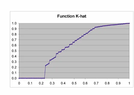
Figure 1

We observe that K^(v) is zero for v < 0:23; because the smallest value of

S(s; t)isS(19;19) = 0:23 (recalling that the presence of this minimum in turn is due to censoring and to the restriction to one generation, which reduces the observation window to 19 years).

The empirical K is used, according to formula (15), in order to calculate an estimate of the Kendall’s tau. We get = 0:71172, in line with the values obtained, for the same Canadian set, but without focusing on a generation, by other authors (Frees et al., 1996, Carriere, 2000, Youn and Shemyakin, 1999, 2001, Shemyakin and Youn, 2001).

The estimated provides us with the parameter values needed for imple-menting the theoretical copulas: as explained in Section 4.3, for each generator we obtain its parameter .

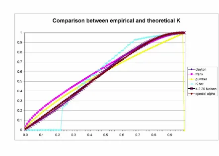
best copula. The graphical comparison can be done using Figure 2, where we present the theoreticalK’s and the empirical one.

Figure 2

We also compute the distance of each theoretical function from the empirical one, i.e. the mean square error M SE in (16), both starting from v = 0 and starting fromv= 0:23. By so doing, we obtain the errors in Table 4.

Both from the graph and the errors we conclude that the best …t copula is the 4.2.20 Nelsen’s one.

5.5

Omnibus procedure

As a further check of our selection, we implement the omnibus or pseudo-maximum likelihood procedure described in Section 4.4. As inputs for it, we use again the Kaplan-Meier marginal probabilities in Table 2. Table 5 presents the estimated parameters for each copula, their standard errors and the maximized likelihood function.

The maximum likelihood is maximized in correspondence to the Nelsen cop-ula: this procedure then con…rms the results of the Wang and Wells one. How-ever, contrary to the mean square error above, the di¤erence between maximized likelihoods is very weak: it ranges from 0.03% to 3%.

Also, the omnibus approach con…rms the validity of the Kendall’s tau esti-mates obtained with the Wang and Wells’approach: using the above standard errors, for each copula parameter and consequently for the Kendall’s tau -we computed a 95% con…dence interval around the maximum likelihood one. The Kendall’s tau of the Wang and Wells’method falls only in the con…dence interval of the Nelsen copula.

5.6

The analytical marginal survival functions

The couples of the data set have dates of birth between 1884 and 1993: even though in the papers which have dealt with the same data set the same law of mortality is assumed to apply for any life of the same gender, irrespective of the date of birth, we distinguish di¤erent generation survival probabilities and di¤erent intensity processes.

Contrary to Luciano and Vigna (2005), however, we take as a generation not a single age of birth, but thirteen consecutive of them, as speci…ed above: this assumption is based on the one side on the possibilities of reliable calibration (number of data) o¤ered by the present data set; on the other side, by the fact that there is not a unique de…nition of generation, and, generally speaking, persons with ages of birth close to each other are considered to belong to the same generation.

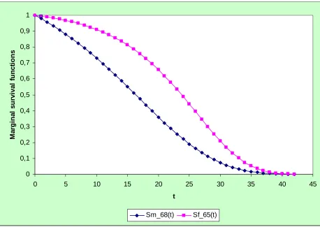
We have chosen the generation 1907-20 for males, initial age 68, and 1910-23 for females, initial age 65. We therefore present only two survival functions, which will be denoted asS₆₈m(t); S₆₅f (t)respectively. Their analytical expression is given by (8), where the estimated parameters are, respectively for males and females

a68= 0:0810021; 68= 0:00005; a65= 0:124979; 65= 0:00005

while the initial intensity values are

68(0) = 0:0204276; 65(0) = 0:0046943

Regarding the values of 68(0)and 65(0), according to Luciano and Vigna

survival probability of a Canadian insured male born in 1920 and aged 68 and with p65being the survival probability of a Canadian insured female born in

1923 and aged 65. However, this data is not available. Therefore, we have used the Canadian data set outlined above, and estimated with the KM method

p68 males and p65 females with all data available from the data set, without

restrictions on the generation. This has been done in order to have an estimate of those survival probabilities as accurate as possible (also considering the fact that the observation period is only …ve years, and therefore the individuals entering the method for the calculation of the survival probabilities were born in a six years interval).

The two survival functions are presented in Figure 3.

0 0,1 0,2 0,3 0,4 0,5 0,6 0,7 0,8 0,9 1

0 5 10 15 20 25 30 35 40 45

t

Ma

rgina

l

s

ur

v

iv

a

l

fun

c

tions

Sm_68(t) Sf_65(t)

6

The analytical joint survival function, its

as-sociation and long term dependency

We couple the …tted marginal survival functions of Section 5.6with the best …t copula choice of Section 5.4, according to the formula

S(x; y) =C(S₆₈m(x); S₆₅f (y)) with

C (u; v) = ln exp(u + exp(v ) e)

1

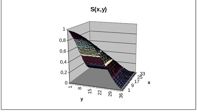
By doing so, we obtain the joint survival function S(x; y)of Figure 4, whose sections are presented in Figures 5 and 6 respectively

1 ₈

15 ₂₂

29 ₃₆

19

1725 33

0 0,2 0,4 0,6 0,8 1

y

x

S(x,y)

S(x,y), y fixed

0 0,1 0,2 0,3 0,4 0,5 0,6 0,7 0,8 0,9 1

0 10 20 30 40

x

y=1

y=5

y=10 y=15

y=20

y=25

y=30 y=35

S(x,0)=S(x)

S(x,y), x fixed

0 0,1 0,2 0,3 0,4 0,5 0,6 0,7 0,8 0,9 1

0 10 20 30 40

y

x=1

x=5

x=10

x=15

x=20

x=25

x=30

x=35

S(0,y)=S(y)

Figure 6

Looking at Figure 5, we notice that the smallery, the closer S(x; y)to the marginal distributionS(x;0) =S(x). On the other hand, ify is high,S(x; y)is almost ‡at until a certain agex_bafter which it decreases. This is due to the fact that the probability for the female of survivingy years, with highy, is very low and this a¤ects to a great extent the joint probability of survivingxyears for the male andy years for the female (even when the probability S(x;0) is very high becausex is small). After age _bxthe joint probability starts to decrease because of the joint e¤ect of low probability of survivingy years for the female andxyears for the male.

For Figure 6 the same comments made for Figure 5 apply. Notice that, while the agex_bafter whichS(x; y),y …xed, starts to decrease is always smaller than the …xed value of y (e.g. y = 35 =_{) b}x= 31; y = 30 =_{) b}x= 25; y = 25 =₎

b

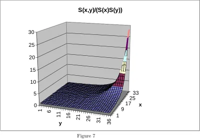
In Figure 7, we report the ratio between the joint survival function and the probability which we would obtain under the assumption of independence (the “classical” one): _SS_(x(x;y_)S()_y).

1 ₆

11 _{16 21}

26 ₃₁

36

1 9

17 25

33

0 5 10 15 20 25 30

y

x

S(x,y)/(S(x)S(y))

Figure 7

In doing this, please notice that we use the short notationSm₆₈(x) =S(x); S₆₅f (y) =

S(y). Figure 7 reports the time dependent measure of association 1(x; y) as

de…ned in (1), i.e. the joint survival probability as proportional to the inde-pendence case. The ratio is monotone in each argument and reaches very large values for largexandy. Note that for any(x; y), ₁(x; y)takes values between 1 and 1

max(S(x);S(y)). The lower bound is due to the positive association

mea-sured above, since1 corresponds to the independence case. The upper bound corresponds to the limit reached by the ratio when the joint survival function reaches the Fréchet upper bound, namelyS(x; y) = min (S(x); S(y)):

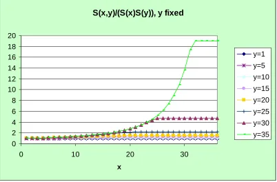
S(x,y)/(S(x)S(y)), y fixed

0 2 4 6 8 10 12 14 16 18 20

0 10 20 30

x

y=1

y=5

y=10

y=15

y=20

y=25

y=30

y=35

S(x,y)/(S(x)S(y)), x fixed

0 5 10 15 20 25 30

0 10 20 30

y

x=1

x=5

x=10

x=15

x=20

x=25

x=30

x=35

Figure 9

All the curves start at 1 for x = 0 or y = 0 and increase monotonically until a certain value, de…ned asx in Figure 8 and y in Figure 9, from which they remain constant. This suggests that the behaviour of the sections is quite similar to the curves corresponding to the Fréchet upper bound. Comparing the sections of Figure 8 with Figure 9 for the same …xed value, we observe that

x < y . This is probably due to the higher mortality experienced by males, compared to females.

Table 6 illustrates the measures _2x(0; y)and _2y(x;0)as de…ned in equa-tion (2). Column 2 displays the relative increase of the condiequa-tional expected remaining lifetime of (x), given that (y) survives to y, which, as explained in Section 2 increases as a function ofy. We have thatE[Tm

x ] = 16:51. Similarly,

column 4 shows the relative increase of the conditional expected remaining life-time of(y), given that(x)survives tox, now increasing as a function ofx. The unconditional life expectancy E Tf

y is equal to 21:92. We observe that, for

x=y, _2x(0; y)< _2y(x;0) for small values ofxor y but this inequality sign is reversed for large values of this argument.

As for the third measure of time-dependent association in Section 2, the cross-ratio function for the Nelsen copula, as a function ofS(u; u)is

which is increasing as a function ofu, as also shown in Spreeuw (2006). Figure 10 gives a plot ofCR(v)versus1 v.

Note that CR(1) = 2:43472 and that CR(v)takes very large values for v

close to 0. Hence, for the Nelsen copula, members of a couple become more dependent on each other as they age. This seems to be a reasonable assumption for married couples.

7

Conclusions

This paper represents a …rst attempt to model the mortality risk of couples of individuals, according to the stochastic intensity approach.

On the theoretical side, we extend to couples the Cox processes setup, i.e. the idea that mortality is driven by a jump process whose intensity is itself a stochastic process, proper of a particular generation within a gender. The dependency between the survival times of members of a couple is captured by a copula, which we assume to be of the Archimedean class, as in the previous literature on bivariate mortality.

On the calibration side, we …t the joint survival function by calibrating separately the (analytical) margins and the (analytical) copula. First, we select the best …t copula according to the methodology of Genest and Rivest (1993), as extended by Wang and Wells (2000) to censored data. We obtain the so-called Nelsen copula and we con…rm its appropriateness with the so-called pseudo maximum likelihood or omnibus procedure.

The best copula is far from representing independence: this con…rms both intuition and the results of all the existing studies on the same data set. In ad-dition, since the best …t copula turns is the Nelsen one, dependency is increasing with age.

Then, we provide a calibration of the marginal survival functions of male and female selecting time-homogeneous, non mean-reverting, a¢ ne processes for the intensity and give them in analytical form. Di¤erently from Luciano and Vigna (2005), we base the calibration on sample insurance data and not on mortality tables. Coupling the best …t copula with the calibrated margins we obtain a joint survival function which is fully analytical and therefore can be extended, for the chosen generation, to durations longer than the observation period.

The main contribution of the paper is in the calibration of a joint survival function which incorporates stochastic future mortality for both individuals in a couple. The approach seems to be manageable and ‡exible, and lends itself to extensive applications for pricing and reserving purposes.

References

[2] Artzner, P., and Delbaen, F., (1992). Credit risk and prepayment option, ASTIN Bulletin, 22, 81-96.

[3] Bi¢ s, E. (2005). A¢ ne processes for dynamic mortality and actuarial val-uations,Insurance: Mathematics and Economics, 37, 443–468.

[4] Cairns, A. J. G., Blake, D., and Dowd, K. (2005). Pricing death: Frame-work for the Valuation and Securitization of Mortality Risk, to appear in ASTIN Bulletin.

[5] Brèmaud, P. (1981). Point processes and queues - martingale dynamics, New York: Springer Verlag.

[6] Carriere, J.F. (2000). Bivariate survival models for coupled lives. Scandi-navian Actuarial Journal, 17-31.

[7] Cherubini, U., Luciano, E., and Vecchiato, W. (2004). Copula methods in Finance, Chichester: John Wiley.

[8] Clayton, D.G. (1978). A model for association in bivariate life tables and its application in epidemiological studies of familial tendency in chronic disease incidence.Biometrika 65, 141-151.

[9] Dabrowska, D.M. (1988). Kaplan-Meier estimate on the plane.The Annals of Statistics 16, 1475-1489.

[10] Dahl, M. (2004) Stochastic mortality in life insurance: market reserves and mortality-linked insurance contracts,Insurance: Mathematics and Eco-nomics, 35, 113–136.

[11] Denuit, M., Dhaene, J., Le Bailly de Tilleghem, C. and Teghem, S. (2001). Measuring the impact of dependence among insured lifelengths. Belgian Actuarial Bulletin, 1 (1), 18-39.

[12] Denuit, M, Purcaru, O. and Van Keilegom, I. (2004). Bivariate Archimedean copula modelling for loss-ALAE data in non-life insurance. Discussion Paper 0423, Institut de Statistique, Université Catholique de Louvain, Louvain-La-Neuve, Belgium.

[13] Du¢ e, D. Filipovic, D. and Schachermayer, W. (2003). A¢ ne processes and applications in …nance, Annals of Applied Probability, 13, 984–1053. [14] Du¢ e, D., Pan, J. and Singleton, K. (2000). Transform analysis and asset

pricing for a¢ ne jump-di¤usions, Econometrica, 68, 1343–1376.

[15] Du¢ e, D., and Singleton, K. (1999). Modelling term structures of default-able bonds, Review of Financial Studies, 12,687-720.

[17] Genest, C, Ghoudi, K. and Rivest, L.-P. (1995). A semiparametric estima-tion procedure of dependence parameters in multivariate families of distri-butions. Biometrika 82, 543-552.

[18] Genest, C. and MacKay, R.J. (1986). Copules archimédiennes et familles de lois bidimensionelles dont les marges sont données.Canadian Journal of Statistics 14, 145-159.

[19] Genest, C. and Rivest, L.-P. (1993). Statistical inference procedures for bivariate Archimedean copulas. Journal of the American Statistical Asso-ciation 88, 1034-1043.

[20] Hougaard, P. (2000).Analysis of Multivariate Survival Data.Springer. [21] Lando, D. (1998). On Cox processes and credit risky securities,Review of

Derivatives Research, 2, 99–120.

[22] Lando, D. (2004).Credit Risk Modeling, Princeton: Princeton Univ. Press. [23] Luciano, E. and Vigna, E. (2005). Non mean reverting a¢ ne processes for stochastic mortality, ICER working paper and Proceedings of the XVth International AFIR Colloquium, Zurich,Submitted.

[24] Manatunga, A.K. and Oakes, D. (1996). A measure of association for bi-variate frailty distributions. Journal of Multivariate Analysis 56, 60-74. [25] Milevsky, M.A. and Promislow, S. D. (2001). Mortality derivatives and the

option to annuitise, Insurance: Mathematics and Economics, 29, 299–318. [26] Nelsen, R.B. (1999).An Introduction to Copulas, Lecture Notes in Statistics

139, New York: Springer Verlag.

[27] Oakes, D. (1989). Bivariate survival models induced by frailties.Journal of the American Statistical Association, 84 (406), 487-493.

[28] Oakes, D. (1994). Multivariate survival distributions.Journal of Nonpara-metric Statistics 3, 343-354.

[29] Shemyakin, A. and Youn, H. (2001). Bayesian estimation of joint survival functions in life insurance, In: Monographs of O¢ cial Statistics. Bayesian Methods with applications to science, policy and o¢ cial statistics, European Communities, 489-496.

[30] Schrager, D. F. (2005). A¢ ne stochastic mortality,to appear in Insurance: Mathematics and Economics.

[32] Wang, W. and Wells, M.T. (2000). Model selection and semiparametric inference for bivariate failure-time data.Journal of the American Statistical Association 95, 62-72.

[33] Youn, H. and Shemyakin, A. (1999). Statistical aspects of joint life insur-ance pricing.1999 Proceedings of the Business and Statistics Section of the American Statistical Association, 34-38.

FACULTY OF ACTUARIAL SCIENCE AND INSURANCE

Actuarial Research Papers since 2001

Report

Number

Date Publication

Title

Author

135. February 2001. On the Forecasting of Mortality Reduction Factors.

ISBN 1 901615 56 1

Steven Haberman Arthur E. Renshaw

136. February 2001. Multiple State Models, Simulation and Insurer Insolvency. ISBN 1 901615 57 X

Steve Haberman Zoltan Butt Ben Rickayzen

137. September 2001 A Cash-Flow Approach to Pension Funding. ISBN 1 901615 58 8

M. Zaki Khorasanee

138. November 2001 Addendum to “Analytic and Bootstrap Estimates of Prediction Errors in Claims Reserving”. ISBN 1 901615 59 6

Peter D. England

139. November 2001 A Bayesian Generalised Linear Model for the Bornhuetter-Ferguson Method of Claims Reserving. ISBN 1 901615 62 6

Richard J. Verrall

140. January 2002 Lee-Carter Mortality Forecasting, a Parallel GLM Approach, England and Wales Mortality Projections.

ISBN 1 901615 63 4

Arthur E.Renshaw Steven Haberman.

141. January 2002 Valuation of Guaranteed Annuity Conversion Options.

ISBN 1 901615 64 2

Laura Ballotta Steven Haberman

142. April 2002 Application of Frailty-Based Mortality Models to Insurance Data. ISBN 1 901615 65 0

Zoltan Butt Steven Haberman

143. Available 2003 Optimal Premium Pricing in Motor Insurance: A Discrete Approximation.

Russell J. Gerrard Celia Glass

144. December 2002 The Neighbourhood Health Economy. A Systematic Approach to the Examination of Health and Social Risks at Neighbourhood Level. ISBN 1 901615 66 9

Les Mayhew

145. January 2003 The Fair Valuation Problem of Guaranteed Annuity Options : The Stochastic Mortality Environment Case.

ISBN 1 901615 67 7

Laura Ballotta Steven Haberman

146. February 2003 Modelling and Valuation of Guarantees in With-Profit and Unitised With-Profit Life Insurance Contracts.

ISBN 1 901615 68 5

Steven Haberman Laura Ballotta Nan Want

147. March 2003. Optimal Retention Levels, Given the Joint Survival of Cedent and Reinsurer. ISBN 1 901615 69 3

Z. G. Ignatov Z.G., V.Kaishev

R.S. Krachunov

148. March 2003. Efficient Asset Valuation Methods for Pension Plans.

ISBN1 901615707 M. Iqbal Owadally

149. March 2003 Pension Funding and the Actuarial Assumption Concerning Investment Returns. ISBN 1 901615 71 5

M. Iqbal Owadally

150. Available August 2004

Finite time Ruin Probabilities for Continuous Claims Severities

D. Dimitrova Z. Ignatov V. Kaishev

151. August 2004 Application of Stochastic Methods in the Valuation of Social Security Pension Schemes. ISBN 1 901615 72 3

Subramaniam Iyer

152. October 2003. Guarantees in with-profit and Unitized with profit Life Insurance Contracts; Fair Valuation Problem in Presence of the Default Option1. ISBN 1-901615-73-1

Laura Ballotta Steven Haberman Nan Wang

153. December 2003 Lee-Carter Mortality Forecasting Incorporating Bivariate Time Series. ISBN 1-901615-75-8

Arthur E. Renshaw Steven Haberman

154. March 2004. Operational Risk with Bayesian Networks Modelling.

ISBN 1-901615-76-6

Robert G. Cowell Yuen Y, Khuen Richard J. Verrall

155. March 2004. The Income Drawdown Option: Quadratic Loss.

ISBN 1 901615 7 4

Russell Gerrard Steven Haberman Bjorn Hojgarrd Elena Vigna

156. April 2004 An International Comparison of Long-Term Care

Arrangements. An Investigation into the Equity, Efficiency and sustainability of the Long-Term Care Systems in Germany, Japan, Sweden, the United Kingdom and the United States. ISBN 1 901615 78 2

Martin Karlsson Les Mayhew Robert Plumb Ben D. Rickayzen

157. June 2004 Alternative Framework for the Fair Valuation of

Participating Life Insurance Contracts. ISBN 1901615-79-0

Laura Ballotta

158. July 2004. An Asset Allocation Strategy for a Risk Reserve considering both Risk and Profit. ISBN 1 901615-80-4

Nan Wang

159. December 2004 Upper and Lower Bounds of Present Value Distributions of Life Insurance Contracts with Disability Related Benefits. ISBN 1 901615-83-9

Jaap Spreeuw

160. January 2005 Mortality Reduction Factors Incorporating Cohort Effects.

ISBN 1 90161584 7

Arthur E. Renshaw Steven Haberman

161. February 2005 The Management of De-Cumulation Risks in a Defined Contribution Environment. ISBN 1 901615 85 5.

Russell J. Gerrard Steven Haberman Elena Vigna

162. May 2005 The IASB Insurance Project for Life Insurance Contracts: Impart on Reserving Methods and Solvency

Requirements. ISBN 1-901615 86 3.

Laura Ballotta Giorgia Esposito Steven Haberman

163. September 2005 Asymptotic and Numerical Analysis of the Optimal Investment Strategy for an Insurer. ISBN 1-901615-88-X

Paul Emms Steven Haberman

164. October 2005. Modelling the Joint Distribution of Competing Risks Survival Times using Copula Functions. I SBN 1-901615-89-8

Vladimir Kaishev Dimitrina S, Dimitrova Steven Haberman

165. November 2005.

Excess of Loss Reinsurance Under Joint Survival Optimality. ISBN1-901615-90-1

Vladimir K. Kaishev Dimitrina S. Dimitrova

166. November 2005.

Lee-Carter Goes Risk-Neutral. An Application to the Italian Annuity Market.

ISBN 1-901615-91-X

167. November 2005 Lee-Carter Mortality Forecasting: Application to the Italian Population. ISBN 1-901615-93-6

Steven Haberman Maria Russolillo

168. February 2006 The Probationary Period as a Screening Device: Competitive Markets. ISBN 1-901615-95-2

Jaap Spreeuw Martin Karlsson

169. February 2006 Types of Dependence and Time-dependent Association between Two Lifetimes in Single Parameter Copula Models. ISBN 1-901615-96-0

Jaap Spreeuw

170. April 2006 Modelling Stochastic Bivariate Mortality

ISBN 1-901615-97-9

Elisa Luciano Jaap Spreeuw Elena Vigna.

171. February 2006 Optimal Strategies for Pricing General Insurance.

ISBN 1901615-98-7

Paul Emms Steve Haberman Irene Savoulli

172. February 2006 Dynamic Pricing of General Insurance in a Competitive Market. ISBN1-901615-99-5

Paul Emms

173. February 2006 Pricing General Insurance with Constraints.

ISBN 1-905752-00-8

Paul Emms

174. May 2006 Investigating the Market Potential for Customised Long Term Care Insurance Products. ISBN 1-905752-01-6

Martin Karlsson Les Mayhew Ben Rickayzen

Statistical Research Papers

Report

Number

Date

Publication Title

Author

1. December 1995. Some Results on the Derivatives of Matrix Functions. ISBN 1 874 770 83 2

P. Sebastiani

2. March 1996 Coherent Criteria for Optimal Experimental Design.

ISBN 1 874 770 86 7

A.P. Dawid P. Sebastiani

3. March 1996 Maximum Entropy Sampling and Optimal Bayesian Experimental Design. ISBN 1 874 770 87 5

P. Sebastiani H.P. Wynn

4. May 1996 A Note on D-optimal Designs for a Logistic Regression Model. ISBN 1 874 770 92 1

P. Sebastiani R. Settimi

5. August 1996 First-order Optimal Designs for Non Linear Models.

ISBN 1 874 770 95 6

P. Sebastiani R. Settimi

6. September 1996 A Business Process Approach to Maintenance: Measurement, Decision and Control. ISBN 1 874 770 96 4

Martin J. Newby

7. September 1996.

Moments and Generating Functions for the Absorption Distribution and its Negative Binomial Analogue. ISBN 1 874 770 97 2

Martin J. Newby

8. November 1996. Mixture Reduction via Predictive Scores. ISBN 1 874 770 98 0 Robert G. Cowell.

9. March 1997. Robust Parameter Learning in Bayesian Networks with Missing Data. ISBN 1 901615 00 6

P.Sebastiani M. Ramoni

10. March 1997. Guidelines for Corrective Replacement Based on Low Stochastic Structure Assumptions. ISBN 1 901615 01 4.

11. March 1997 Approximations for the Absorption Distribution and its Negative Binomial Analogue. ISBN 1 901615 02 2

Martin J. Newby

12. June 1997 The Use of Exogenous Knowledge to Learn Bayesian Networks from Incomplete Databases. ISBN 1 901615 10 3

M. Ramoni P. Sebastiani

13. June 1997 Learning Bayesian Networks from Incomplete Databases.

ISBN 1 901615 11 1

M. Ramoni P.Sebastiani

14. June 1997 Risk Based Optimal Designs. ISBN 1 901615 13 8 P.Sebastiani H.P. Wynn

15. June 1997. Sampling without Replacement in Junction Trees.

ISBN 1 901615 14 6

Robert G. Cowell

16. July 1997 Optimal Overhaul Intervals with Imperfect Inspection and Repair. ISBN 1 901615 15 4

Richard A. Dagg Martin J. Newby

17. October 1997 Bayesian Experimental Design and Shannon Information.

ISBN 1 901615 17 0

P. Sebastiani. H.P. Wynn

18. November 1997. A Characterisation of Phase Type Distributions.

ISBN 1 901615 18 9

Linda C. Wolstenholme

19. December 1997 A Comparison of Models for Probability of Detection (POD) Curves. ISBN 1 901615 21 9

Wolstenholme L.C

20. February 1999. Parameter Learning from Incomplete Data Using Maximum Entropy I: Principles. ISBN 1 901615 37 5

Robert G. Cowell

21. November 1999 Parameter Learning from Incomplete Data Using Maximum Entropy II: Application to Bayesian Networks. ISBN 1 901615 40 5

Robert G. Cowell

22. March 2001 FINEX : Forensic Identification by Network Expert Systems. ISBN 1 901615 60X

Robert G.Cowell

23. March 2001. Wren Learning Bayesian Networks from Data, using Conditional Independence Tests is Equivalant to a Scoring Metric ISBN 1 901615 61 8

Robert G Cowell

24. August 2004 Automatic, Computer Aided Geometric Design of Free-Knot, Regression Splines. ISBN 1-901615-81-2

Vladimir K Kaishev, Dimitrina S.Dimitrova, Steven Haberman Richard J. Verrall

25. December 2004 Identification and Separation of DNA Mixtures Using Peak Area Information. ISBN 1-901615-82-0

R.G.Cowell S.L.Lauritzen J Mortera,

26. November 2005. The Quest for a Donor : Probability Based Methods Offer Help. ISBN 1-90161592-8

P.F.Mostad T. Egeland., R.G. Cowell V. Bosnes Ø. Braaten

27. February 2006 Identification and Separation of DNA Mixtures Using Peak Area Information. (Updated Version of Research Report Number 25). ISBN 1-901615-94-4

R.G.Cowell S.L.Lauritzen J Mortera,

Faculty of Actuarial Science and Insurance

Actuarial Research Club

The support of the corporate members

CGNU Assurance

English Matthews Brockman

Government Actuary’s Department

is gratefully acknowledged.