Light scattering study of attractive interactions in a model microemulsion system

Theses Thesis/Dissertation Collections

6-29-1992

Light scattering study of attractive interactions in a

model microemulsion system

Dawn M. Campbell

Follow this and additional works at:http://scholarworks.rit.edu/theses

This Thesis is brought to you for free and open access by the Thesis/Dissertation Collections at RIT Scholar Works. It has been accepted for inclusion in Theses by an authorized administrator of RIT Scholar Works. For more information, please [email protected].

Recommended Citation

Dawn M. Campbell

Submitted to the Center for Materials Science and Engineering, Rochester Institute of Technology,

Rochester, New York 14623

IN PARTIAL FULFILLMENT OF THE REQUIREMENTS FOR THE DEGREE OF

MASTER OF SCIENCE

Signature of Author

D

__a_w_n_M

__

June 29, 1992

Certified by _

Dr. Michael Kotlarchyk Thesis Supervisor

Accepted by _

Dr. Andreas Langner Thesis Committee

Accepted by _

Dr. Surendra Gupta Thesis Committee

Accepted by ___

LIGHT SCA'rl'ERING STUDY OF ATTRACTIVE INTERACTIONS IN A MODEL MICROEMULSION SYSTEM

I, Dawn M. Campbell, hereby grant permission to the

Wallace Memorial Library of RIT to reproduce my thesis in

whole or in part. Any reproductions will not be for

Dawn M. Campbell

Center for Materials Science and _Engineering,

Rochester Institute of _{Technology, Rochester,} New York

14623

Abstract

Static and dynamic (photon correlation _{spectroscopy)}

light _scattering studies were conducted on

AOT/WATER/n-DECANE microemulsions near room temperature. The molar

ratio of water to AOT was varied from W = _{20 to 30. The}

volume fractions of the studied microemulsions ranged

from $ = _{0.03 to 0.45. Static light}

scattering data was

modeled _by a _theory based on attractive perturbations to

hard spheres. From the model, values for _A, the

attractive perturbation to the second virial _coefficient,

were determined. It was found that A is an _increasing

function of W. Photon correlation spectra were analyzed

in terms of an adhesive sphere model to produce

corresponding values of _A, which were compared to the

statically determined A-values. The two methods produced

A values that were not in agreement within experimental

error, however the methods independently had reasonable

PAGE

ABSTRACT 3

TABLE OF CONTENTS 4

LIST OF FIGURES 6

LIST OF TABLES 7

ACKNOWLEDGMENTS 8

Chapter 1. INTRODUCTION

1.1 Introduction to field 10

1. 2 The problem and method 18

Chapter 2. LIGHT SCATTERING TECHNIQUES

2.1 Essentials of _{instrument setup} 20

2.2 Static light _scattering 25

2.3 Photon Correlation _Spectroscopy 28

Chapter 3. THEORETICAL BACKGROUND

3.1 Interpretation of Static Light 34

Scattering

3.2 Interpretation of PCS 45

Measurements

Chapter 4. THE EXPERIMENT

4.1 Sample preparation and 51

compositions

4.2 Experimental results 57

4.3 Interpretation of results 61

Chapter 5. CONCLUSION AND SUGGESTIONS FOR FUTURE 73

WORK

APPENDIX A. Start _up procedure 76

APPENDIX E. _Intensity curve _fitting instructions 82

APPENDIX F. Derivation of A vs. a equation 83

Reversed Micelle 1.2 15

Swollen Micelle _1.3 16

Reversed Swollen Micelle 1.4 17

Experimental _Set-up 2.1 21

Osmotic Pressure 3.1 37

Hard Sphere Potential 3.2 40

Micellar Interaction Potential 3.3 41

Square Well Potential 3.4 41

Adhesive Sphere Model 3.5 42

Rayleigh Ratio vs. (J) , W = 24.7 3.6 44

Autocorrelation Function 3.7 47-48

Dc vs. (J) , W

= _27.5

3.8 49

AOT Structure 4.1 51

Aot/Water/n-Decane Microemulsion 4.2 53

Static Light _Scattering Experimental Results 4.3 58

PCS Experimental Results 4.4 60

Overlap Volume of Micelles 4.5 61

A vs. a 4.6 63

A vs. (1 - a1/3)-1

4.6.1 64

Rayleigh ratio vs. <$> for W = ₁₈

4.6.5 65

Rayleigh ratio vs. (J) for W = _{30 4.7 66}

X vs. a for C = .65 and 1.1 4.8 69

Static Light Scattering: W and Aperture 2.1 24

I would like to express _my thanks to Dr. Michael

Kotlarchyk. His _guidance, support and encouragement

provided the motivational framework for this work. He

always had time for discussions and his patience was

limitless.

Through _{grants, scholarship} and assistantships _supplied,

in _{part, by} the Materials Science and _Engineering

department at the Rochester Institute of _Technology, it

was possible for me to continue _my education. To Dr. P.

Cardegna I extend _my thanks for his role in _securing this

aid and also for his continued _help and input.

I would like to thank Dr. V- Gupta and Dr. A. Langner for

lending their time in the role of thesis committee

members.

I greatly appreciate the _generosity exhibited _by Dr. M

Illingsworth and his students in the Inorganic _chemistry

laboratory at R.I.T for their time and use of the _rotary

his assistance in the _laboratory, to Mike Chen and Shawn

Amershak for their _intriguing conversation and

encouragement and to Bill VanDerveer for his technical

assistance.

I am _deeply grateful for the support of _my parents and

brother, their encouragement is superseded _{only by} their

understanding.

In addition, I would like to thank _Kathy Plec and _Patty

Chapter 1. INTRODUCTION

1.1 Introduction to the field

There have been previous studies on colloidal

systems that predict the basic interaction potential due

to interparticle forces. Micellar and microemulsion

suspensions have been appropriate systems for these

studies.1/2'3/4/5/6 _{Current belief is that}

microemulsions

which contain reversed swollen micelles have a _strong

short range attractive force due to the interpenetration

of the surfactant tails _residing on the surface of the

interacting particles.4

The AOT/Water/n-Decane

microemulsion system is considered to be a model system

because it achieves thermodynamic _stability with _only

three components near room temperature. This

microemulsion system has been studied _using various

techniques _including small angle neutron _scattering

(SANS)3, small angle _x-ray scattering (SAXS)6 and light

scattering4, to name a few. The present _study employs

static light scattering and photon correlation

spectroscopy (PCS), also called dynamic light scattering

(DLS), to study the interaction between particles in the

Light _scattering is a _{particularly appealing way} to

study microemulsion systems because it is non-destructive

and requires small sample volumes _{(approximately} 3 ml).

The _following section _briefly discusses colloidal

systems. Then the _subgroup of _{microemulsions,} and

micellar _{microemulsions,} in _particular, are discussed.

COLLOIDAL SYSTEMS:

"A colloidal system consists of a _finely dispersed

phase (or discontinuous phase) distributed uniformly in a

finely divided state in a dispersion medium (or

continuous phase)-"7

There are colloidal systems all

around us, for instance, fog is a discontinuous water

droplet phase in a continuous air phase and milk is a

discontinuous fat droplet phase in a continuous aqueous

phase. The dispersed phase in these colloidal systems

usually has dimensions in the range of 1

-1000 _nm, and

is _finely divided throughout the continuous phase. In

some colloidal systems, however, the dispersed phase

particles are much larger than 1000 nm, hence the limits

One type of a colloidal system is an emulsion. An

emulsion consists of a fluid dispersed phase in a fluid

dispersion medium. In most _instances, emulsions either

consist of aqueous droplets in _oil, a water-in-oil _(W/0)

emulsion, or an oil-in-water _(0/W) emulsion. Milk is an

example of a 0/W emulsion with fat droplets in an aqueous

medium whereas mayonnaise is an example of an W/0

emulsion with aqueous droplets in an oil medium.7

One factor that determines whether or not an 0/W or

W/0 emulsion forms is the ratio of the amounts of the two

phases present (the ratio of the phase volumes). In most

cases the dispersed phase is the phase which is present

in the lower amount. When an emulsion _forms, there is an

increase in free _energy in the system as well as an

increase in interfacial area between the two phases

present. The amount of work required for the emulsion

formation is determined _by the interfacial tension. As

the interfacial tension _decreases, so does the amount of

work needed to form the emulsion, so emulsions form more

readily as the interfacial tension decreases. In

addition, the attainable droplet size decreases as the interfacial tension decreases. In _fact, if the

interfacial tension of a system approaches _zero,

in these _{spontaneously} formed systems is very small (< 10

nm _diameter) and so the droplets scatter little light

which makes the dispersions clear. These systems that

are _formed

spontaneously are called _{microemulsions, they}

consist of at _{least three} components _{(e.g., oil,} water

and _{surfactant) and} are _{thermodynamically} stable. Some

microemulsions need a fourth component _{(cosurfactant)} in

order to achieve stability. One of the major _driving

forces for the intense _study of microemulsions in recent

years is their possible use in _tertiary oil recovery-7 In

addition there is a general academic interest in _learning

about the particle interactions in complex fluid systems.

The microemulsion structure _may be that of random or

very ordered lamellar sheets, bicontinuous, or _micellar,

to name a few. The experimental system chosen in the

present _study was a micellar _{microemulsion,} hence the

following text will give a brief introduction to the

structure and types of micelles.

A micelle can be formed with water and a surface

active molecule (surfactant). The surfactant is an

amphiphile which means it is a molecule _consisting of two

parts, "one portion is a hydrophobic hydrocarbon chain

existence of these _opposing properties in the same

molecule, when dissolved in a _solvent, is the origin of

the thermodynamic _driving force for micellar formation."8

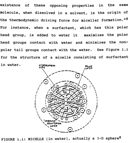
For _instance, when a _surfactant, which has this polar

head _group, is added to water it maximizes the polar

head groups contact with water and minimizes the

non-polar tail groups contact with the water. See Figure 1.1

for the structure of a micelle consisting of surfactant

in water. _td#o<UMc* COKE

^ "UNIOUNO*

".___"

N. COUNTXHION

XNLATCH

/

FIGURE 1.1: MICELLE (in water), actually a 3-D sphere8

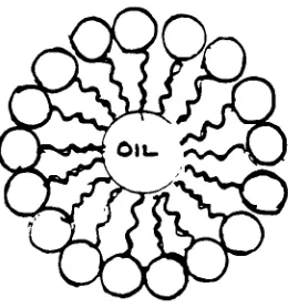
On the other hand, if the surfactant is added to a

hydrocarbon fluid (oil), the lower free _energy state is

obtained when the tail groups have maximum contact with

the hydrocarbon fluid and the polar head groups minimize

is called a reversed micelle. This structure is shown in the _{following figure.}

H --S.4A

FIGURE 1.2: REVERSED MICELLE (in hydrocarbon _fluid),

actually a 3-D sphere18

Not _only are there micelles and reversed _micelles,

there are swollen micelles and reversed swollen micelles.

A swollen micelle can be formed if another component is

added to the system. For example, _by adding a small

amount of oil to the micelle in water _system, a swollen

micelle is formed. Whether it is a swollen micelle or a

reversed swollen micelle is _generally dependent upon the

volume fractions of the components in the system. For instance, if a small amount of oil is added to the

micelle in water system, the oil situates itself such that it has maximum contact with the non-polar tail

maximum contact with the water. See Figure 1.3 for the

swollen micelle structure.

FIGURE 1.3: SWOLLEN _{MICELLE, actually} a 3-D sphere

Likewise, if a small amount of water is added to the

reversed micelle in hydrocarbon fluid _system, the water

pools _up in the center of the surfactant molecules due to

steric and electrostatic repulsive forces of the polar

heads as well as the hydrophobic effect. This is called

FIGURE 1.4: REVERSED SWOLLEN _{MICELLE, actually} a 3-D

1.2: Problem and Method

The adhesive hard sphere model has been shown to

accurately describe the short range attractive

interaction observed in some colloidal suspensions.5

Microemulsions _comprising of _AOT, water and oil have been

shown to exhibit a short range interaction potential due

to the _overlapping of the surfactant tails.2/3 The

effect of _changing the micelle dimension on the strength

of this interaction has not been previously examined in

detail.

The present _study employs a model that assumes an

attractive interaction between particles to analyze the

static light _scattering data. Photon correlation

spectroscopy data is analyzed _using the adhesive sphere

model. This adhesive sphere model has _previously been

applied to the AOT/Water/Oil microemulsion system in SAXS

studies.19/20/21 _{A major finding} in these _studies is

that the interaction potential changes with the droplet

concentration. In _fact, the stickiness was found to

decrease significantly with increasing water volume

fraction.20 _{In the} present _study, the _relationship

water to AOT molar _{ratio, which is related to the}

size of

Chapter 2. LIGHT SCATTERING TECHNIQUES

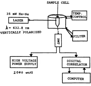
2.1 Essentials of Instrument Setup:

A model SP127-35 35 mW Helium-Neon laser with

wavelength = _632.8

nm was used with a Brookhaven

Instruments BI-200SM Goniometer version 2.0. The

goniometer houses a high _quality glass vat in which there

is decahydronapthalene _(decalin), an index _matching

fluid. The decalin was supplied _by Aldrich Chemical Co.

Inc. with > 99% purity- In the center of the vat is a

holder for a 12mm nominal diameter round sample cell. An

EMI-9863 photomultiplier tube _(PMT) with a reported dark

count of 20 counts/sec was used to detect the scattered

light. The PMT is powered _by a 0

-3000 volt EG&G ORTEC

high voltage power _supply set at 2050 volts. The signal

is then sent to a BI-2030AT Digital _Correlator, with 136

real time data channels and 6 real time _delay channels,

and a BI computer for processing. The index _matching

fluid and the samples are kept at constant temperature

using a Fisher Scientific _Isotemp Refrigerated circulator

Model 9000 with

0.1

C accuracy. In _addition, a BI

filtration system was used for _filtering the index

matching fluid in the vat. See Figure 2.1 for an

35 mW _He-Ne

LASER

>

SAMPLE CELL

^= _{632.8 nm}

VERTICALLY POLARIZED

HIGH VOLTAGE POWER SUPPLY

2050 volXS

TEMP.

PZSCONTROL

N

DIGITAL CORRELATOR

1

T"

COMPUTER

FIGURE 2.1: EXPERIMENTAL SETUP USED FOR STATIC LIGHT

SCATTERING AND PHOTON CORRELATION SPECTROSCOPY STUDIES.

The alignment of the system should be checked

alignment was checked at least once a _month, when no

significant variances were observed at the _scattering

angle of 90 , the alignment was checked _{approximately}

once _{every three} months. _Also, in the summer months when

the weather proves to be _{increasingly detrimental,} the

alignment was checked more _frequently, on the order of

once or twice a week. The procedure for _checking the

alignment is outlined in the Light _scattering manual

provided _by Brookhaven Instruments _{Corporation10,} in the

alignment _section, page 7-4 through 7-8. It should be

noted that at 90 no significant effects were observed

when the sample cell was positioned so that a scratch was

in the region where the beam enters the cell as opposed

to a region where there were no scratches (no bright

spots _observed) on the sample cell. It is believed that

scratches on the sample cell will have an effect on

experimental results if the experiment employs small

scattering angles.

The index matching fluid (decalin) has an index of

refraction that is approximately equal to that of the

glass vat and the glass sample cell. The purpose of this

fluid is to _keep the _incoming laser beam from _scattering

when it encounters the vat-liquid and liquid-sample cell

experimental period was the original fluid put in the

system. The decalin was filtered approximately once a

month for the first four months then once _every four

months thereafter. _Filtering the decalin reduces the

amount of _{impurities in the} system however it introduces

bubbles. This presents a problem as decalin is a rather

viscous fluid and it was found that it took at least one

week for the bubbles to either settle on the floor of the

vat or rise to the surface where _they would not be in the

path of the beam _(heating the fluid in the vat _using the

temperature controller accelerates the elimination of

bubbles to a certain degree). Thus the index _matching

fluid was _only filtered when it was _absolutely necessary.

It is the opinion of this student that the decalin

should be replaced no less than once a year. This

procedure should be done with all appropriate protective

equipment and in the _company of another in case of an

accident.

The temperature was kept constant at 23.1 C and

the PMT was positioned at 90

for both PCS and static

light scattering experiments. An aperture setting of

200 yfm was used for all photon correlation _spectroscopy

autosample time selection (press ALT START). For the

static light _{scattering experiments the} sample time was

fixed at l jusec and the aperture was adjusted as shown in

table 2.1.

TABLE 2.1: STATIC LIGHT SCATTERING

w APERTURE _(Jim)

20.0 400

24.7 400

27.5 400

29.0 200

29.5 200

NOTE: The duration was adjusted for each sample so that

IO5

counts accumulated over the total duration

period. On the average, the duration was 200

2.2 STATIC LIGHT SCATTERING:

Static light _scattering has been used extensively in

the _study of micellar and microemulsion systems.2/4

Static light _scattering provides a non-destructive _way to

extract information about interparticle interactions. In

the present _study, static light _scattering experiments

were performed on AOT/Water/n-Decane microemulsions in an

effort to learn about the attractive interactions

exhibited _by the reversed swollen micelles.

Essentials of Static Light Scattering:

A laser is focused such that it illuminates the

sample under study. Each particle in the sample scatters

light. The photomultiplier tube (PMT), is positioned at

a particular angle (90 for the present study) in order

to detect the number of photons emitted at the detector

angle. This photon count is updated for a prescribed

time period.

Ultimately, it is the total photon count or actual

number of photons _being scattered from the particles for

measure. The _scattering angle and temperature were kept

constant for this study.

However, the measured photon count rate is dependent

upon the _geometry of the _system, (how far the detector is

from the _sample, for example). In order to compare

results from different systems it is desirable to obtain

a value from the measured photon count rate of the sample

that _only depends on the scatterer _itself, and not on the

source or the detector optics. _{By calculating} the so

called Rayleigh _{factor, geometry} considerations are

eliminated. The Rayleigh factor is defined as follows:10

i?C9) =^2 rl (2.1)

/. V iw vob

!(-&-) = _{scattered radiance}

r = _{distance from} the detector

vobs = illuminated volume !inc = incident irradiance

The Rayleigh factor has units of cm~1steradian~1

.

This represents "the fraction of light scattered per unit

length per unit solid angle."10

Typically this Rayleigh

factor is called a Rayleigh ratio, but since it does have

units, it is not strictly correct to call it a ratio.

this paper will continue _using it to avoid _unnecessary

confusion.

The Rayleigh ratio is not _{directly measured,} the

photon _count/sec, (or count _rate), is _measured, therefore

corrections must be made to the measured count rate.

Also the photometer is not an absolute photometer so it

must be adjusted for inherent dark counts. See

reference #10 for details. The light _scattering

equipment had _vertically polarized light. The index

matching fluid-to-vat refractive indices ratio was

sufficiently close to 1 and the ratio of the refractive

indices of the solvent and calibration liquid _(toluene)

was also close to 1. The system was _non-aqueous, and the

solution to cell interface produced no significant

reflection. With all the above conditions the Rayleigh

ratio is calculated _using the _following formula:

m

Rai

-f ?" '

frf"

** _1calL*3J

~JDCR

where: R(-. ₎ = _Rayleigh ratio of sample at -O-. Rcal(90

) = _absolute Rayleigh ratio of

calibration liquid at 90

Toluene = _14.0 * 10~6 cm"1

Isample( "^"

) = _count rate of the sample at the detector angle -O*

.

2.3 PHOTON CORRELATION SPECTROSCOPY:

Photon correlation _{spectroscopy (PCS),} or dynamic

light _{scattering (DLS), has become a useful tool in}

determining the diffusion coefficient and the particle

size distribution of materials _having particles with

dimension of a few nanometers to several micrometers.

Some advantages of _using PCS over other methods that

determine the diffusion coefficient are that the

measurement does not require calibration and it is _easy

to operate the equipment and perform the experiment. In

fact, as _long as the suspension is _sufficiently dilute

(negligible interparticle interactions or multiple

scattering) , determination of the diffusion coefficient

is independent of particle composition and

concentration.11 _{In this particular}

study, the samples

were not of such low concentrations that the particles

did not _interact, so this interaction contributes to the

particle motion. There are also hydrodynamic

considerations; the movement of the molecules in the

fluid creates a perturbation in the fluid _which, in _turn,

Essentials of PCS:

A laser is focused such that it illuminates a

relatively dilute suspension. Each particle in the

solution scatters light. These light waves interfere

with each other and produce a net _{scattering intensity,}

I(t), which is detected _by the photomultiplier tube

(PMT). Each particle's position in the suspension

fluctuates _randomly due to Brownian motion _(diffusion) ,

interparticle interactions and hydrodynamic

contributions. This random fluctuation in position

produces a random fluctuation in the phases of each

scattered wave as _they arrive at the PMT. This means

that as the particles diffuse in the _suspension, the

intensity, I(t), fluctuates in a _way that is related to

the particle motion.

An efficient _way to analyze this _fluctuating

intensity signal is to use correlation. Most people are

familiar with the idea of correlation. "If two variables

or two signals are _highly correlated, then a change in

one can be used to predict, with _confidence, the change

in the other. Mathematically, correlation is defined

quantities."10 _if

you _{multiply the}

intensity function _by

a _delayed

version of _itself and average the _quantity,

it is called an _{autocorrelation}

function, C(t).

CCO = _-t^/GO

+ICr+Oy

Here _{I(*r )} is the count rate at time T , and I(f +t) is

the _intensity at some later _time, n plus _delay time t.

For small time intervals the correlation between I(T ₎

and _{I(T+t) is high but as the}

delay time _{(t) increases,}

the correlation decreases. In _fact, the correlation

function decays _{exponentially} for a suspension of _rigid,

globular particles and is given by:10 *

CCO = e(-2ZW0

, (2.4)

where _q is the _scattering wave vector defined as follows:

- _*

4-ffJ

(2.5)

* _{For a more} rigorous explanation of the autocorrelation

In Eq. _2.5, n is the index of refraction of the solvent, is the wavelength of light in vacuum and is the

scattering angle. _{Therefore, by}

analyzing the _intensity autocorrelation _function, the collective diffusion coefficient can be determined.

The autocorrelation function described in Eq. 2.4 is based on the system _having monodisperse particles.

However, most systems are _{significantly} polydisperse and

this means that each particle size contributes its own exponential term. Therefore the autocorrelation function

for a polydisperse system contains an integral of the

exponential in Eq. 2.4. This, of _course, increases the

complexity of _solving the autocorrelation for the diffusion coefficient.10/12/13 _{For a system of}

polydisperse particles, the autocorrelation function now

looks like:10

00

t

CCO = GCl) e"rt

dT . (2.5.5)

0

Here G is a distribution function, and V = _Dq2. This Laplace transform equation has a nontrivial solution. Experimental data is hindered by the effect of

dust, real measurement noise and real baseline drifts.

the exponential makes this a _difficult problem to solve.

The system used for this _study uses the method of

cumulants to analyze the integral and extract the desired

distribution information.

The method of cumulants makes no assumption about

the form of the distribution function. A Taylor series

is used to expand the exponential about the mean value.

The series is integrated _yielding a general result.

"This result shows that the logarithm of the

autocorrelation function can be expressed as a polynomial

in the sample _time, t. The coefficients of the powers of

t are called the cumulants of the distribution. In

practice, only the first couple of cumulants are obtained

reliably, and these are identical to the moments of the

distribution. (In general, the first moment of _any

distribution is the average and the second is the

variance.)" 10

From the first and second moments of the

distribution, the diffusion coefficient is calculated. It

may be calculated _using either a calculated or measured

baseline subtraction. The calculated baseline is the

infinite time value of the correlation _function, whereas

channels. If the difference between the two baselines is

less that _0.02%, the measured baseline may be used,

otherwise use the calculated baseline. In this _study the

Chapter 3. _{THEORETICAL BACKGROUND}

3.1 Interpretation of static light _scattering

measurements

The properties of a dilute colloidal system are

similar to those of an ideal gas. _Hence, an _analogy can

be made between the two systems. The Ideal Gas Law

states :

P

kg

where: P =

pressure

kB = _Boltzmann

constant

T = _{absolute temperature} P = _#

density of gas molecules.

For non-ideal gases, however, there are particle

interactions which add terms to Eq. 3.1 as shown below:

j- =

p ?

[B2cn

*

t

+...] .

<3-2> B

If however, a _very dilute system of gases is _considered,

Eq. 3.2 can be truncated after the first _interaction

term:

= _p

[i

p] .

(3.3)

To make the _{analogy between} a _very dilute gaseous

system and a dilute colloidal _{system, specifically} a

micellar colloidal _system, the pressure _(P) is analogous

to the osmotic _pressure,

TT

^

molecules per unit volume of _container) is analogous to

the number of micelles per volume of solution. This

equals the volume fraction of the dispersed phase ₍ <J) ₎

per volume of one micelle _{(Vm)), i.e.,}

kBT Vml 2

"J

where B is called the second virial coefficient.

If the micelles are assumed to be a constant size

then it is known that the intensity of _vertically

polarized light scattered _by particles in a continuous

phase is4

/C9) = KVm<t>Stq) PC?)

. (3.5)

JC9}= _intensity at the _scattering angle

Vm = _volume of micelle

<p = micellar volume fraction

S(q)= structure factor

K is defined as

*-.*.'[]'(V)

(3-6)

The particles used in the present _study have radius

under 10 _nm, so the intraparticle form _{factor, P(q)} , is

essentially equal to l.4

Also, in the limit as _q

approaches _zero, the structure factor _S(q) is related to

the osmotic pressure _by the _{compressibility} relation4

k T

SCO) = --|-^ I (3.7)

TO

m*

Where:

[~

<9IlT = compressibility of system (isothermal

!:

]

J osmotic compressibility) .

In order to evaluate Eq. _3.7, the osmotic pressure

must be known. To understand osmotic pressure it is

useful to see Figure 3.1 which exhibits a container that

is divided _by a semipermeable _membrane, (permeable _only

to solvent) . On one side of the membrane there is pure

solvent, and on the other side is a microemulsion.

Closing the microemulsion side is a piston which can

is the applied pressure required to _stop the solvent from

going through the membrane.

Soi_vc/JT

/fti_{d^oe/ijit-S/ih PiStoa.}

FIGURE 3.1: The osmotic pressure ₍ II) is the pressure

required to _stop solvent from _going through the membrane.

Now _returning to Eq. 3.4, which relates the osmotic

pressure to the second virial coefficient and the volume

fraction, it is known that this second virial coefficient

is related to the interaction potential as follows:4

00

B=--f\

[eC-*M/V0

-l]

r* dr

(3.8)

One of the main conclusions of the modern fluid

theories used to explain microemulsion experimental

results is that steric repulsions between close particles

is a large _determining factor in the spatial structure.

Using a perturbation to the hard sphere potential is one

technique used to deal with attractive or repulsive

interactions. In _fact, Calje et al.9

proposed that the

hard sphere potential _(UHS) added to the attractive

potential _(UA) , describes the interaction potential

between micelles. Carnahan and Starling14 proposed an

equation of state that describes the hard sphere

contribution to the osmotic pressure. The total osmotic

pressure is defined as2

n= nHS+

^

The Carnahan-Starling expression states that for a hard

sphere gas the equation of state is14

^S

*2V)/Cl-^3]

Now, using the analogy presented above for a

non-ideal gas compared to a hard sphere fluid, Eq. 3.10 can

nHS

*HS

VHS

, (3.11)

where (&= _volume

fraction of hard spheres

Vj,s= _volume

of a hard sphere.

The attractive osmotic pressure must also be considered.

If it is treated as a _{perturbation, it is} 4

kDT n. = VB

4

f

kQT _Vm

J

UA

UA(r) is the attractive portion of the interaction

potential. The hard sphere volume _fraction, ,^HS _, is

related to the total volume _{fraction, $}

, by

(3.14)

Using the total osmotic _pressure, the second virial

coefficient is calculated to be B = _{8a +}

A, where A is as

defined in Eq. 3.13 and is the attractive _{perturbation to}

the second virial coefficient. In this model the photon

count rate is4

/ce) =

KVm

{l+4a<>

V

V

? *4<>Cl +a*)

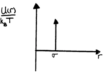
Pictorially the hard sphere interaction is as shown

in Figure 3.2.

(Jko

*a

FIGURE 3.2: HARD SPHERE _POTENTIAL, there is infinite

repulsion when the spheres are in contact

(the distance between the center of the

spheres is <r ) and zero interaction potential when o~ < r < oo .

In the hard sphere model the interaction potential is

infinitely repulsive when the spheres are _touching and as

soon as their contact breaks _{(moving apart) ,} there is

zero interaction potential. _However, there are micelles

in the microemulsion, not hard _spheres, and

experimentally the interaction has been shown to be of

kJ~

FIGURE 3.3: Micellar interaction potential

One _may consider _modelling this micellar system with

a square well attractive interaction potential as shown

in the _following figure.

UcO

kBT . i

1"

H WlOTH Or

WfcH-FIGURE 3.4: Square well potential

The square well potential requires a range parameter to

describe the width of the well in addition to _knowing the

diameter of the particles the depth of the well and a

constant. This presents a rather complex problem

involving four _fitting parameters. The adhesive sphere

The adhesive sphere model has been shown to

effectively describe the microemulsion interaction

potential throughout a large range of volume fractions in

SAXS experiments.19/20/21 _{This model is shown in Figure}

3.5.

T

FIGURE 3.5: Adhesive sphere model for the interaction potential. The attractive well is

infinitely narrow (let d approach <T ).

The range parameter is eliminated _{by letting} the

width of the attractive potential, (d - 0"

), approach

zero. This makes the attractive range _infinitely narrow.

Baxter15 _{has defined the interaction potential for the}

ILLrJ = kBT JLirfx.

r < _(f

J^Ll2tM-o-)/^(]

< r < d

O _{r > d}

This model has been _successfully used in previous

experiments.1/21

Robertus, et. al.19

have used the

adhesive sphere model and considered the effects of

polydispersity. The potential shown above has a

singularity when d = fl"

, however the second virial

coefficient, (Eq. 3.8), remains finite due to the

exponential term.16 The parameter

*C

stickiness parameter. It is _positive, dimensionless and

is is equal to 2/A. Since A is a measure of the

stickiness of the particles, the inverse of t. is also

a measure of the stickiness between particles.

By fitting an experimental photon count rate

vs. <f> curve with Eq. 15, the attractive perturbation to

the second virial coefficient (A), and _(a), the ratio of

the hard sphere volume fraction to the total volume

fraction, can be determined. Remember that the measured

photon count rate is not independent of the _geometry of

the experimental setup, therefore the measured photon

plotted against the volume fraction. See Figure 3.6 for

an example of a typical Rayleigh ratio vs. (J) curve.

(B).

a.ooe-s

2

U

^>s.ooe-5

-*^

o

I

x4.00C-S

-o

?

i

.2.0OE-5

i

W - _24.7

A = _6.004

a

O.OOC+0 ]iii nm iiiiiiiiiiiiii iimiiii

0.00 0.05 0.10 0.1S

0

nii|iiimiimini

0.20 0.25 olo

FIGURE 3.6: Rayleigh ratio vs. volume fraction for an H20/AOT/Decane microemulsion with

3.2 Interpretation _{of PCS}

measurements

At _{relatively low concentrations the collective}

diffusion coefficient is described as follows:16/17

Dc = DQ[ _{1 +}

kf) , (3.17)

where _Dc is the collective diffusion coefficient, _D0 is

the Brownian or single particle diffusion coefficient

and _lp is the volume fraction of particles in the

suspension. k is a numerical coefficient that depends on

particle interactions. _Using the adhesive sphere _model,

k is dependent on the stickiness parameter ₍ L describes

the adhesion between _interacting surfactant _tails) as

shown below:1

k = 1.454

-[yp)

The single particle diffusion coefficient _D0 is

described _by the Stokes-Einstein relation which states

that as the particle diameter _decreases, the _diffusivity

increases:

Dn =

kBT

0 =

i7r7r-.

Here, +} is the shear _viscosity of the solvent, and _rn is

the _{hydrodynamic radius of the}

particles, which are

assumed to be spherical in shape.11

When the diffusion

coefficient is _known, equations 3.17 and _3.19, are used

to calculate the effective diameter.

Throughout the _relatively low range of volume

fractions _prepared, the diffusion coefficient was

calculated for each sample batch of particular micelle

size. The diffusion coefficient is calculated _using the

method of cumulants from the _intensity autocorrelation

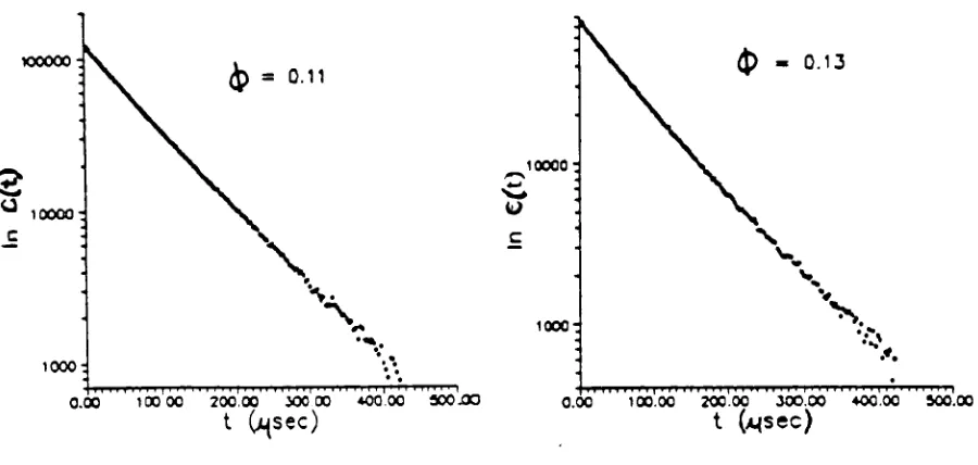
data. Typical autocorrelation functions are shown on the

following pages (Figure _3.8) These are plotted on a semi

10000

u

c

1000

10000

-u

c

1000

III II111II1 1 I IIIIII 1 11 1II

0.00 100.00 200.00 30000 40000 500.00 t _(t\sec)

100:

0.00

I III I IIIIII 100.00 20000 200.00 4O0.0C

t _(i^sec)

o

c

4>

10000:

/

1000:

\fa

o.cA 100.00 W0.00 300.00 400.

-1000000:

$

t _(i{sec)

cr 100000:

(i(sec)

WOOOO

= 0.11

3

o 10000

1000

(J> - _0.13

10000:

U

c

looo:

I|I_|IIII IIIlI|IIIIII III|llI IIIIII_|'I II I M I' 0.00 100 00 200.00 300CO 400.00 500jOO

t _(^sec)

I|| | |I I I I_|IMII I I I I|II III I I I II'II I I I I'I1I'II I I I I I₍

0.00 100.00 200.00 300.00 400.00 500.00

t _(>qsec)

FIGURE 3.7: The natural logarithm of the

intensity autocorrelation function.

This data is used to calculate

the collective diffusion coefficient,

At a given _W, the diffusion coefficient was plotted

against the volume fraction. A best straight line fit

was drawn _using

only the low volume fraction data (this

is because higher order terms were dropped in the

theoretical _development) . The _resulting curve was

extrapolated to zero concentration to find D0. A typical

example is shown in the _following figure.

(B).

XCC-7

W - _27.5 A - _7.11

+-.08

O.CC+0

o o o 0 o 0

FIGURE 3.8: Batch _10, W = _{27.5, Using photon}

correlation spectroscopy the diffusion

coefficient was obtained for each volume

fraction. _Only one trial was performed.

From Eq. 3.17, the slope of the curve is equal to

kD0. Knowing the slope and _D0, the value for k can be

determined. _Knowing k and Eq. _3.18, the stickiness

parameter, C , can be determined. From the stickiness

virial _coefficient) can be calculated. The value for A

determined _using PCS can be compared to the value

Chapter 4. THE EXPERIMENT

4. 1 Sample preparation _and

compositions

A swollen reversed micelle system was chosen for

this study. The three component microemulsion consisted

of _H20, AOT which is Bis(2-ethylhexyl)sulfosuccinate

sodium _salt, and n-decane (a ten carbon chain oil). The

surfactant _(AOT) has a branched tail configuration.

Figure 4.1 shows two AOT molecules with their tails

overlapping. Sample compositions were specified _by

choosing the water to AOT molar _{ratio, (W)} , as well as

the AOT-plus-water volume fraction of the solution ₍ <J) ₎ .

The chemical formula for AOT is C2oH37Na07S. The water

to AOT molar ratio was _determined as follows:

V._waterPvtter

W -I"

water]

= MMwatef

I AOT] Aot

MMAOT

vwater = _volume

of water

r}water = density of water = _{1 g/cc}

^water =

molecular mass of water = _{18 g/mole}

mAOT = _mass

of AOT

^AOT =

molecular mass of AOT = _{444.5 g/mole.}

The size of the reversed swollen micelles _linearly

increases with W. The surface area is determined _by the

amount of AOT present and the size of the reversed

swollen micelle is _directly related to the surface area.

In _addition, as W changes the _density of micellar

droplets changes. The other factor _determining the

composition of the microemulsion is

tp

fraction of micelles (water + _AOT) :

Vwater

mAOT

[j^\

Vwater

\J~^\ +

VDtcane

An oversimplified _{illustration of the} particular

microemulsion used is shown in the _following figure.

FIGURE 4.2: AOT/water/decane microemulsion: Contains

swollen reversed micelles

Sample preparation is _decidedly the most difficult

portion of the experiment. _Accuracy is _critical, however

even with _accurately made _samples, the results can be

obscured _by impurities. It is critical that impurities

be minimized, as _they scatter light and make it

difficult, if not impossible, to distinguish _scattering

from the particles in solution.

It was found that _{significantly} different results

purified AOT. The unpurified results were erratic and

drifted over time. Thus for all reported results,

samples were made with purified AOT. See APPENDIX D for

the AOT purification _procedure.

We used 18 M -TL deionized water supplied _by the

R.I.T. A-level science stockroom. The AOT was supplied

by Fluka with > 99% purity. The decane was supplied _by

Aldrich with >99% purity. In _addition, the samples were

each filtered _using Gelman Sciences ACRODISC LC PVDF 0.2

jum pore size syringe filters. _They were filtered twice

through the same filter.

All samples were made _{by diluting} a stock solution

to the desired volume fractions. The diluted samples were

put in glass containers. Each sample was poured into a

sample cell cleaned _according to _cleaning procedure #1

(see APPENDIX C). The _cap was placed on the sample _cell,

the cell was _lightly shaken and the microemulsion poured

into a disposable 10 ml syringe fitted with a 0.2 j^m

filter. The solution was filtered into the sample _cell,

shaken and poured back into the syringe to be filtered

for the second time. The sample was _visually inspected

for impurities, and if present the solution was filtered

to equilibrate _thermally to 23.1

C and stabilize. This

takes about 24 hours.

The sample batches were prepared _according to W,

which is related to particle size. For a particular

batch the W value was kept constant and the volume

fraction ranged anywhere from

$

4.1 shows the composition of the original stock solution

for each sample batch. Doped decane was added to

calculated amounts of the stock solution to achieve the

desired volume fraction. The decane was doped to 0.02

weight percent in order to _stay above the critical

micelle concentration (the concentration of surfactant

TABLE 4.1: SAMPLE COMPOSITIONS

BATCH # H20

cc

AOT

g

DECANE

CC

W

Of

STOCK

B5 10.000 9.9950 56.500 24.7 0.25

B6 14.600 12.0003 46.800 30.0 0.35

B7 8.910 11.0046 34.620 20.0 0.35

B8 7.300 10.0120 30.000 18.0 0.35

B8.1 6.850 9.4024 18.540 18.0 0.45

B9 9.110 15.0002 41.570 15.0 0.35

BIO 16.870 15.1446 56.220 27.5 0.35

Bll 17.617 15.0012 57.370 29.0 0.35

4.2 Experimental results

From static light _scattering, experimental results

for the Rayleigh ratio vs. volume fraction were obtained.

See Figure 4.3 for the static light scattering

experimental results. Notice that A is an _increasing

function of W. The error bars shown in graphs A and B

represent the _{reproducibility} between two _trials, which

is _{approximately} 15%. The circles in these two graphs

represent the average of the trials and the error bars

show the maximum and minimum values. Graphs C-E were

constructed on the basis of a single trial.

This data was put into a _fitting program (See

APPENDIX _E) which fits the data to Eq. 3.16 _using a chi

square minimization routine to get the best fit. From

the best fit curve, values for _A, (the attractive

perturbation to the second virial _{coefficient),} and _a,

(the ratio of the hard sphere volume fraction to the

(A).

ue-s, W - 20 A - _4.795

, a - _0.454 3_1.0C-9 .B.0C-CI

i

K 8.0E-9

-0

m i

52 <4.0E-3

-1

2.0E-S

-0.DO 0.

1 1 1 1 1 1 1 1 1 II M 1

io o.io oJo 0.40 0 (E). 2.0E-4 U ^1J-4 O

I

i

W - _29.5

A = _9.081

a - 0.724

O.OE+O

-jiniliihi1 1 ni J "I"' ""''1,

0.00 0.05 0.10 0.13 oiO 0.23 OJO 0

(B).

s.oe-5-, W = _24.7

A - _6.004

a = _0.701 o ^.OE-5 o

I

i

I II I 1 1 1 1 111 1 1 1 1 1 1 1 111 1 1 1 I M I 1 1 1 1 1 1 II11 111 1 1 1 111 1II1 1 " ' ""I 0.00 0.09 0.10 0.13 0.

0 (D). y2-0E-4: g X g y 1.0E-4-c$ C9S.0E-S 5 O.OE+O

W - ₂₉

A = _10.134

a = _0.783

j thi mimtm nn iniMTTMTtn hiiiiiiiiiihhiiiiiii.iiiim

0.00 0.05 0.10 0.15 0-20 0.25 OJO

0

FIGURE 4.3:

Graphs A-E show the dependence of the Rayleigh ratio on thevolume fraction.

They are displayed in order of _increasing W. Experimental data are represented

with circles. Graphs A and B have error

bars which show _{the reproducibility}

between two trials. Graphs C-E were

constructed on the basis of a single trial. The theoretical fit to the data,

From PCS experiments, data for the relationship

between the diffusion coefficient and volume fraction of

AOT/WATER/n-DECANE microemulsions were obtained. This

data is _graphically presented in Figure 4.4. The fit was

done _manually to low volume fractions. From the slope

and _intercept, k and _D0 are determined respectively.

Knowing k, the stickiness parameter is calculated (see

Equations _3.17, 3.18 and 3.19). From the stickiness

(A). _(B).

iOE-7n

W - _24.7

A - _{7.1 S +-J0}

(C).

3.0E-7

W - 29.0

A - 7.44 +- .08

0.OE+O"

1 1 ii 1 1 iiiii1 11 11 1 i111i i1 1 1 > 1 1ii > 1 1 1 1 1 i 11

0.00 0.10 oio OJO 0.40

l-7

W - _27.5

A - _7.11 +- .08

O 0 0

0 0 0

O.OE+O-M ITT HTI

T|IT 1 II.I I I I I 11I I ITT III TI I II I f I1

0.00 0.10 0.20 OJO 0.40

0

W - 30.0

A - 7.01 +- .08

0

FIGURE 4.4: From PCS, the relationship between the diffusion coefficient and was

determined. Experimental data is

shown with circles and the theoretical

4.3: Interpretation of results

Huang et.al.3

suggest that as two micelles approach

one another the surfactant tails are able to penetrate to

a certain _extent, this is the cause of the adhesiveness

or attractive portion of the interaction potential. See

Figure 4.5.

OVERLAP voi-umiT

WKjh)

o^-miu

FIGURE 4.5: The assumption is that there is a maximum penetration depth (h) due to the

branching structure of the AOT tails. It

is also assumed that A, the attractive

perturbation to the second virial coefficient, is proportional to the

overlap volume V(R,h). The total radius

is equal to R and the surfactant tails

It can be determined that the attractive

perturbation to the second virial coefficient equals

A= C ZL

H

h

2 _(4.3)

where C is a constant. See Appendix F for a derivation

of this equation.

The values for A and a obtained from the theoretical

fit to the static light _scattering data (Rayleigh

ratio vs. <f> ) were plotted to see if

they obeyed the

relationship described in Eq. 4.3. To do this a data

point was picked at low _a, the a-value and it's

corresponding A-value were put into Eq. 4.3 where the

(-h/2) term was omitted as it has a negligible affect on

the outcome of the A value. _Also, the _(3L) and the

proportionality were incorporated into the constant C

which makes the _fitting equation of the form

A =

1

-a2

(4.4)

With the data point _{(a, A)} put in the _equation, it

was solved for C. For this low "a"

was also _picked, and _solving for _C, a value of 1.1 was

calculated.

Using these two C _{values, curves were generated}

according

to Eq. 4.4. These curves are displayed _along with the

data in Figure 4.6.

100.00 n

80.00

60.00

-40.00

-20.00 :

0.00 1 1 1 1 i 1 1 1 1 ₁ 1 1 1 1 1 1 1 1 11 1 1 1 1 1 1 1 1 1 ₁1 i 1 1 1 i i i1 ₁ 1 1 1 1 1 1 1 1 i₎

0.00 0.20 0.40 0.60 0.80 1.00

FIGURE 4.6: The attractive perturbation to the second virial coefficient as a function of the

ratio of the hard sphere volume fraction

to the total volume fraction.

Experimental data are displayed with

circles and the generated "theoretical"

The actual C value is believed to lie within the range of

0.65 < _C < 1.1 . It was realized later that a better

way to find the constant C would be to plot A vs.

(1 - a1/3)"1

. Using Eq. 4.4, a straight line fit to the

points yields a slope that equals C. This is shown in

Figure 4.6.1.

12.00 -a

10.00 -.

8.00

'-< 6.00

'-4.00 -.

2.00 -.

(2=0.1?

000 : i i i i i i ii i| i i i iir i i i| i i i ir i i i i | ii i i i i i i i l 066 4.00 8.00 .,12.0016.00

( 1

-a*)

FIGURE 4.6.1: A best straight line was drawn to yield

C = 0.78. This falls well within the

previously-Due to time _limitations, the actual critical points for a

and <P were not found from Figure 4.6.1. However, the

constant C is _definitely within the range of C-values

obtained earlier.

The range of W values from which data was obtainable

was limited. With W < 18 , the intensity was so low it

was difficult to get a photon count and the curve did not

have a _bending over trend observed with the other light

scattering data. See Figure 4.6.5.

1.0E-5

P8.0E-6

<

a: 6.0E-6

X

LiJ 4.0E-6

CH O 2.CE-6

<

W = ₁₈

O.OE+O

o o

, i ,i |mimiiii|"i 111 1 n 111 1 1111i 1₁ 0.00 O.io 0.20 0.30 0.40 0.50

<t>

On the other _hand, when _running a sample batch with W =

30, the static light _scattering data was _highly erratic

and it was not possible to fit the data _using Eq. 3.15.

This data is shown in the _following figure.

J.OC-4, W = ₃₀

o

\2.5-4

-22-0C-4A

< 0.

-j-1.3-4:

g

jf1.0E-4 :

s.oe-3-.

0.0C-H3 : '

I J II III IIII11

000 0.10 o.io o.io oio

*

FIGURE 4.7: Static light _scattering data unable to be fit using Eq. 3.15.

It is believed that there is a phase change _occuring

somewhere between W = _{29.5 and W} = _{30 that is}

causing the

eratic trends observed in the W = _{30 data.}

Thus, W's

were chosen to fall in the range of 20 to 29.5. As

displayed in Figure _4.3, the static light _scattering data

for W = _29.5 follows the trend of the theory. This leads

one to believe that there may be a critical point

The critical points are defined _by the conditions:

La

J

= o

(4.5)

and

d2

n

d

f

= 0

(4.6)

Using Eq. 3.9, 3.11, and 3.12 it can be shown that first

derivative of the osmotic pressure with respect to the

volume fraction is

an _ 1+ Aa<j>

+

Aa2<j>2 - 4

qfy3

+ a

V

4

(4.7)

3 ₊ Cl-ac*)4 *

The second derivative of the osmotic pressure with

respect to the volume fraction is

32n_ Aa

*Sa2<fi

-UaH2

+Aa

V

-a& *- AA<j>aCl

-a<j>^ 3

d<t>2 Cl-o^)4

[l+

V

V

+^Cl

-a^D

4]

Using the constraint in Eq. _4.4, the first and

second derivatives were set equal to zero. The constant

C was set equal to 0.65 and 1.1. A range of a-values were also chosen. The vertical coordinate in these graphs _(x)

represents a_<p . These curves are shown in Figure 4.8.

The curves indicated that the critical a-value lies

within the range 0.82 < a <0.90 .

From the critical X and _a-values,

(J)c

&<-.

0.144 <

d>c

17.39 <

he

Huang2, through an analysis that excluded the factor of

"a", found _Ac = _{21.2 and} (J)t = _{0.13. We believe the}

values above to be better representations of the actual values because the theory used accounts for the ratio of the hard sphere volume to the total volume of a

0.33

0.3

0.23

0.2

x _0.15

0.1

0.05 4. *

r-r.

!*.?

4 4) 4 i_ T 1 1 I

0.9 0.82 0.84 0.86 0.88 0.9 0.92 0.94 0.96 0.98 1

<K

C = _1.1

0.9 0.82 0.84 0.86 0.88 0.9 0.92 0.94 0.96 0.98 1

a,

Figure 4.8

X =

a$

Squares and pluses denote setting the first derivative .ofIT with respect to

< equal to zero

Diamonds represent _{setting the} second derivative ofIT with respect to

fy

critical point is where the first derivative curve crosses the second derivative curve. This is only an approximation due to the constant _C,which was obtained from _fitting the experimental

The critical values for A are plotted on the

following A vs. W graphs for both static light scattering

and PCS. The critical values seem to follow in the trend of the static light _scattering data. The PCS data

however, do not have _any noticeable relationship to the

5CO -I

< 10.00

-OOCOOSL3 EXPERIMENTAL VALUES

00000A _'CPITiCAL) FOR (t = ₆₅

aaaaaa _(critical; for c = _{1 1}

0 o o :o J 1 1 0 CO

0.00 CO 2O00

w

30 00

(>-)

20 CO

-i

- _{COCOCPCS EXPERIMENTAL} VALUES

1500 _{] 00000} A (CRITICAL) FOR =

.65

j aaaaaa _(CRITICAL) FOR C= _1.1

< 10.CO

-5.C0 -I

0.00 iii

C CO 10 00

o oo

I _| I I III i M II Tl 1

2000 30.00 *000

w

FIGURE 4.9: Static light _scattering and photon

correlation _spectroscopy calculated

values for the attractive perturbation

to the second virial coefficient as a

The values for A that were obtained from static

light _scattering ranged from A = _{4.795 to 10.134} and

seemed to correspond with the critical point analysis.

The values from PCS data ranged from A = _{7.01 to 7.44} and

did not exhibit _any particular trend. Although the A

values from the independent studies did not have exact

correspondence, they were _certainly in the same range.

The photon correlation _spectroscopy experiments were all

performed on a single trial basis. More trials would be

beneficial in the sense that _any erratic values would

have a diminished effect. In this experiment, PCS data

Chapter 5. CONCLUSIONS AND SUGGESTIONS FOR FUTURE WORK

From static and dynamic _(PCS) light scattering

results, it has been determined that the attractive

perturbation to a hard sphere model is capable of

describing the AOT/WATER/n-_{DECANE microemulsion. The}

agreement of the static light _scattering data with the

theory is quite good within the range of volume fractions

and W values that were _{experimentally} accessible. The

independently determined values for A _{using PCS,} although

not as _outstanding as the static light scattering,

confirmed that the values obtained are in reasonable

agreement.

I must question results that _Huang reports in

reference #2. He claimed to fit static light _scattering

data with a function that was dependent on _only three

parameters _(A, 4> , constant) . I tried to fit _my

experimental data with his function and was unsuccessful.

However, the four parameter fit which includes the

parameter, a, closely fit the data.

One of the limitations of the data analysis

presented in previous sections of this paper is that the

not seem to affect the conclusions. Experimental errors,

which were within _15%, are comparable to the effects of

the _{polydispersity} on the photon count at the volume

fractions examined.

Another _possibility is that there are _many

assumptions, including some about the hydrodynamic

aspects of the particle _diffusion, in the formulation of

Eq. 3.18 that predicts the value for k, the numerical

coefficient _affecting the collective diffusion

coefficient. The hydrodynamic aspects in particular are

difficult to calculate theoretically. _Or, it _may be as

simple as the _way the best line was fit to the PCS data.

The fit was done _manually to low volume fractions. There

is a lot of room for error in _deciding what constitutes

low volume fractions. Additionally, the fact that _only

one trial was performed made it difficult to draw a best

fit line because error bars were not present.

The results presented above are consistent with SANS

results3 _{which suggest} that the _overlapping of the

surfactant tails is the source of the short range

interaction potential observed. The strength of this

interaction is believed to be related to the _overlap

suggest that there _may be other contributors to the

strength of the interaction.

An exceptional area for future research would be to

s