C
2011. The American Astronomical Society. All rights reserved. Printed in the U.S.A.
OBSERVATIONS OF BINARY STARS WITH THE DIFFERENTIAL SPECKLE SURVEY INSTRUMENT. III.
MEASURES BELOW THE DIFFRACTION LIMIT OF THE WIYN TELESCOPE
∗Elliott P. Horch1,5,6, William F. van Altena2,5, Steve B. Howell3, William H. Sherry3, and David R. Ciardi4,5
1Department of Physics, Southern Connecticut State University, 501 Crescent Street, New Haven, CT 06515, USA;[email protected] 2Department of Astronomy, Yale University, P.O. Box 208101, New Haven, CT 06520, USA;[email protected] 3National Optical Astronomy Observatories, 950 North Cherry Avenue, Tucson, AZ 87719, USA;[email protected],[email protected]
4NASA Exoplanet Science Institute, California Institute of Technology, 770 South Wilson Avenue, Mail Code 100-22,
Pasadena, CA 91125, USA;[email protected]
Received 2011 February 3; accepted 2011 March 22; published 2011 April 28
ABSTRACT
In this paper, we study the ability of CCD- and electron-multiplying-CCD-based speckle imaging to obtain reliable astrometry and photometry of binary stars below the diffraction limit of the WIYN 3.5 m Telescope. We present a total of 120 measures of binary stars, 75 of which are below the diffraction limit. The measures are divided into two groups that have different measurement accuracy and precision. The first group is composed of standard speckle observations, that is, a sequence of speckle images taken in a single filter, while the second group consists of paired observations where the two observations are taken on the same observing run and in different filters. The more recent paired observations were taken simultaneously with the Differential Speckle Survey Instrument, which is a two-channel speckle imaging system. In comparing our results to the ephemeris positions of binaries with known orbits, we find that paired observations provide the opportunity to identify cases of systematic error in separation below the diffraction limit and after removing these from consideration, we obtain a linear measurement uncertainty of 3–4 mas. However, if observations are unpaired or if two observations taken in the same filter are paired, it becomes harder to identify cases of systematic error, presumably because the largest source of this error is residual atmospheric dispersion, which is color dependent. When observations are unpaired, we find that it is unwise to report separations below approximately 20 mas, as these are most susceptible to this effect. Using the final results obtained, we are able to update two older orbits in the literature and present preliminary orbits for three systems that were discovered byHipparcos.
Key words: binaries: visual – techniques: high angular resolution – techniques: interferometric – techniques: photometric
1. INTRODUCTION
In recent years, the use of CCDs and electron-multiplying CCDs in speckle imaging has led to a large number of magnitude differences of binary stars appearing in the literature (see, e.g., Horch et al.2004,2010,2011; Balega et al.2007; Tokovinin et al.2010; Docobo et al.2010). The linearity of these devices has permitted reliable photometric information to be obtained, at least under observing conditions where the decorrelation of primary and secondary speckle patterns due to the finite size of the isoplanatic patch can be assumed to be small. These magnitude differences should eventually pave the way for many robust comparisons with stellar structure and evolution models for the sample of “classic” speckle binaries, i.e., those with separations in the range ∼0.04–1 arcsec, a significant contribution which would not be possible without photometric information of the components in multiple filters.
However, the existence of reliable photometry in speckle imaging has another, perhaps more important, advantage: the ability to determine the shape of the speckle transfer function in detail, or equivalently, the average shape of the individual
∗ The WIYN Observatory is a joint facility of the University of Wisconsin-Madison, Indiana University, Yale University, and the National Optical Astronomy Observatories.
5 Visiting Astronomer, Kitt Peak National Observatory, National Optical
Astronomy Observatory, which is operated by the Association of Universities for Research in Astronomy, Inc. (AURA) under cooperative agreement with the National Science Foundation.
6 Adjunct Astronomer, Lowell Observatory, 1400 West Mars Hill Road,
Flagstaff, AZ 86001, USA.
speckles themselves. For example, if speckles are seen as blended or elongated due to a component below the diffraction limit, it should in theory be possible to retrieve the relevant astrometric and photometric information, if the data are taken with a linear detector. With older microchannel-plate-based systems, systematic errors in detection affect the detailed shape of the speckles obtained, adding a severe complication to the interpretation of the speckle profile. However, with seeing-limited images of high quality taken with linear detectors, it is possible to fit a blended stellar profile to a binary star model with reasonable accuracy. Of course, performing a binary star fit to such a profile is put on much more stable ground if the object is known or suspected to be binary by other means. The same should hold true with sub-diffraction-limited speckle observations of binaries: with linear detectors and high-quality observations, there is no need to view the diffraction limit as an absolute barrier when analyzing speckle data.
distinguish between residual atmospheric dispersion, which is color dependent, and the presence of a sub-diffraction-limited component, which is not.
In 2008, we built the Differential Speckle Survey Instrument (DSSI), a speckle imaging system that contains a dichroic ele-ment so that it takes data in two different filters simultaneously. The instrument itself is described in Horch et al. (2009, hereafter Paper I) and has the following advantages over single-channel speckle imagers: (1) twice as much data are taken per unit of time, which can be used either to increase the signal-to-noise ra-tio for astrometric measurement or to decrease the time needed to achieve a given signal-to-noise ratio, (2) a color measure-ment of the components of a binary system can be made in a single observation, and (3) taking data in two colors simul-taneously gives leverage on residual atmospheric dispersion, which is especially important for sub-diffraction-limited mea-surement. The first two items mentioned were discussed more fully in Horch et al. (2011, hereafter Paper II). In the current pa-per, we study the measurement accuracy and precision obtained with DSSI to date from sub-diffraction-limited observations. We also cull other relevant observations from work with our earlier CCD-based speckle imager, the Rochester Institute of Technol-ogy—Yale Tip-tilt Speckle Imager (RYTSI), and present those here as well. We will show that two-color speckle imaging is effective in producing accurate and reasonably precise astromet-ric data to separations below one-quarter of the diffraction limit under certain conditions, whereas our single-channel speckle observations are susceptible to systematic error at separations below 20 mas.
Thus, we argue that two-color speckle imaging can be an ex-tremely efficient and powerful technique for measuring small-separation systems, even from mid-sized telescopes such as WIYN. For example, at a distance of 100 pc, a separation of 10 mas (approximately one-quarter of the diffraction limit at WIYN) corresponds to a physical separation of 1 AU. With the advent of complete spectroscopic samples such as the Geneva–Copenhagen survey (Nordstr¨om et al. 2004), as well as spectroscopic work on cluster binaries, this presents an in-teresting opportunity to measure (if not resolve) the separations of such systems, and therefore to combine the spectroscopic, photometric, and astrometric data for many stringent tests of stellar structure and evolution in the years to come.
2. OBSERVATIONS AND DATA REDUCTION
The first speckle observations at WIYN with a CCD detector were taken in from 1997 to 2000 (Horch et al.1999,2002). This speckle system consisted of an optics package designed and built primarily by Jeffrey Morgan when he was working in the detector group headed by J. Gethyn Timothy at Stanford Uni-versity. Originally, this camera was mated with a multi-anode microchannel array detector, but a fast-readout Photometrics CCD camera was provided by Zoran Ninkov of Rochester Insti-tute of Technology in 1997 to explore the viability of CCD-based speckle observations at WIYN. However, the targets observed during this time frame were almost exclusively above the diffrac-tion limit of the telescope, and so no measures presented here come from this setup.
In 2001, we began using a system exclusively designed for CCD-based speckle imaging, RYTSI, designed and built pri-marily by Reed Meyer, two of us (E.H. and W.vA.), and Zoran Ninkov (Meyer et al.2006). As we gained greater experience with this system, we began to push the limits of the device, including observing some binaries when they were known to be
below the diffraction limit. The DSSI camera replaced RYTSI in 2008, and was used with two Princeton Instruments PIXIS 2048B CCD cameras until the beginning of 2010, whereupon these detectors were replaced with two Andor iXon 897 EM-CCD cameras. (Some data in 2009 were taken with the first iXon camera obtained on one port of DSSI with the other port vacant.) For a full description of the DSSI design and optical components, please see Paper I.
2.1. Basic Properties
To form the list of observations under consideration for the current work, we reviewed the archive of WIYN speckle data from the RYTSI period to the present and identified possible sub-diffraction-limited observations. We then used the same method of reduction and analysis as in our previous papers (most recently described in Paper II), i.e., the observations selected conform to the same data quality cuts as normal observations above the diffraction limit. This is a Fourier-based method, where a fringe pattern is fitted to the object’s spatial frequency power spectrum deconvolved by that of a point source. The region over which the fit is made is approximately an annulus in the Fourier plane. The inner region (representing the lowest spatial frequencies) was not fit due to the fact that it is dominated by the seeing disk, and small differences in seeing (at high signal-to-noise ratio) can greatly affect the final reduced-χ2of
the fit. On the other hand, the highest spatial frequencies (near and beyond the diffraction limit) are dominated by noise and can likewise affect the final fit in an adverse way. The outer boundary of the fit annulus is therefore set as a contour of constant signal-to-noise ratio.
In previous work, we applied a data quality cut such that the effective outer radius of the fit annulus times the separation was required to be above a certain value. This ensured that the observation was at or above the diffraction limit in high-quality observations, and for lower quality observations, it ensured that the observation displayed at least three fringes (a central and both first-order fringes) within the fit annulus, which we determined was needed to make certain that lower signal-to-noise observations had high-quality astrometry. Obviously, in the current work this particular data cut was relaxed, as even high-quality observations would exhibit only a central fringe before the diffraction limit was reached in the Fourier plane. Because of this, it is not unreasonable to expect that some loss of astrometric precision may occur in sub-diffraction-limited observations.
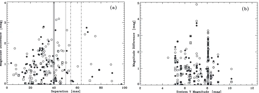
Figure 1.(a) Magnitude difference as a function of separation for the full set of measures described in the text, including those judged not to be of high enough quality to report. A handful of separation measures above 100 mas were present in the sample, but the plot has been truncated to clearly show the behavior at sub-diffraction-limited separations. (b) Magnitude difference as a function of systemVmagnitude for the same sample. In both plots, the open circles are measures taken with the 550 or 562 nm filter, filled circles are measures in the 698 or 692 nm filter, and squares are measures taken in the 754 or 880 nm filters. In (a), the two solid vertical lines mark the diffraction limit for 550 and 562 nm, the dotted lines mark the same for 692 and 698 nm, and the dot-dashed lines mark 754 and 880 nm.
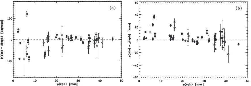
Figure 2.Measurement differences between paired observations plotted as a function of average measured separation,ρ. (a) Position angle (θ) differences and (b) separation (ρ) differences. In both plots, filled circles indicate results for paired measures with different filters and the same observation date, open circles are drawn when the two observations did not occur on the same date but during the same run, and squares indicate observations taken on the same date in the same filter. As in Figure1(a), the vertical lines mark the diffraction limit for the filters used; from left to right these are 550 and 562 nm (solid lines), 698 and 698 nm (dotted lines), and 754 and 880 nm (dot-dashed line).
identified, though again the sensitivity to magnitude difference falls off at fainter magnitudes. This can be understood in terms of signal-to-noise ratio and compared directly with Figure 1(b) of Paper II. The current figure has a very similar appearance though it appears shifted to the left (or in other words, toward brighter magnitudes) by approximately two magnitudes relative to work above the diffraction limit. We conclude that speckle observations below the diffraction limit are less sensitive both in terms of limiting magnitude and magnitude difference than those above the diffraction limit.
In Figure 2, we explore the astrometric repeatability of the sample by pairing observations wherever possible, either by using the simultaneous observations in the case of DSSI or sequential observations in pre-DSSI observations. (In the latter case, the second observation was only required to be during the same observing run as the first observation, not directly sequential in time.) Figure 2(a) shows the behavior of the position angle differences between each pair, while Figure2(b) shows the separation differences. Both are plotted as a function of the average separation obtained. The mean value for the position angle difference is Δθ = −6.◦7±2◦.8, while the subset of observation pairs taken in different filters, this is reduced to Δθ = −2◦.3 ± 1◦.9. For the subset of
observation pairs taken in different filters and simultaneously, the result is Δθ = −1◦.6 ±1◦.6. In separation, the average differences for the same three samples areΔρ=0.1±1.3 mas, Δρ= −0.7±0.6 mas, andΔρ= −0.6±0.6 mas, respectively. Turning now to the standard deviations for these three samples, we obtain σΔθ = 22◦.5±2.◦0,σΔθ = 13◦.1±1◦.3, and σΔθ = 9◦.3 ± 1.◦1 in position angle and σΔρ = 10.4 ±0.9 mas, σΔρ =4.3±0.4 mas, andσΔρ=3.5±0.4 mas. In general, these values appear to indicate that better repeatability is achieved when the observations are obtained simultaneously. There is also basic consistency between the position angle and separation values, as the average separation of the sample is approximately 30 mas and, at that separation, a linear measurement difference of 3.5 mas represents an angle difference of approximately arctan(3.5/30) ∼ 7◦, compared with the measured value of ∼9◦. The fact that the measured value is slightly larger than the linear prediction is easily explained by the smallest separation systems, where the predicted angle would be much larger than that of the average separation.
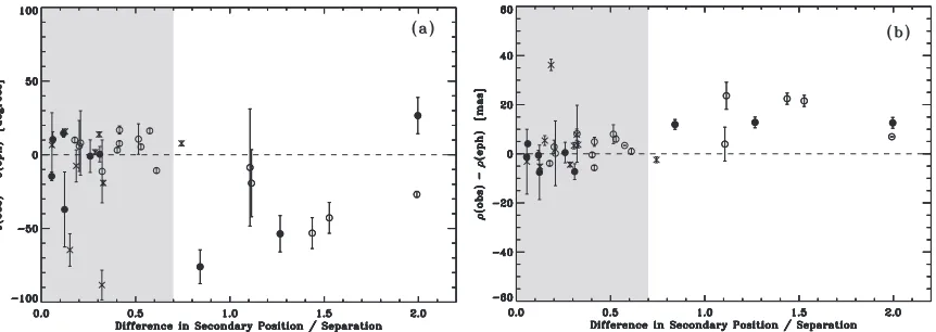
Figure 3.Observed minus ephemeris differences in position angle and separation when comparing the measures presented here with orbital ephemerides of objects having orbital parameters with uncertainties in the Sixth Orbit Catalog of Hartkopf et al. (2001a). Paired observations are treated as two single observations for the purposes of this plot. (a) Position angle residuals and (b) separation residuals. In both plots, filled circles represent the orbits of the highest quality as described in the text, and the error bars are calculated for the observation date based on uncertainties in the orbital parameters appearing in the Sixth Orbit Catalog.
with itself (assuming Gaussian errors). Furthermore, if the astrometry from the two observations is averaged, then this would decrease the sample standard deviation by another factor of√2. Therefore, the best case of the precision value for paired, averaged astrometry is 3.5/2 = 1.8 mas. This is somewhat higher than what we have recently found for observations above the diffraction limit (1.1 mas in Paper II), but given the more challenging nature of sub-diffraction-limited work, still good enough to be quite useful even at very small separations.
2.2. Astrometric Properties
Of the 222 observations initially identified as of interest for this project, 90 are of objects with orbits in the Sixth Catalog of Visual Binary Star Orbits (Hartkopf et al.2001b). If we consider only objects with ephemeris separation below the diffraction limit at the time of observation and having published uncertain-ties in the orbital elements, 66 observations remain. This pro-vides an excellent sample with which to study the measurement accuracy and precision in the sub-diffraction-limited case. We can first study the observed minus ephemeris residuals from the orbits for these measures, treating each measure singly, that is, not pairing any observations, even if two were taken at the same time. This is shown in Figure3. In calculating the ephemeridal uncertaintiesδθandδρin each case from the published uncer-tainties in the orbital elements, we find a large range of values. This highlights the fact that the orbits themselves have a range in quality, but if we consider the highest quality orbits as those with
δθ12◦.0 andδρ 5 mas, then we obtain a mean residual of Δθ= −8.4±5.◦1 with standard deviation ofσΔθ =34.0±3◦.6. For separation, the results areΔρ=+4.5±1.4 mas with stan-dard deviation ofσΔρ=10.2±1.0 mas. The largest residuals in both cases occur at the smallest ephemeris separations, below ∼20 mas. If only observations above this value are considered, then the mean and standard deviations areΔθ= −7.0±3◦.4 and
σΔθ =24.8±2◦.4 for position angle, andΔρ=+0.4±1.2 mas andσΔρ =6.6±0.9 mas in separation. The standard deviation values contain both the uncertainty in the ephemeris and the er-ror, both random and systematic, from our measures. Nonethe-less, these results indicate that it is unwise to report measures below 20 mas because there is at minimum a systematic over-estimate of the separation in these cases. Above this ephemeris separation, on the other hand, there is no evidence for a signifi-cant offset in either coordinate.
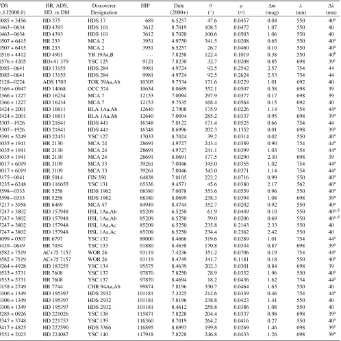
Next, we can pair observations and examine the residuals in this case. We consider three types of pairs: (1) pairs where both observations are taken during the same telescope pointing and are in different filters (sequentially if taken before DSSI was completed in 2008 and simultaneously if taken with DSSI), (2) pre-DSSI pairs that are not taken on the same pointing but are from the same run and are in different filters, and (3) observa-tions taken in the same pointing but in the same filter. These residuals are shown in Figure4, with observation Type 1 drawn as filled circles, observation Type 2 as open circles, and ob-servation Type 3 shown as crosses. The horizontal axis used in these plots is the difference in secondary position between the two observations in arcseconds divided by the mean sepa-ration, which represents a dimensionless consistency parameter characterizing the observation pair. The plots demonstrate that requiring consistency between the two colors (if the observa-tion pair is taken in two filters) does help to distinguish between observations affected by systematic error (most likely residual dispersion) and those that are more trustworthy. On the other hand, the one-filter pairs can have a large residual but a small abscissa, indicating that the color information is indeed neces-sary to make this determination. Note that there will be some duplication in these plots due to cases that can be considered in either Type 2 or Type 3, depending on how the data files for a given run are paired.
Figure4suggests that the following simple approach can be used in the analysis of our sub-diffraction-limited observations:
1. Wherever possible, an observation should be paired with another taken in a different filter. That is, observation Type 1 defined above is most desirable, followed by observation Type 2. For such observation pairs, calculating the difference in secondary position divided by the average separation and applying the data cut at 0.7 will ensure high data quality without significant systematic error.
Figure 4.Observed minus ephemeris differences in position angle and separation when comparing the paired measures presented here with orbital ephemerides of objects having orbital parameters with uncertainties in the Sixth Orbit Catalog of Hartkopf et al. (2001a). The astrometry of both observations has been averaged prior to obtaining the residuals. (a) Position angle residuals and (b) separation residuals. In both plots, filled circles represent paired observations at the same observation date and open circles observations with different observation dates but during the same run. Crosses are observation pairs taken in the same filter. Thex-axis in both cases is the difference in secondary location between the filters divided by the average observed separation. The gray region marks more consistent observation pairs.
the limit of 20 mas); however, it is the only observable available for this purpose.
3. RESULTS
Using the above strategy, we construct two final tables, one which consists of unpaired observations (Table1) and the other which consists of paired observations where the astrometry and observation date (if different between the two observations of the pair) have been averaged (Table2). The majority of measures in the latter table were taken with DSSI. The format for both tables is the same: (1) the Washington Double Star (WDS) number (Mason et al. 2001a), which also gives the right ascension and declination for the object in 2000.0 coordinates; (2) the Bright Star Catalogue (i.e., Harvard Revised, HR) number, or if none, the Aitken Double Star (ADS) Catalogue number, or if none, the Henry Draper Catalogue (HD) number, or if none, the Durchmusterung (DM) number of the object; (3) the Discoverer Designation; (4) theHipparcosCatalogue number (ESA1997); (5) the Besselian date of the observation; (6) the position angle (θ) of the secondary star relative to the primary, with north through east defining the positive sense ofθ; (7) the separation of the two stars (ρ), in arcseconds; (8) the magnitude difference (Δm) of the pair (9) center wavelength of the filter used; and (10) width of the filter in nanometers. Position angles have not been precessed from the dates shown and are left as determined by our analysis procedure, even if inconsistent with previous measures in the literature. Determination of the correct quadrant is extremely challenging for many of the data in these tables due to the small separations and the fact that many systems detected have relatively small magnitude differences, as shown in Figure1(a). This implies that when using these data for orbit determinations, quadrant flips will inevitably be needed at a later stage in some number of cases.
A total of 18 objects in these tables have no previous detection in the 4th Catalog of Interferometric Measures of Binary Stars (Hartkopf et al.2001a); we propose discoverer designations of YSC (Yale-Southern Connecticut) 123-140 here. Thirteen of these objects are known to be spectroscopic binaries from the Geneva–Copenhagen Catalogue or another source, two others are listed as “suspected binaries” in theHipparcosCatalogue, one has no previous indication of binarity in the literature so far as we are aware (HIP 97870=HR 7608), and the remaining
two are first detections of new small-separation components in known binary systems.
3.1. Astrometric Accuracy and Precision
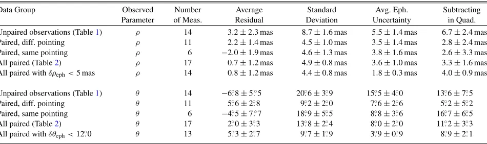
We study the final astrometric accuracy and precision in the same way as described above for the full set of observations, that is, by comparing to the ephemeris position of those objects with orbits in the Sixth Orbit Catalog. We confine our attention to only those orbits which have published uncertainties for the orbital elements, shown in Table3. The astrometric properties of the observations in the two final tables are detailed in Table4 and in Figure 5. In the former, we show the number of measures, average residual (observed minus ephemeris), and standard deviation in both separation and position angle for five subgroups of data: (1) all unpaired observations (i.e., those appearing in Table 1), (2) observations that are paired but which were taken in different telescope pointings, (3) those paired but taken during the same telescope pointing, (4) all paired observations (i.e., those appearing in Table2), and (5) the paired observations of the objects with the highest quality orbits (with ephemeris uncertainty of less than 5 mas in separation or less than 12◦in position angle, respectively. The average residuals of these subsamples show a scatter around 0 of up to∼2σ in the worst case; nonetheless, the sample sizes are not large here and the unpaired observations as well as the sample of all paired observations do not appear to have values that differ significantly from zero. The standard deviations are larger for the unpaired sample than for the all-paired sample; this is at least partly due to the fact that we have averaged the astrometry in the case of the paired observations. However, error from the ephemerides is also included here.
To obtain an estimate of the true measurement uncertainty, we compute the average ephemeris uncertainty and subtract this in quadrature from the standard deviation, in essence assuming that the measurement errors here and those of the orbital elements are uncorrelated. (Since all of the orbits used here have uncertainties in orbital parameters listed in the Sixth Catalog, we can use these to compute uncertainties in the observables
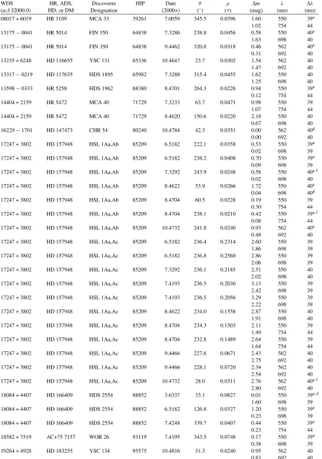
Table 1
Unpaired Double Star Speckle Measures
WDS HR, ADS, Discoverer HIP Date θ ρ Δm λ Δλ
(α,δJ2000.0) HD, or DM Designation (2000+) (◦) () (mag) (nm) (nm)
00085 + 3456 HD 375 HDS 17 689 6.5257 47.6 0.0457 0.04 550 40a
00463−0634 HD 4393 HDS 101 3612 8.7019 108.5 0.0472 1.07 550 40
00463−0634 HD 4393 HDS 101 3612 8.7020 100.6 0.0503 1.06 550 40
00507 + 6415 HR 233 MCA 2 3951 4.9750 341.5 0.0208 0.65 550 40a
00507 + 6415 HR 233 MCA 2 3951 6.5257 26.7 0.0460 0.10 550 40a
00516 + 4412 HD 4901 YR 19Aa,B · · · 7.8258 122.4 0.1019 0.38 550 40b
01576 + 4205 BD+41 379 YSC 125 9121 7.8230 32.7 0.0208 0.85 698 39c
02085−0641 HD 13155 HDS 284 9981 4.9724 92.5 0.2542 2.57 754 44
02085−0641 HD 13155 HDS 284 9981 4.9724 92.5 0.2624 2.53 754 44
02128−0224 ADS 1703 TOK 39Aa,Ab 10305 9.7534 171.6 0.0229 1.01 692 40
02169 + 0947 HD 14068 OCC 574 10634 8.0689 352.1 0.0507 0.58 698 39
02366 + 1227 HD 16234 MCA 7 12153 7.0094 297.9 0.0377 0.17 698 39
02366 + 1227 HD 16234 MCA 7 12153 9.7535 168.4 0.0564 0.15 692 40
02424 + 2001 HD 16811 BLA 1Aa,Ab 12640 2.7908 175.9 0.0226 1.14 754 44a
02424 + 2001 HD 16811 BLA 1Aa,Ab 12640 7.0094 285.2 0.0337 0.95 698 39a
03307−1926 HD 21841 HDS 441 16348 7.0122 171.4 0.0525 0.66 754 44
03307−1926 HD 21841 HDS 441 16348 8.6996 202.3 0.1352 0.01 698 39a
03391 + 5249 HD 22451 YSC 127 17033 8.7024 39.2 0.0314 0.02 550 40a
06035 + 1941 HR 2130 MCA 24 28691 4.9727 243.4 0.0389 0.90 754 44a
06035 + 1941 HR 2130 MCA 24 28691 4.9727 241.1 0.0399 1.03 754 44a
06035 + 1941 HR 2130 MCA 24 28691 8.0691 177.5 0.0290 2.30 698 39
08017 + 6019 HR 3109 MCA 33 39261 7.0046 345.0 0.0355 1.02 754 44a
08017 + 6019 HR 3109 MCA 33 39261 7.0046 343.0 0.0371 1.14 754 44a
13175−0041 HR 5014 FIN 350 64838 7.0105 222.2 0.0716 0.99 550 40a
13235 + 6248 HD 116655 YSC 131 65336 9.4571 45.6 0.0380 2.17 562 40a
13598−0333 HR 5258 HDS 1962 68380 7.0078 353.6 0.0559 0.96 550 40a
13598−0333 HR 5258 HDS 1962 68380 8.0699 238.3 0.0394 1.08 698 39a
17217 + 3958 HR 6469 MCA 47 84949 8.4744 352.7 0.0202 0.92 550 40a
17247 + 3802 HD 157948 HSL 1Aa,Ab 85209 6.5250 61.9 0.0449 0.10 550 40a,d
17247 + 3802 HD 157948 HSL 1Aa,Ab 85209 6.5250 59.0 0.0206 0.69 550 40a,d
17247 + 3802 HD 157948 HSL 1Aa,Ac 85209 6.5250 235.8 0.2143 2.33 550 40
17247 + 3802 HD 157948 HSL 1Aa,Ac 85209 6.5250 234.4 0.2362 2.42 550 40
18099 + 0307 HR 6797 YSC 132 89000 8.4666 319.6 0.0289 1.01 754 44a
18439−0649 HR 7034 YSC 133 91880 8.4638 170.8 0.0344 0.87 698 39a
18582 + 7519 AC+75 7157 WOR 26 93119 7.4236 351.2 0.0706 0.19 754 44a
18582 + 7519 AC+75 7157 WOR 26 93119 8.4749 341.7 0.1181 0.18 550 40a
19264 + 4928 HD 183255 YSC 134 95575 8.4639 202.3 0.0301 0.84 698 39
19533 + 5731 HR 7608 YSC 137 97870 7.8250 28.9 0.0352 1.96 550 40a
19533 + 5731 HR 7608 YSC 137 97870 8.4694 18.2 0.0436 1.62 754 44a
20158 + 2749 HR 7744 CHR 94Aa,Ab 99874 7.8196 330.7 0.0464 1.65 550 40
20306 + 1349 HD 195397 HDS 2932 101181 7.3225 212.6 0.0339 0.46 754 44a
20306 + 1349 HD 195397 HDS 2932 101181 7.8196 238.8 0.0423 1.41 550 40
20306 + 1349 HD 195397 HDS 2932 101181 8.4612 258.8 0.0386 1.08 550 40
23285 + 0926 HD 221026 YSC 138 115871 7.8228 204.4 0.0337 0.98 698 39a
23347 + 3748 HD 221757 YSC 139 116360 8.7019 264.2 0.0416 0.27 550 40a
23417 + 4825 HD 222590 HDS 3366 116895 8.6993 199.8 0.0269 1.46 698 39a
23551 + 2023 HD 224087 YSC 140 117918 7.8228 246.8 0.0433 1.26 698 39a
Notes.
aQuadrant ambiguous.
bThis observation was previously presented in Horch et al. (2010). The data appearing here are the result of a reanalysis using a trinary fit, although the Aa,Ab
component was not of high enough quality to include here.
cThere is some evidence of a very faint third component in this system with separation of 0.45 arcsec. dQuadrant inconsistent with previous measures in the 4th Interferometric Catalog.
pairing observations taken on the same telescope pointing (either sequentially for pre-DSSI observations or simultaneously with DSSI) and those taken on different pointings but during the same observing run. This provides the justification for combining all such pairings into Table2. For the position angle, we find values of 13◦.6 for the unpaired observations and 11◦.2 for the paired observations. These may be converted into an estimate of the linear measurement uncertainty orthogonal to separation
Table 2
Paired Double Star Speckle Measures
WDS HR, ADS, Discoverer HIP Date θ ρ Δm λ Δλ
(α,δJ2000.0) HD, or DM Designation (2000+) (◦) () (mag) (nm) (nm)
00085 + 3456 HD 375 HDS 17 689 7.0106 185.4 0.0547 0.88 550 39
0.71 698 39
00463−0634 HD 4393 HDS 101 3612 10.7172 242.2 0.0290 1.37 562 40
1.44 692 40
00507 + 6415 HR 233 MCA 2 3951 3.5332 310.0 0.0380 0.56 550 39a
1.38 698 39
00507 + 6415 HR 233 MCA 2 3951 7.0106 192.8 0.0461 0.97 550 39
2.64 698 39
00516 + 4412 HD 4901 YSC 123Aa,Ab · · · 8.6911 356.8 0.0165 0.71 562 40
0.25 692 40
00516 + 4412 HD 4901 YSC 123Aa,Ab · · · 10.0044 271.1 0.0307 0.12 562 40
0.04 692 40
00516 + 4412 HD 4901 YSC 123Aa,Ab · · · 10.7144 291.5 0.0154 0.79 562 40
0.55 692 40
00516 + 4412 HD 4901 YR 19Aa,B · · · 8.6911 125.9 0.1004 0.50 562 40b
0.05 692 40b
00516 + 4412 HD 4901 YR 19Aa,B · · · 10.0044 136.4 0.0895 0.17 562 40c
0.56 692 40c
00516 + 4412 HD 4901 YR 19Aa,B · · · 10.7144 132.9 0.0931 0.37 562 40
0.26 692 40
00541 + 6626 HD 5110 YSC 19Aa,Ab 4239 10.7144 224.9 0.0273 1.03 562 40a
0.83 692 40
00541 + 6626 HD 5110 HDS 117Aa,B 4239 3.5332 110.6 0.8551 4.87 550 40
3.74 698 40
00541 + 6626 HD 5110 HDS 117Aa,B 4239 10.7144 108.9 0.8759 3.87 562 40
3.59 692 40
01051 + 1457 ADS 889 YSC 124Aa,Ab 5081 10.7116 89.4 0.0260 0.61 562 40a
0.70 692 40
01057 + 2128 ADS 899 YR 6Aa,Ab 5131 7.0052 17.2 0.0185 1.49 550 39
0.17 754 44
01057 + 2128 ADS 899 YR 6Aa,Ab 5131 10.7116 187.8 0.0358 1.37 562 40a
1.10 692 40d
01101−1425 HD 6978 HDS 153 5475 10.0073 227.6 0.0441 0.91 562 40
0.83 692 40
02085−0641 HD 13155 HDS 284 9981 10.8101 99.5 0.2437 2.95 692 40e
2.96 880 50
02128−0224 ADS 1703 TOK 39 Aa,Ab 10305 10.7117 149.9 0.0374 0.56 562 40
1.16 692 40
02366 + 1227 HD 16234 MCA 7 12153 1.7616 37.4 0.0271 1.64 550 40a,d
0.02 698 40
02366 + 1227 HD 16234 MCA 7 12153 10.7175 123.1 0.0551 0.19 692 40
0.17 880 50
02424 + 2001 HD 16811 BLA 1Aa,Ab 12640 10.7118 312.8 0.0312 0.64 562 40
0.03 692 40
03022−0630 18894 YSC 126 14124 10.0101 153.2 0.0373 1.19 562 40
0.85 692 40
03391 + 5249 HD 22451 YSC 127 17033 10.7147 10.8 0.0411 0.28 562 40
0.30 692 40
03391 + 5249 HD 22451 YSC 127 17033 10.8156 9.5 0.0408 0.33 692 40a
0.18 880 50
03404 + 2957 BD+29 590 HDS 465 17151 10.8100 62.0 0.0417 0.17 692 40a
0.18 880 50d
03496 + 6318 HD 23523 CAR 1 17891 7.8190 61.5 0.0463 0.67 550 40
0.00 698 40
04163 + 3644 HD 26872 YSC 128 19915 10.7202 57.2 0.0318 1.84 562 40a
1.71 692 40
04256 + 1556 HR 1391 FIN 342Aa,Ab 20661 7.8191 212.2 0.0460 0.17 550 40
0.30 698 40
05072−1924 HD 33095 FIN 376 23818 10.8131 237.8 0.0320 0.64 692 40a
0.60 880 50
06416 + 3556 47703 YSC 129 32040 10.8160 269.2 0.0310 0.85 692 40a
0.84 880 50
07338 + 1324 HD 60183 YSC 130 36771 10.8134 119.9 0.0151 0.98 692 40a
Table 2 (Continued)
WDS HR, ADS, Discoverer HIP Date θ ρ Δm λ Δλ
(α,δJ2000.0) HD, or DM Designation (2000+) (◦) () (mag) (nm) (nm)
08017 + 6019 HR 3109 MCA 33 39261 7.0059 345.5 0.0396 1.60 550 39a
1.02 754 44
13175−0041 HR 5014 FIN 350 64838 7.3286 238.8 0.0456 0.58 550 40a
1.63 698 40
13175−0041 HR 5014 FIN 350 64838 9.4462 320.8 0.0318 0.46 562 40a
0.31 692 40
13235 + 6248 HD 116655 YSC 131 65336 10.4647 23.7 0.0302 1.54 562 40
1.47 692 40
13317−0219 HD 117635 HDS 1895 65982 7.3288 315.4 0.0455 1.62 550 40
1.25 698 40
13598−0333 HR 5258 HDS 1962 68380 8.4701 264.3 0.0226 0.94 550 39a
0.12 754 44
14404 + 2159 HR 5472 MCA 40 71729 7.3233 63.7 0.0471 0.98 550 39
1.07 754 44
14404 + 2159 HR 5472 MCA 40 71729 8.4620 150.6 0.0220 2.18 550 40
0.67 698 40
16229−1701 HD 147473 CHR 54 80240 10.4784 42.3 0.0351 0.00 562 40d
0.00 692 40
17247 + 3802 HD 157948 HSL 1Aa,Ab 85209 6.5182 222.1 0.0358 0.53 550 39a
0.02 698 39
17247 + 3802 HD 157948 HSL 1Aa,Ab 85209 6.5182 238.2 0.0408 0.70 550 39a
0.09 698 39
17247 + 3802 HD 157948 HSL 1Aa,Ab 85209 7.3292 243.9 0.0248 0.58 550 40a,f
0.02 698 40
17247 + 3802 HD 157948 HSL 1Aa,Ab 85209 8.4622 53.9 0.0266 1.72 550 40a
0.04 698 40d
17247 + 3802 HD 157948 HSL 1Aa,Ab 85209 8.4704 60.5 0.0228 0.19 550 39
0.30 754 44
17247 + 3802 HD 157948 HSL 1Aa,Ab 85209 8.4704 238.1 0.0210 0.42 550 39a,f
0.08 754 44
17247 + 3802 HD 157948 HSL 1Aa,Ab 85209 10.4732 241.8 0.0240 0.93 562 40a
0.48 692 40
17247 + 3802 HD 157948 HSL 1Aa,Ac 85209 6.5182 236.4 0.2314 2.60 550 39
1.86 698 39
17247 + 3802 HD 157948 HSL 1Aa,Ac 85209 6.5182 236.8 0.2560 2.86 550 39
2.06 698 39
17247 + 3802 HD 157948 HSL 1Aa,Ac 85209 7.3292 236.1 0.2185 2.51 550 40
2.02 698 40
17247 + 3802 HD 157948 HSL 1Aa,Ac 85209 7.4193 236.5 0.2030 3.13 550 39
2.42 698 39
17247 + 3802 HD 157948 HSL 1Aa,Ac 85209 7.4193 236.5 0.2056 3.29 550 39
2.22 698 39
17247 + 3802 HD 157948 HSL 1Aa,Ac 85209 8.4622 234.0 0.1558 2.87 550 40
1.91 698 40
17247 + 3802 HD 157948 HSL 1Aa,Ac 85209 8.4704 234.3 0.1503 2.11 550 39
1.49 754 44
17247 + 3802 HD 157948 HSL 1Aa,Ac 85209 8.4704 232.8 0.1489 2.64 550 39
1.64 754 44
17247 + 3802 HD 157948 HSL 1Aa,Ac 85209 9.4466 227.6 0.0671 2.43 562 40
2.75 692 40
17247 + 3802 HD 157948 HSL 1Aa,Ac 85209 9.4466 228.1 0.0720 2.34 562 40
2.54 692 40
17247 + 3802 HD 157948 HSL 1Aa,Ac 85209 10.4732 28.0 0.0311 2.76 562 40a,f
2.80 692 40
18084 + 4407 HD 166409 HDS 2554 88852 3.6337 33.1 0.0827 0.01 550 39a,d
1.60 698 39
18084 + 4407 HD 166409 HDS 2554 88852 6.5182 126.8 0.0327 1.20 550 39a
0.23 698 39
18084 + 4407 HD 166409 HDS 2554 88852 7.4248 339.7 0.0407 0.44 550 39a
0.23 754 44
18582 + 7519 AC+75 7157 WOR 26 93119 7.4195 343.5 0.0748 0.17 550 39a
0.38 698 39
19264 + 4928 HD 183255 YSC 134 95575 10.4816 51.3 0.0240 0.95 562 40
Table 2 (Continued)
WDS HR, ADS, Discoverer HIP Date θ ρ Δm λ Δλ
(α,δJ2000.0) HD, or DM Designation (2000+) (◦) () (mag) (nm) (nm)
19380 + 3354 BD+33 3529 YSC 135Aa,Ab 96576 10.4816 133.0 0.0254 0.51 562 40a
0.50 692 40
19467 + 4421 HD 187160 YSC 136 97321 10.4737 322.8 0.0336 1.28 562 40
1.18 692 40
19533 + 5731 HR 7608 YSC 137 97870 10.4816 340.7 0.0300 1.43 562 40
1.64 692 40
19533 + 5731 HR 7608 YSC 137 97870 10.4817 328.5 0.0290 1.49 562 40
1.76 692 40
20329 + 4154 HD 195987 BLA 8 101382 7.8183 295.5 0.0062 1.75 550 39a
0.47 754 44
22087 + 4545 HR 8448 YSC 15 109303 10.4819 344.6 0.0295 1.12 562 40a
1.68 692 40
23049 + 0753 HD 218055 YR 31 113974 7.8214 359.5 0.0267 0.46 550 40
1.64 698 40
23347 + 3748 HD 221757 YSC 139 116360 10.7197 272.5 0.0330 0.64 562 40a
0.49 692 40
23417 + 4825 HD 222590 HDS 3366 116895 10.7198 252.8 0.0191 0.06 562 40a
1.68 692 40d
Notes.
aQuadrant ambiguous.
bThis observation was previously presented in Paper I. The data presented here are the result of a reanalysis using a trinary fit to include the
small separation component YR 123Aa,Ab.
cIn the course of reanalyzing this observation to include the small separation component YR 123Aa,Ab, it was noticed that the magnitude
differences appearing in Paper II for the two filters shown were reversed. The values appearing here correct that error.
dThe observation in this filter had a quadrant inconsistent with the other observation and was flipped prior to averaging the two position angle
values.
ePossible sub-diffraction-limited component, but the astrometry is not consistent between the two observations. fQuadrant inconsistent with previous measures in the 4th Interferometric Catalog.
Table 3
Orbits Used for the Final Measurement Precision Study WDS Discoverer Designation HIP Grade Orbit Reference
00507 + 6415 MCA 2 3951 3 Mason et al.1997
01057 + 2128 YR 6Aa,Ab 5131 3 Horch et al.2011
02366 + 1227 MCA 7 12153 2 Mason1997
02424 + 2001 BLA 1Aa,Ab 12640 2 Mason1997
06416 + 3556 YSC 129 32040 9 Ren & Fu2010a 08017 + 6019 MCA 33 39261 3 Balega et al.2004 13175−0041 FIN 350 64838 2 Hartkopf et al.1996 17247 + 3802 HSL 1Aa,Ab 85209 3 Horch et al.2006b 20329 + 4154 BLA 8 101382 8 Torres et al.2002b
23347 + 3748 YSC 139 116360 9 Ren & Fu2010a
Notes.
aNo measures of these objects appear in the 4th Interferometric Catalog, but an
orbit has been obtained by fitting revisedHipparcosintermediate astrometric data.
bOnly two successful measures of this object appear in the 4th Interferometric
Catalog, but an orbit has been obtained with long baseline optical interferometry.
4.6 mas. Recalling that the measures in Table2are the average of those obtained in two filters, we would expect the difference in precision to be a factor of √2 between the two samples; indeed, 7.2/√2 =5.1 mas, very similar to 4.6 mas. However, it is important to emphasize that the paired observations also represent a sample that includes separations at and below 0.25 of the diffraction limit, while the unpaired sample is limited to somewhat larger separations.
To give a feel for the data used in this study, we show three of the orbits used in the study in Figures6and7. In Figure6(a), we
plot existing and new data for YR 6Aa,Ab together with our own recent orbit determination (Paper II). The new data presented here fall very close to the predicted orbital path, although it should be stated that all data to date has been reported by our group, and a greater diversity of observers would be desirable in order to make certain that no systematic trends exist. Figure6(b) shows the orbital data of BLA 1Aa,Ab, where the orbit is that of mason (1997). In this case, there is more scatter in the orbital points most likely owing to the contributions of several observers, but again, despite the small scale of the orbit by speckle standards, the data quality of the points presented here is reasonably good.
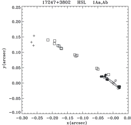
In Figure 7, we show the multiple system HIP 85209 = HD 157948. This is a hierarchical quadruple system, where the widest component (COU 1142) has a separation of approx-imately 2 arcsec and is not shown. (This component has shown little motion over the last 20 years according to data in 4th Interferometric Catalog.) However, the innermost pair, a spec-troscopic binary whose orbit was determined by Latham et al. (1992) and updated by Goldberg et al. (2002), was resolved and measured several times by Horch et al. (2006b) using the Fine Guidance Sensors (FGSs) on theHubble Space Telescope. The FGS observations also revealed the presence of an intermediate-separation component (HSL 1Aa,Ac) that has been easily mon-itored with speckle observations at WIYN over the past few years. This component has a number of measures in Tables1
[image:9.612.44.296.428.550.2]Figure 5.Observed minus ephemeris differences in position angle and separation when comparing the measures presented here with orbital ephemerides of objects having orbital parameters with uncertainties in the Sixth Orbit Catalog of Hartkopf et al. (2001a). Paired observations taken in the same telescope pointing are shown as filled circles, paired observations taken in different pointings are shown as open circles, and unpaired observations are shown as crosses. Paired observations are subject to the data cut diff/sep<0.7, and unpaired observations subject to observed separation>0.02 arcsec. (a) Position angle residuals and (b) separation residuals.
Figure 6.Two examples of objects in Tables1and2with orbits. (a) The orbit of Horch et al.2011for YR 6Aa,Ab=HIP 5131=HR 310 together with data from the literature and our measures from Table2. The latter are shown with filled circles. (b) The orbit of mason (1997) for BLA 1Aa,Ab=HIP 12640=HD 16811 together with our measures from Tables1and2. The latter are shown with filled circles. In both plots, all points are drawn with line segments from the data point to the location of the ephemeris prediction on the orbital path. North is down and east is to the right.
Table 4
Measurement Precision Results
Data Group Observed Number Average Standard Avg. Eph. Subtracting
Parameter of Meas. Residual Deviation Uncertainty in Quad.
Unpaired observations (Table1) ρ 14 3.2±2.3 mas 8.7±1.6 mas 5.5±1.4 mas 6.7±2.4 mas
Paired, diff. pointing ρ 11 2.2±1.4 mas 4.5±1.0 mas 3.5±1.4 mas 2.8±2.4 mas
Paired, same pointing ρ 6 −2.0±1.9 mas 4.6±1.3 mas 3.8±1.6 mas 2.6±3.3 mas
All paired (Table2) ρ 17 0.7±1.2 mas 4.9±0.8 mas 3.6±1.0 mas 3.3±1.6 mas
All paired withδρeph<5 mas ρ 14 0.8±1.2 mas 4.4±0.8 mas 1.8±0.3 mas 4.0±0.9 mas
Unpaired observations (Table1) θ 14 −6.◦8±5.◦5 20.◦6±3.◦9 15.◦5±4.◦0 13.◦6±7.◦5 Paired, diff. pointing θ 11 5.◦6±2.◦8 9.◦2±2.◦0 7.◦6±2.◦6 5.◦2±5.◦2 Paired, same pointing θ 6 −4.◦5±7.◦7 18.◦9±5.◦5 8.◦8±3.◦6 16.◦7±6.◦5 All paired (Table2) θ 17 2.◦0±3.◦3 13.◦8±2.◦4 8.◦0±2.◦0 11.◦2±3.◦3 All paired withδθeph<12.◦0 θ 13 5.◦3±2.◦7 9.◦7±1.◦9 3.◦9±0.◦9 8.◦9±2.◦1
hand end with the 2010 sub-diffraction-limited measure appear-ing in Table2. This measure and the one for the spectroscopic pair of the same observation date were obtained with a triple-star fit to the power spectrum resulting in the two sub-diffraction-limited separations (with the fourth component just off of the
[image:10.612.70.545.536.677.2]Table 5 Two Orbit Refinements
Object HIP P a i Ω T0 e ω
(yr) (mas) (◦) (◦) (yr) (◦)
FIN 350 64838 9.165 80.8 55.6 201.6 2008.39 0.632 346.8
±0.010 ±1.4 ±2.2 ±1.2 ±0.04 ±0.014 ±2.3 MCA 40 71729 9.151 71.0 107.4 79.0 2003.66 0.049 265.
±0.041 ±0.6 ±0.6 ±0.6 ±0.28 ±0.021 ±13.
case, the best approach for this system would be to incorporate all of the data available for the system in a simultaneous orbit fit for both HSL 1Aa,Ac and the inner pair. We hope that the data presented here will encourage other observers to work on this system over the next few years.
3.2. Photometric Accuracy and Precision
Our standard method for estimating the accuracy and preci-sion of our differential photometry in previous papers has been to compare with the space-based magnitude differences appear-ing in theHipparcosCatalogue. We have generally considered only speckle observations taken in a filter with properties sim-ilar to theHpfilter. However, for objects presented here, there
are few that have values listed in the Catalogue, owing to their generally very small separations. Those that were measured by
Hipparcoshave large uncertainties in ΔHp, typically 0.2 mag or more, much worse than typical forHipparcosdata. Nonethe-less, with the sample for which the comparison can be made (12 objects from the paired sample, and 4 from the unpaired), we find observed minusHipparcosresiduals that differ from zero by less than 1σ in both cases, and standard deviations in the 0.4–0.5 magnitude range. However, the mean error of theΔHp values in both cases is also in the same range. Therefore, we conclude that the measurement error inΔmfor sub-diffraction-limited measures is certainly much lower than 0.4 mag, and that there is no evidence at this time that it is significantly larger than what we have previously reported for WIYN speckle data above the diffraction limit, roughly 0.1 mag per observation.
4. ORBIT DETERMINATIONS
4.1. Two Orbit Refinements
In Table5, we show new orbital elements for two systems for which the observations presented here, together with other relatively recent observations in the 4th Interferometric Cata-log, permit modest orbit revisions. To calculate the orbital ele-ments, we have used our own orbit fitting routine, described in MacKnight & Horch (2004). We do not anticipate that these orbits are dramatically better in quality than those published earlier; nonetheless, since they are small-separation systems, the data used span a more complete range in position an-gle and provide an up-to-date dynamical picture prior to dis-cussing the evolutionary status of the components of these systems.
[image:11.612.44.296.68.142.2]The first of these binaries is FIN 350(= HIP 64838 = HR 5014), where the previous orbit (which is Grade 2) was computed by Hartkopf et al. (1996). Since that time, several observations have appeared in the literature, including our mea-sures presented here. Our orbit increases both the semi-major axis and the period slightly while decreasing the uncertain-ties of both substantially. The total mass, when computed with the revisedHipparcosparallax (van Leeuwen2007), therefore changes from 3.3±3.0M to 3.4±0.3M. Given that this
Figure 7.Orbital data for HSL 1=HIP 85209. For the inner pair, measures appearing the 4th Interferometric Catalog are shown as open circles, and measures from Tables1and2are shown as filled circles. The orbit plotted is that of Horch et al. (2006b). For the outer component, measures in the 4th Interferometric Catalog are shown as pluses, and the measures from Tables1 and2are shown as squares. North is down and east is to the right.
is an F0V system with at most a small magnitude difference, a total mass of approximately 3.0–3.2Mis expected from the photometry, in excellent agreement with the current orbit. To make the conversion from spectral type to stellar mass, we have used a standard table from the literature (Schmidt-Kaler1982). For MCA 40(= HIP 71729 = HD 129132 = HR 5472), the orbit currently listed in the Sixth Catalog is also Grade 2, that of Baize (1989), which we improve upon here at least by estimating uncertainties for the elements. From these we can deduce a total mass of 6.7 ±1.4M. However, the spectral type in SIMBAD7 is listed as G0V difficult to reconcile with this result. The absolute magnitude derived from an apparent magnitude of 6.23 and revised Hipparcosparallax of 8.60± 0.61 mas is +0.83, much too bright for a G-type dwarf pair. (An extinction estimate, though less than 0.1 mag, was included using the NASA/IPAC reddening and extinction map available on the IPAC Web site.8) We suggest therefore that at least the primary is evolved and, given the fact that the magnitude differences observed to date are not terribly large (though with considerable scatter), it may be that both components have left the main sequence. If so, this system could provide quite a sensitive test of stellar evolution theory with more high-quality differential photometry. Graphical representations of our orbits for both FIN 350 and MCA 40 are shown in Figure8.
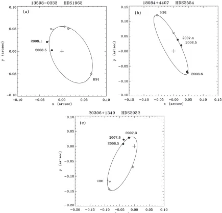
4.2. Three Preliminary Orbits
With the astrometric data in hand from Tables 1 and 2
and in the literature, it is possible to calculate first orbits for three objects, with the caveat that more data will clearly be needed to make the elements definitive. These are shown in Figure9. However, these orbits, together with photometric and spectroscopic information, permit a useful discussion of the status of these systems at present. The orbital elements we derive are shown in Table6, and the astrometric data and residuals are
7 http://simbad.u-strasbg.fr/simbad
Figure 8.Orbit refinements calculated here for (a) FIN 350=HIP 64838 and (b) MCA 40=HIP 71729. Measures appearing the 4th Interferometric Catalog are shown as open circles, and measures from Tables1and2are shown as filled circles. All points are drawn with line segments from the data point to the location of the ephemeris prediction on the orbital path. The current orbit in the Sixth Catalog is shown as a dashed line. North is down and east is to the right.
[image:12.612.88.523.306.722.2]Table 6 Three Preliminary Orbits
Object HIP P a i Ω T0 e ω
(yr) (mas) (◦) (◦) (yr) (◦) HDS 1962 68380 10.7 72.7 54. 204. 2008.29 0.413 60.
±0.5 ±5.5 ±4. ±4. ±0.21 ±0.027 ±10. HDS 2554 88852 21.6 111.8 75.3 208.3 2001.4 0.217 160.
±0.7 ±3.1 ±1.7 ±1.7 ±0.7 ±0.033 ±12. HDS 2932 101181 26.1 122.4 66.9 170.5 2006.12 0.829 309.5
±0.6 ±3.9 ±1.6 ±2.0 ±0.09 ±0.011 ±2.5
shown in Table7. Here again we have used the fitting routine of MacKnight & Horch (2004).
The first of these systems is HDS 1962(= HIP 68380 = HD 122106). Although the latest version of the Geneva–Copenhagen Catalogue (Holmberg et al.2009) gives the iron abundance of this system as slightly metal-rich, [Fe/H] =+0.13, it does not give a mass ratio. There is a non-detection at 1988.163 by McAlister et al. (1993) for which our orbital elements predict a separation of 52.5 mas. This may be an indi-cation that the data to date produce a period that is slightly too large. If we compute the ephemeris position with P =
10.2 years (1σ lower that the value presented), then the sep-aration is 26 mas, well below the stated limit of the observation of 38 mas. Nonetheless, combining the period and semi-major axis obtained here with the revisedHipparcosparallax of van Leeuwen (2007), the mass sum is 1.6±0.5M. On the other hand, this system has spectral type of F8V in the SIMBAD database, but the absolute magnitude that we calculate from the apparent magnitude, parallax, and extinction (again from the NASA/IPAC online map) is +1.8, too bright by over 1.5 mag to be explained by a pair on the main sequence with that spectral type. The speckle andHipparcosmagnitude differences
avail-able in the 4th Interferometric Catalog suggest a value near 1 inV, so perhaps an F7IV–F8V pair comes closer to matching the photometry here. If so, this suggests a mass sum of perhaps 2.5M, somewhat higher than that obtained from the orbit, but within 2σ. If the true value of the period is lower than that of our orbit as the McAlister non-detection suggests, this would of course increase the mass sum, making it more consistent with the 2.5Mvalue.
The second orbit we present is that of HDS 2554(= HIP 88852 = HD 166409). The Hipparcos data point is in the third quadrant, and subsequent observations have been in the first and second quadrants, thus the position angles available now cover nearly a full orbit since the discovery observation in 1991. This object is slightly below the solar abundance ([Fe/H] = −0.10 according to Holmberg et al. 2009), and once again no mass fraction appears in the Geneva–Copenhagen Catalogue. The system has spectral type F5 in SIMBAD, and the differential photometry that exists at present supports a modest magnitude difference, approximately 0.5 mag. The implied absolute magnitude using the revised Hipparcos parallax is +1.6, which is approximately a magnitude too bright for a main-sequence pair and would seem to suggest that the primary may be slightly evolved. If it is composed of an F(4–5)IV primary and an F(7–8)V secondary, then this implies a total mass in the range of perhaps 2.6–3.0M, whereas the orbital elements in combination with the same parallax value give 3.1±0.5M.
Finally, we have the case of HDS 2932(= HIP 101181= HD 195397), a system with spectral type F8. Of the three systems discussed here, this is the most metal-poor, with [Fe/H] = −0.17, and the mass fraction in the Geneva– Copenhagen Catalogue ism2/m1 =0.578±0.037. The
mag-nitude difference appears to be approximately 1, given four measures in the 4th Interferometric Catalog; however, the Hip-parcosmeasure has a large uncertainty and there is significant
Table 7
Orbital Data and Residuals for the Objects in Table6
Object HIP Date θ ρ Δθ Δρ Reference
(Bess. Yr.) (◦) () (◦) (mas)
HDS 1962 68380 1988.163 . . . <0.038 [2.2] [52.5]a McAlister et al.1993
1991.25 53. 0.083 −0.3 1.7 ESA1997
2006.1943 163.7 0.052 3.7 2.5 Mason et al.2009
2007.0078 173.6b 0.0559 −12.1 0.0 This paper
2007.4174 206.4 0.055 7.0 3.3 Horch et al.2010
2008.0699 238.3 0.0394 7.3 2.3 This paper
2008.4701 264.3 0.0226 −6.1 −4.9 This paper
HDS 2554 88852 1991.25 205. 0.132 0.1 −0.3 ESA1997
2002.3229 33.5 0.087 4.2 −1.7 Horch et al.2008
2003.6337 33.1 0.0827 −5.5 3.6 This paper
2006.5182 126.8 0.0327 9.7 2.9 This paper
2007.4248 159.7b 0.0407 −0.7 −0.2 This paper
2008.4665 180.1 0.061 −1.5 −2.8 Horch et al.2010
HDS 2932 101181 1991.25 325. 0.144 3.53 −1.8 ESA1997
1997.7227 329.6 0.167 −3.22 5.8 Mason et al.1999
1998.7058 . . . <0.054 [330.5] [163.5]a Mason et al.2001b
2004.8260 356.5 0.070 3.2 1.8 Balega et al.2007
2007.3225 212.6 0.0339 −4.7 −0.2 This paper
2007.8196 238.8 0.0423 1.8 6.8 This paper
2008.4612 258.8 0.0385 1.4 −2.5 This paper
Notes.
aThe numbers shown in brackets are the ephemeris values obtained from our orbital elements, therefore indicating the expected position angle
and separation for these non-detections.
bThe quadrant of this observation has been flipped here relative to that appearing in Table1or 2 to make a more sensible sequence in position
[image:13.612.80.536.464.695.2]variation in the three remaining measures. The absolute magni-tude derived from the apparent magnimagni-tude and revised Hippar-cosresult is relatively consistent with a main-sequence or near-main-sequence system, so allowing for a sizeable range in sec-ondary spectral type due to the uncertainty in the magnitude dif-ference, perhaps we have an F(6–8)V primary with a G(1–6)V. This implies masses of∼1.26±0.10Mand 0.96±0.06M, so that is a mass ratio of 0.76±0.07. While the mass ratio is larger than that in the Geneva–Copenhagen Catalogue, the total mass agrees quite well with that obtained from our orbital parameters in Table6and the parallax, namely 2.0±0.5M. One aspect of the analysis here is difficult to explain: the non-detection by mason et al. in 1998, even though the same group did suc-cessfully resolve the system about a year before. We explored orbits which place the secondary below the diffraction limit at their observation date, but this reduces the period significantly, and in view of the photometry and the distance information available, unrealistically. Several of our own measures of this system taken over the past few years were judged to be too poor in quality to report, so more work will be needed to fully understand the nature of this difficulty.
5. CONCLUSIONS
We have analyzed a significant sample of sub-diffraction-limited measures of binary stars taken at the WIYN 3.5 m Telescope over the last several years. These data show that, under certain conditions, it is possible to obtain high-quality measures at separations below 0.25 of the diffraction limit. Sub-diffraction-limited speckle observations are however successful for a smaller range of magnitude differences and only for brighter targets compared with those above the diffraction limit. It is important to guard against a systematic overestimate of separation in working below the diffraction limit; a reasonably simple and effective way to do this is to take data of the target in two colors and to require consistency in the position of the secondary in both observations. One may also then average the astrometry obtained to reduce random error. Following this strat-egy leads to results that show no evidence of systematic error and have repeatability of approximately 2 mas. Overall mea-surement precision for the sample presented here is somewhat higher, approximately 3.3–4.0 mas, but may be attributed to the use of different instrumentation and observing conditions over the years. If two observations in different filters are not available, we find that it is unwise to report separations below approxi-mately 0.5 of the diffraction limit since the systematic overes-timate in separation which is most prominent at the smallest separations. We report 47 measures of this type where the lin-ear measurement uncertainty is estimated to be approximately 7 mas.
Modest orbit revisions for two systems are reported; the uncertainties for the orbital elements reported here are small enough to permit a brief report on the evolutionary status of these systems. FIN 350 appears to consist of a late-F + early-G main-sequence system, whereas the data of MCA 40 on balance support an evolved primary and possibly an evolved secondary. New orbits are reported for three Hipparcos double stars. A combination of the orbital information and photometry results in a sensible picture for main-sequence components for HDS 2932, while HDS 1962 and HDS 2554 may have primary stars that have evolved off of the main sequence.
We thank the Kepler Science Office located at the NASA Ames Research Center for providing partial financial support for the upgraded DSSI instrument. It is also a pleasure to thank all of the outstanding staff at WIYN for their assistance and support over the years. This work was funded by NSF Grant AST-0908125. It made use of the Washington Double Star Catalog maintained at the U.S. Naval Observatory and the SIMBAD database, operated at CDS, Strasbourg, France.
REFERENCES
Baize, P. 1989, A&AS,81, 415
Balega, I. I., Balega, Y. Y., Maksimov, A. F., Malogolovets, E. V., Rastegaev, D. A., Shkhagosheva, Z. U., & Weigelt, G. 2007, Astrophys. Bull.,62, 339
Balega, I. I., Balega, Y. Y., & Malogolovets, E. V. 2004, in IAU Symp. 224, The A-Star Puzzle, ed. J. Zverko, J. Ziznovsky, S. J. Adelman, & W. W. Weiss (Cambridge: Cambridge Univ. Press),683
Docobo, J. A., Tamazian, V. S., Balega, Y. Y., & Melikian, N. D. 2010,AJ,140, 1078
ESA 1997, TheHipparcosandTychoCatalogues (ESA SP 1200; Noordwijk: ESA)
Goldberg, D., Mazeh, T., Latham, D. W., Stefanik, R. P., Carney, B. W., & Laird, J. B. 2002,AJ,124, 1132
Hartkopf, W. I., Mason, B. D., & McAlister, H. A. 1996,AJ,111, 370 Hartkopf, W. I., Mason, B. D., & Worley, C. E. 2001a,AJ,122, 3472(see also
http://www.usno.navy.mil/USNO/astrometry/optical-IR-prod/wds/orb6) Hartkopf, W. I., McAlister, H. A., & Mason, B. D. 2001b,AJ,122, 3480 (see
alsohttp://www.usno.navy.mil/USNO/astrometry/optical-IR-prod/wds/int4) Holmberg, J., Nordstr¨om, B., & Andersen, J. 2009,A&A,501, 941
Horch, E. P., Falta, D., Anderson, L. M., DeSousa, M. D., Miniter, C. M., Ahmed, T., & van Altena, W. F. 2010,AJ,139, 205
Horch, E. P., Franz, O. G., & van Altena, W. F. 2006a,AJ,132, 2478 Horch, E. P., Franz, O. G., Wasserman, L. H., & Heasley, J. N. 2006b,AJ,132,
836
Horch, E. P., Gomez, S. C., Sherry, W. H., Howell, S. B., Anderson, L. M., Ciardi, D. R., & van Altena, W. F. 2011,AJ,141, 45(Paper II)
Horch, E. P., Meyer, R. D., & van Altena, W. F. 2004,AJ,127, 1727 Horch, E. P., Ninkov, Z., van Altena, W. F., Meyer, R. D., Girard, T. M., &
Timothy, J. G. 1999,AJ,117, 548
Horch, E. P., Robinson, S. E., Meyer, R. D., van Altena, W. F., Ninkov, Z., & Piterman, A. 2002,AJ,123, 3442
Horch, E. P., van Altena, W. F., Cyr, W. M., Kinsman-Smith, L., Srivastava, A., & Zhou, J. 2008,AJ,136, 312
Horch, E. P., Veillette, D. R., Baena Gall´e, R., Shah, S. C., O’Rielly, G. V., & van Altena, W. F. 2009,AJ,137, 5057(Paper I)
Latham, D. W., et al. 1992,AJ,104, 774
MacKnight, M., & Horch, E. P. 2004, BAAS,36, 788 Mason, B. D. 1997,AJ,114, 808
Mason, B. D., Hartkopf, W. I., Gies, D. R., Henry, T. J., & Helsel, J. W. 2009,AJ, 137, 3358
Mason, B. D., Hartkopf, W. I., Holdenried, E. R., & Rafferty, T. J. 2001a,AJ, 121, 3224
Mason, B. D., McAlister, H. A., Hartkopf, W. I., Griffin, R. F., & Griffin, R. E. M. 1997,AJ,114, 1607
Mason, B. D., Wycoff, G. L., Hartkopf, W. I., Douglass, G. G., & Worley, C. E. 2001b,AJ,122, 3466(see alsohttp://www.usno.navy.mil/USNO/astrometry /optical-IR-prod/wds/WDS)
Mason, B. D., et al. 1999,AJ,117, 1890
McAlister, H. A., Mason, B. D., & Hartkopf, W. I. 1993,AJ,106, 1639 Meyer, R. D., Horch, E. P., Ninkov, Z., van Altena, W. F., & Rothkopf, C. A.
2006,PASP,118, 162
Nordstr¨om, B., et al. 2004,A&A, 419, 989 Ren, S., & Fu, Y. 2010,AJ,139, 1975
Schmidt-Kaler, T. 1982, in Stars and Star Clusters, ed. K. Schaefers & H.-H. Voigt (Landolt–B¨ornstein New Series, Group 6, Vol. 2b; Berlin: Springer), 1 Tokovinin, A. A. 1985, A&AS,61, 483
Tokovinin, A. A., Mason, B. D., & Hartkopf, W. I. 2010,AJ,139, 743 Torres, G., Boden, A. F., Latham, D. W., Pan, W., & Stefanik, R. P. 2002,AJ,
124, 1716