Graph Embedding Using Frequency Filtering

(1)

This is a repository copy of

Graph Embedding Using Frequency Filtering

.

White Rose Research Online URL for this paper:

http://eprints.whiterose.ac.uk/148585/

Version: Accepted Version

Article:

Bahonar, Hoda, Mirzaei, Abdolreza, Sadri, Saeed et al. (1 more author) (Accepted: 2019)

Graph Embedding Using Frequency Filtering. IEEE Transactions on Pattern Analysis and

Machine Intelligence. ISSN 0162-8828 (In Press)

[email protected] https://eprints.whiterose.ac.uk/

Reuse

Items deposited in White Rose Research Online are protected by copyright, with all rights reserved unless indicated otherwise. They may be downloaded and/or printed for private study, or other acts as permitted by national copyright laws. The publisher or other rights holders may allow further reproduction and re-use of the full text version. This is indicated by the licence information on the White Rose Research Online record for the item.

Takedown

If you consider content in White Rose Research Online to be in breach of UK law, please notify us by

(2)

Graph Embedding Using Frequency Filtering

Hoda Bahonar, Abdolreza Mirzaei, Saeed Sadri, Richard C. Wilson

, Senior Member, IEEE

Abstract—The target of graph embedding is to embed graphs in vector space such that the embedded feature vectors follow the differences and similarities of the source graphs. In this paper, a novel method named Frequency Filtering Embedding (FFE) is proposed which uses graph Fourier transform and Frequency filtering as a graph Fourier domain operator for graph feature extraction. Frequency filtering amplifies or attenuates selected frequencies using appropriate filter functions. Here, heat, anti-heat, part-sine and identity filter sets are proposed as the filter functions. A generalized version of FFE named GeFFE is also proposed by defining pseudo-Fourier operators. This method can be considered as a general framework for formulating some previously defined invariants in other works by choosing a suitable filter bank and defining suitable pseudo-Fourier operators. This flexibility empowers GeFFE to adapt itself to the properties of each graph dataset unlike the previous spectral embedding methods and leads to superior classification accuracy relative to the others. Utilizing the proposed part-sine filter set which its members filter different parts of the spectrum in turn improves the classification accuracy of GeFFE method. Additionally, GeFFE resolves the cospectrality problem entirely in tested datasets.

Index Terms—Spectral graph embedding, graph Fourier transform, heat kernel, frequency filtering, graph classification

F

1 I

NTRODUCTION

T

HE key issue in pattern recognition is the formal defi-nition of pattern space, which is able to represent all dis-criminative information among different objects. The clas-sical statistical pattern recognition follows this goal using vectors as the object representation formalism. There exists a wide range of well-defined operators and well-developed efficient algorithms in this approach [1], [2]. Nevertheless, the nature of patterns in some cases such as bioinformatics and chemistry [3], document analysis [4], network traffic control [5] and images classification [6] are not only de-pendent on features, but also structural relations between them. In these situations, graphs are versatile alternatives to feature vectors. However, graphs are not intrinsically vectorial, which leads to increased complexity of many al-gorithms in the graph domain. For example, comparison of two vectors is done in linear time, while comparison of two graphs (graph isomorphism) has exponential complexity. This behavior is observed because, unlike the samples of a vector, there is no standard ordering for the nodes and edges in a graph. Similarly, it is non-trivial to define some basic operators required for many algorithms such as sum and product in the context of graphs. So only a few pattern recognition algorithms which are usually based on distance and its derivatives have direct counterparts in the graph domain [7], [8], [9]. The graph algorithms of this type come from a classical period of graph based pattern recognition [8]. In the modern period, two major approaches have been followed for making use of the powerful existing algorithms of statistical pattern recognition, namely kernel-based meth-ods and embedding methmeth-ods. Kernel-based methmeth-ods re-place dot product with a graph kernel in algorithms which

• H. Bahonar, A. Mirzaei and S. Sadri are with the Department of Electrical and Computer Engineering, Isfahan University of Technology, Isfahan 84156-83111, Iran.

E-mail: [email protected], [email protected], [email protected]

• R. C. Wilson is with Department of Computer Science, University of York, UK.

E-mail: [email protected]

are formulated in terms of dot products [10], [11], [12]. Graph embedding methods extract structural features from graph and put them together in a vector format to make use of algorithms which process and analyze feature vectors di-rectly [13], [14]. So graph embedding offers an easy solution for machine learning problems using the power of graphs as symbolic data structures and computational advantage of feature vectors. Two main requirements of embedded feature vectors are that they are invariant and informative. Being invariant means that the embedded vectors should be the same for every selected node/edge ordering. These vec-tors should be informative as well, i.e. they should contain enough discriminative features such that similar structures are close together and different structures are far away from each other in the embedding space [14].

Employing graph spectra is a natural way for extracting invariants in an acceptable time. There are a variety of methods in this area [6], [14], [15], [16], [17], [18]. The ques-tion is if the feature vectors extracted by these methods are informative enough to have good performance in different applications. The discriminative structures vary from one application to another. In some applications, the features based on small scale connectivity perform better, while the large-scale structures are better candidates for others [19]. The cycles, paths, and loops have different importance in recognizing the patterns of different graph sets [17]. So for the embedding method being universal, it should be flexible enough to represent any type of graph similarities. This flexibility is not observed in previous embedding methods as their properties are the same regardless of the application in hand.

(3)

features.

Fourier analysis provides better understanding of the signal by transferring it to another domain [21]. This behavior is very useful while important features are not easily discover-able in the original domain [22], [23], [24]. For example, one way for edge detection is to locally search within the image to find a sharp change in the brightness of the pixels. How-ever this operation needs scanning all the pixels to compare the brightness of them and their neighbors. Fourier analysis makes this approach easier by filtering the high frequencies. In other words, edge features of original domain spread all over the image, but when these features are transformed into the Fourier domain, their information is limited to a narrow range of frequency values. More generally, Fourier analysis creates a kind of scale-space representation, with small-scale features represented in the high frequencies and large-scale structure in the low frequencies.

Similarly, the key information in graphs appears at different scales (i.e. frequencies) in different applications. For exam-ple when predicting the domain of a protein graph, the large-scale organization of the protein is likely to be impor-tant. On the other hand, in protein interaction networks, we might expect the detailed interactions to be more important. This is also supported by our previous work on diffusion wavelets [19]. Therein, Fourier analysis is likely to be a successful strategy for discovering the features on different scales of the graph structure. There is a sound definition for graph Fourier transform in the context of graph signal processing [25] which provides the notion of frequency in the Fourier domain. Image signal denoising [26], analysis of brain imaging [27], video compression [28] and network traffic analysis [29] are some applications of this context. Indeed, graph signal processing has emerged for better signal understanding using the relations (represented by edges) of the signal samples (represented by nodes). Of course the application of the graph signal processing is limited to analysis, processing and making decision about the nodes of just one graph.

In the context of graph embedding, the samples under study are graphs, not the graph nodes. So discovering the most informative features for this context needs separate investigation. Our goal in this paper is to utilize ideas from the graph Fourier transform to generate a general set of graph features which represent a kind of scale space for the graphs. We can then learn which of these features are important in particular applications. The contributions of this paper can be outlined as follows:

1) The main contribution is to use graph signal processing methods in order to embed graphs in vector space. The representation of the graph in Fourier domain and its related operators are chosen for making invariants as a first step. Then frequency filtering is suggested, as a Fourier domain operator, to make the invariant more informative.

2) Frequency Filtering Embedding (FFE) method is pro-posed whose vectors are the graph responses to some pre-defined filter functions. Heat, Anti-heat, part-sine, and identity filter sets are proposed which have dif-ferent properties in discovering the latent features in different frequencies.

3) The pseudo-Fourier operators are proposed as the generalization of Fourier transform. Based on these operators and frequency filtering operator, Generalized Frequency Filtering Embedding (GeFFE) is proposed. This embedding method can be regarded as a general framework for some previously introduced invariants such as Laplacian spectrum and eigen-mode.

4) It is shown that the flexibility of using different filter functions and different pseudo-Fourier operators, en-ables GeFFE to adopt itself to the properties of different datasets.

5) Using eigenvalues and eigenvectors at the same time enables GeFFE to resolve cospectrality problem in tested datasets.

6) GeFFE can be regarded as a general-purpose embed-ding method, because its feature vectors are trained to reflect the different meanings of similarity and dissimi-larity in different datasets.

After reviewing the literature of graph embedding in Section 1.1, some preliminaries for better understanding the paper issues are presented in Section 1.2. The different aspects of the proposed methods are declared in Section 2. The experimental results are illustrated in Section 3 and finally in Section 4 the conclusion remarks and the future trend are clarified.

1.1 Related Work

Graph embedding methods can be divided into three groups: probing-based, dissimilarity-based and spectral methods. A straightforward approach for embedding graphs is probing the graph to enumerate the occurrence frequencies of special substructures [30]. This approach de-pends on subgraph isomorphism which is an NP-complete problem. So in recent years, probing-based methods tend to utilize the information contained in smaller substruc-tures, usually limited to one node/edge or two adjacent nodes/edges [31], [32]. For example, Luqman et al. [31] proposed to use subgraph homogeneity features, composed of two histograms. The first shows the label homogeneity of nodes on both ends of the edges and the second shows the label homogeneity of edges adjacent to the nodes. Taking just these local label information into account decreases the computational complexity of probing-based methods, but discarding more global substructures increases the possi-bility of extracting the same feature vector for completely different graphs substantially.

(4)

fea-tures using components, eigenvalues (spectrum) and eigen-vectors of graph representation matrices. The spectral meth-ods have intermediate computational complexity and in-termediate accuracy. These methods rely on extensive re-searches in the field of spectral graph theory [40], so it is not surprising that there are diverse ongoing methods in this group of graph embedding methods. For example, Luo et al. [6] derived the unary and binary features from the eigen-modes (eigenvalues and eigenvectors) of graph adjacency matrixA. The unary features are computed from each eigen-mode independently, such as the vector of largest eigenvalues. The binary features are computed from binary interactions of eigen-modes. For example, the value in row iand columnjof inter-mode adjacency matrix is the result of inner product of ith eigenvector, the adjacency matrix, andjth eigenvector. In hypergraphs domain, Ren et al. [15] utilized some smallest eigenvalues of the Laplacian matrix L which is obtained from the adjacency matrix and con-veys better information about nodes connectivity relative to adjacency matrix. In another work [16], they used Perron-Frobenius operator which contains information about edge interactions. In order to extract permutation invariant fea-tures from this operator, they used selected polynomial coefficients of Ihara function defined on Perron-Frobenius operator and formed the Ihara coefficients vector. Aziz et al. [17] introduce backtrackless walks as a related concept to Ihara coefficients. They embedded graphs by the number of backtrackless paths of different lengths which can be computed from the powers of Perron-Frobenius operator. Ihara coefficients and backtrackless walks are less prone to cospectrality (i.e. the problem of having same vector for different graphs) relative to the Laplacian spectrum, because they use more structural information by getting Perron-Frobenius operator involved, but computing this operator is computationally expensive.

Another method for cospectrality reduction is getting eigen-vectors elements involved in embedding. Wilson et al. [14] tried to take full advantage of the information included in eigenvectors by getting help from symmetric polynomials. The output of these functions does not depend on the order of their inputs. Their elementary symmetric polynomials which are utilized for making invariant from eigenvectors entities are defined as follows:

S1(φi1, φi2, . . . , φiN) = N

P

j=1

φij

S2(φi1, φi2, . . . , φiN) = N

P

j=1

N

P

k=j+1

φijφik

.. .

Sr(φi1, φi2, . . . , φiN) = P j1<j2<···<jr

φij1φij2. . . φijr

.. .

SN(φi1, φi2, . . . , φiN) = N

Q

j=1

φij.

(1)

whereφi = (φi1, . . . , φiN)is theith eigenvector. Applying

theseN functions on the elements ofNeigenvectors results in N2 values which are inserted in graph feature vector. They showed that the eigenvector elements can be obtained from theseN2 _{values of symmetric polynomials. So these}

values contain all information of eigenvectors and they are node permutation invariant. But the high dimensionality of the resultant vector has a destructive impact on accuracy of embedded vectors in applications.

The heat kernel has proved an effective concept in spectral graph analysis [18]. This concept provides a metric for evaluating the amount of information flow from one node to another. The heat kernel amount from nodexto nodey in timetis computed as:

Kt(x, y) =

PN

l=1e

−λlt_φ

l(x)φl(y), (2)

where(λl, φl)arelth eigenvalue and eigenvector of

Lapla-cian matrix. Apparently, the heat kernel describes the rela-tion between the nodes of one graph, as it is employed in studying geometric [41] and hierarchical [42] characteristics of graphs and graph node signature [42], [43]. For example, Sun et al. [42] proposed a signature for a graph node as the amount of transmitted heat from that node to itself during some pre-specified time steps and called it Heat Kernel Sig-nature (HKS). There are some attempts to extract invariants from the heat kernel to utilize it in graph embedding. Wilson [44] proposed to use histogram of node HKSs or long vector of their sorted values as the graph feature vector. Xiao et al. [45] proposed embedding graphs using three invariants of heat kernel including heat kernel trace, zeta function derivative, and power series expansion coefficients of heat content. We propose a systematic approach to transfer heat kernel to graph embedding scope. This approach can be regarded as a general framework which produces some other beneficial concepts rather than heat kernel as special cases by a notion of parameterization.

1.2 Preliminaries

An unlabeled graphGis an ordered setG= (V, E), where V is the node set andE ⊆ V ×V is the edge set of the ordered pairs of nodes. The graph edit distance between graphs G1 and G2 is defined as the minimum cost of

converting G1 to G2 by consecutive edit operations. Edit

operations are defined according to the graph domain and edit operation costs are assigned to each edit operation based on application. For example, in unlabeled graphs domain, edit operations can be defined as{node insertion, node deletion, edge insertion, edge deletion} and the cost can be the same for all edit operations. The edit distance is considered to be the ‘gold-standard’ comparison between two graphs, but is NP-hard to compute in general. A good graph embedding should match the edit distance as closely as possible. Two common graph representation matrices for extracting structural information from graphs are adjacency and Laplacian matrices. The adjacency matrixAis a|V|×|V|

matrix which is defined as:

A(i, j) =

(

1 if(i, j)∈E

0 otherwise. (3)

The graph Laplacian matrix is given byL=D−A, where Dis the diagonal|V| × |V|matrix of node degrees which is defined to be:

D(i, j) =

(_P

(i,k)∈EA(i, k) ifi=j

(5)

(λl, φl)is lth graph eigen-mode which is composed oflth

eigenvalue of the selected representation matrix and its related eigenvector, respectively. The selected representation matrix in this paper is Laplacian matrix.

A graph signal is a function g : V → R, applied to the graph nodes and results in the vector g ∈ RN_{, where}

g(m) is the value assigned to mth graph node and N is the number of graph nodes. An unlabeled graph can be regarded as a constant graph signal withg(m) = 1, for all nodesm. In the discussions of this paper, the two concepts of graph and the representative graph signal can be used interchangeably. So, from now on we use G for referring to both graph and its graph signal, i.e. G(x) is a graph signal on graphG. Regarding the notion of frequency of the Laplacian eigenvalues [25], the graph Fourier transform and the inverse graph Fourier transform are defined respectively to be:

ˆ

G(λl) =hG, φli=PNx=1G(x)φ

∗

l(x), (5)

G(x) =PN

l=1Gˆ(λl)φl(x), (6)

where G is a graph signal, h., .i is the inner product and ∗

is the conjugate operator. The graph Fourier transform is therefore defined on the domain of eigenmodes of the graph and graph eigenvalues play the role of frequencies in this definition. In other words,Gˆ is the function of the eigenmode whoseλlis representative. Frequency filtering is

an operator in Fourier domain which amplifies or attenuates some frequencies and is defined as:

ˆ

Gout(λl) = ˆGin(λl) ˆF(λl), (7)

where Fˆ(.) is the filter function whose inputs are eigen-values.

There is a relation between heat kernel and Fourier trans-form established in [25] which is as follows. AssumeGas the initial heat on the graph nodes. The heat amount on each nodexat timet,HtG(x), can be found by:

HtG(x) =PNy=1Kt(x, y)G(y), (8)

where Kt(x, y) (from eq. 2) is the transmitted heat from

nodexto nodeyat timet.HtG(x)is total transmitted heat

from nodexto all other nodes in timet. Inserting eq. 2 into eq. 8 and rearranging theP

operators, we have:

HtG(x) =

PN

l=1

PN

y=1G(y)e

−λlt_φ

l(y)φl(x). (9)

Using eq. 6:

HtG(x) =PN_l₌₁H[tG(λl)φl(x). (10)

Comparing 9 and 10, it can be concluded that:

[

HtG(λl) =PyN=1e−λltG(y)φl(y) =e−λltGˆ(λl). (11)

Comparing eq. 11 and eq. 7,HtGis the result of frequency

filtering onGby filter functionHˆt(λl) =e−λlt.

2 P

ROPOSED METHODS

As it is apparent in graph signal definition, there is an implicit pre-specified node ordering in a graph signal. The graph Fourier transform (eq. 5) provides a mapping from

node order dependant signal into a node order independent one based on the graph structure:

[G(v1), G(v2), . . . , G(vN)]

graph fourier transform

−−−−−−−−−−−−−→[ ˆG(λ1),Gˆ(λ2), . . . ,Gˆ(λN)].

(12)

At first glance the graph representation in Fourier domain can be used as an invariant in graph embedding. The power of this embedding depends on the graph signals of the application. Here we focus on using frequency filtering to obtain more discriminative and useful graph features for particular applications.

2.1 Frequency Filtering Embedding

As it is mentioned in Section 1.1, the heat kernel has proved useful in exploring graph structure. Eq. 8 provides a mechanism to have a numerical measure for impact power of a kernel on each node. This numerical measure for heat kernel,HtG, has been used in signal domain previously but

not in Fourier domain. Considering eq. 11 which shows that HtGis the result of applying filter functione−λlttoG, we

propose to use e−λlt _{for some values of}_t _{as well as some}

other filter functions for graph embedding in vector space. So, Frequency Filtering Embedding method is proposed as follows:

Definition 1. _{Frequency Filtering Embedding (FFE):}_Let_F ₌

{F1, F2, . . . , Fr} be the filter bank, whereFi : R → R is

a filter function. The frequency filtering embedding γF is defined as:

γF :G →Rm×r

γF(G) = [f1(G)T,f2(G)T, . . .fr(G)T], (13)

whereG is the graph domain,mis the number of selected eigen-modes and fk(G) = [Fk(λj) ˆG(λj), j = 1, . . . , m]

is the response of graph G to the filter Fk. where Gˆ is

the Fourier transform of graph G. Here m = N, because utilizing all the eigen-modes is of interest.

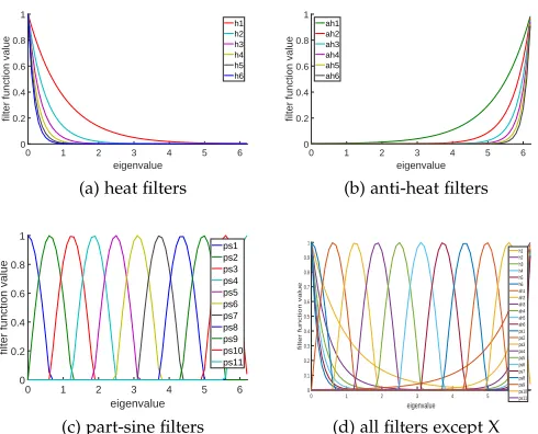
2.2 The proposed filter function sets

The heat filter set members for1≤t≤6are shown in Fig. 1(a). As it was mentioned before, their equation is:

Ht(λl) =e−tλl. (14)

(6)

0 1 2 3 4 5 6 eigenvalue

0 0.2 0.4 0.6 0.8 1

filter function value

h1 h2 h3 h4 h5 h6

(a) heat filters

0 1 2 3 4 5 6

eigenvalue 0

0.2 0.4 0.6 0.8 1

ah1 ah2 ah3 ah4 ah5 ah6

(b) anti-heat filters

0 0.2 0.4 0.6 0.8 1

ps1 ps2 ps3 ps4 ps5 ps6 ps7 ps8 ps9 ps10 ps11

(c) part-sine filters

0 0.1 0.2 0.3 0.4 0.5 0.6 0.7 0.8 0.9 1

h1 h2 h3 h4 h5 h6 ah1 ah2 ah3 ah4 ah5 ah6 ps1 ps2 ps3 ps4 ps5 ps6 ps7 ps8 ps9 ps10 ps11

[image:6.612.52.297.53.251.2]

(d) all filters except X

Fig. 1: The proposed filter function sets.

the application in hand. Here utilizing three other filter sets are proposed. The anti-heat filter set is the second used filter set, shown in Fig 1(b). These filters are computed with the following equation:

AHt(λl) =e

−t(R−λl)_, ₍₁₅₎

where R is the end point of the eigenvalues range. It can be seen that unlike the heat filter functions, in these filters, the emphasis is on the high frequencies. Unlike the heat filter set, the anti-heat filter functions are useful where the important features reside in the small interactions, so the high frequencies can not be removed. The low frequencies can be disregarded, because they possess redundant or unrelated features. The third filter set, shown in Fig. 1(c) is the part-sine filter set whose every member emphasize on a special portion of the spectrum and is calculated as follows:

P Sr,ρ(λl) =

(

sin₂π_ρ(λl−ρ(r−2)) ifρ(r−2)≤λl≤ρr

0 otherwise,

(16)

whereρis the number of sub-ranges the part-sine functions defined on and r is their sequence number. For the situ-ations that the most effective frequencies are unknown or the important information spread over the entire frequency domain, the part-sine filters are good candidates. Dividing the spectrum into different sub-ranges, separates the effects of the features of different scales. Considering the entire spectrum equips us with all the features, including effective, non-effective and noisy features. The undesired features can be removed in subsequent steps. Fig 1d displays the mentioned filters together for comparison. The last filter is X(λl) = λl. This filter is appended to the filter set for

generalizing the proposed method, as it will be shown in Section 2.4.

2.3 Pseudo-Fourier operators

FFE has the potential to be a general-purpose embedding method, because it makes use of both eigenvalues and

eigenvectors simultaneously. The effect of the eigenvalues can be adjusted in FFE by changing the filter function. Another flexibility which is needed for generalizing FFE is the feasibility of defining different combinations of eigen-vector elements. This feasibility is not provided by FFE, because it represents a linear transform of the original representation. Despite being invariant, the graph Fourier transform does not always provide so much information about the graph structure. For a constant graph signal, the Fourier transform is given byGˆ(λl) =PN_x=1φl(x)which is

equal to S1(φl)of symmetric polynomials (eq. 2). Because

of these two reasons, providing some new operators rather than Fourier transform using some different combination strategies on the elements of eigenvectors can be helpful. We call these operators as pseudo-Fourier operators (PFOs). A PFO should preserve these conditions:

1) It should possess the notion of frequency like in the Fourier transform, i.e. it should preserve the property that by moving towards the greater eigenvalues, the number of changes in the values of the eigenvector elements decreases or increases monotonically.

2) It should be able to formulate the methods which use just the eigenvalues as the special cases. For instance, the Laplacian spectrum is a relatively strong method which FFE cannot formulate.

3) It should promote the capability of pattern recognition of graphs relative to the mere use of Fourier transform in FFE. Additionally, it should formulate FFE as the special case.

The PFOs are motivated by a number of factors. Firstly, PFOs are directly related to the symmetric polynomials [14], introduced as a successful graph representation, but more convenient numerically. Secondly, we adopt the nonlinear combination of the eigenvector elements, to make our in-variant more general and informative. Finally, as pointed out for each PFO separately in the following, the proposed PFOs convey useful information about the graph structure and enrich our invariant.

Definition 2. _{Power PFO:} _{The power PFO of graph} _G _is a N ×Ω matrix named G, whose column˙ ω ∈ W = {ω1, ω2, . . . , ωΩ} is the power PFO of order ω of G and

computed as follows:

˙

Gω_{= [}PN

u=1φ1(u)ω,PNu=1φ2(u)ω, . . . ,PNu=1φN(u)ω]T.

(17)

The power PFO of order 0 is the number of graph vertices and is constant over the eigen-modes. Therefore, as it will be shown in Section 2.4, utilizing power PFO of order 0 in proposed GeFFE method, removes the effect of the eigenvector elements, so it makes possible for GeFFE to generate the effect of eigenvalue-dependent feature vectors such as the Laplacian spectrum. The power PFO of order1is the Fourier transform and it conveys the notion of frequency. The increasing powers emphasize higher-value components of the eigenvector like a kind of soft-max function. In terms of the graph structure, this emphasizes graphs where a single node has a strong response at a particular frequency, as PN

u=1φ1(u)ω will be large in this case. The transform

(7)

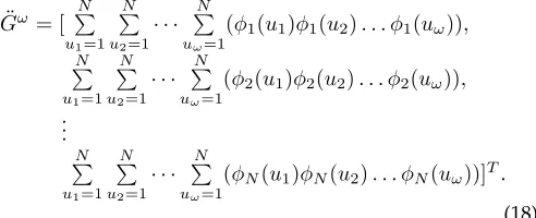
Definition 3. _{Correlated PFO:}_{The correlated PFO of graph} Gis aN ×Ωmatrix named G, whose column¨ ω ∈ W = {ω1, ω2, . . . , ωΩ}is the correlated PFO of orderωand

com-puted as follows:

¨

Gω_{= [} PN

u1=1 N

P

u2=1

· · · PN

uω=1

(φ1(u1)φ1(u2). . . φ1(uω)),

N

P

u1=1 N

P

u2=1

· · · PN

uω=1

(φ2(u1)φ2(u2). . . φ2(uω)),

.. .

N

P

u1=1 N

P

u2=1

· · · PN

uω=1

(φN(u1)φN(u2). . . φN(uω))]T.

(18)

The correlated PFO of the orders0and1are equivalent to the power PFO of the same orders. The order 2 is the first order which the information of the correlation between different entities of the eigenvector is appeared on. This PFO measures the statistical correlation between the eigenvector elements at different orders. This therefore gives a large value when the frequency response of a group of nodes is the same (i.e. they have the same relationship to the rest of the graph).

2.4 Generalized Frequency Filtering Embedding

The generalized frequency filtering embedding is defined as follows:

Definition 4. _{Generalized Frequency Filtering Embedding} (GeFFE): Let F = {F1, F2, . . . , Fr} be the filter bank and

W = {ω1, ω2, . . . , ωΩ} be the order set of the PFO. The

generalized frequency filtering embeddingγF,W is defined as:

γF,W :G →RΩ×m×r

γF,W(G) = [f1ω1(G)T,f1ω2(G)T, . . . ,f1ωΩ(G)T,

fω1

2 (G)T,f2ω2(G)T, . . . ,f2ωΩ(G)T,

.. . fω1

r (G)T,frω2(G)T, . . . ,frωΩ(G)T,],

(19)

whereG is the graph domain,mis the number of selected eigen-modes, andfω

k(G) = [Fk(λj) ˇGω(λj), j= 1, . . . , m]is

the response of orderωof graphGto the filterFk. whereGˇ

can be one ofG˙ andG, for instance.¨

In the above definition,F and W can be selected stati-cally or trained for each application. The second approach is more effective, because as it is shown in Sections 3.3 and 3.4, the best combinations of filters and PFOs vary for varying graph structures. The training process is described in Section 3.5.

By definition 4, we propose GeFFE as a general framework, which can formulate some previously-introduced invariants as the special cases, by choosing the appropriate filter function and the appropriate Fourier transform of different orders. The definitions of PFO as well as two sets F and

W for these invariants are tabulated in Table 1. As it is clarified, GeFFE can formulate both the spectrum-based invariants like Laplacian spectrum by removing the impact of the Fourier transform and the eigenvector-based invari-ants like symmetric polynomials by removing the impact

of eigenvalues. GeFFE can generate more complicated in-variants like eigen-modes and the heat content power series coefficients by getting both eigenvalues and eigenvectors involved in GeFFE vector computation. In the last case, the mth element of the embedded vectorqis:

qm=PNk=1

(PN

u=1φk(u))2 ( −λk)m

m!

. (20)

[image:7.612.53.299.97.197.2]

The embedded vector of GeFFE is more informative, because it possesses the components themselves not their summation. For full equivalence, the applied classifier should be able to simulate the impact of summation for the vector components.

TABLE 1: The Previously Defined Invariants as the Special Case of GeFFE.

InvariantF W Gˇω

Lspec {λk|k= 1,2, . . . , N} {0} G˙ω

Ftran {1|k= 1,2, . . . , N} {1} G˙ω

Poly {1|k= 1,2, . . . , N} {1,2, . . . ,|V|}G¨ω

Emod {λk|k= 1,2, . . . , N} {1} G˙ω

HIP n(−λk)1

1! , (−λk)2

2! , . . . , (−λk)m

m! |k= 1,2, . . . , N o

{2}

(PN

u=1φk(u))ω|

k= 1,2, . . . , NT

Lspec, Ftran, Poly, Emod and HIP stand for Laplacian-spectra, Fourier trans-form, Symmetric polynomials [14], Eigen-mode [6] and Heat content power series coefficients [45], respectively.

3 E

XPERIMENTAL RESULTS

In this section, some experimental results are reported to show the effect of GeFFE in differentiating and classification of different graphs with different properties. All the classi-fication accuracies are estimated using 5NN classifier and 5 fold cross validation and the average of 10 runs are reported. A set of diverse datasets collected from different related papers are used in the experiments of this paper. The graphs of mutag dataset [46] represent the chemical compounds which are classified to be mutagen or not. In PTC dataset [47] , the objective is to detect the carcinogenicity of the chemical compounds from their graphs. The graphs of Enzymes dataset [48] represent the tertiary structure of proteins in two types of enzymes. PPI [49] is the dataset of the protein-protein interaction networks in two types of bacteria. CATH2 [48] consists of the graphs of the proteins and the objective is to detect the homogeneity class. Protein dataset [50] is composed of the protein structure of six types of the enzymes. Shock dataset [51] is constructed from the skeletal structures of 2D objects. Llow, Lmed and Lhigh datasets [50] consist of the graphs of hand-writing letters with low, medium and high distortions, respectively. The objective is to detect the class (i.e. a, b, ...,z) of the input letter. COIL15 [50] and ODBK50 [52] are two object detection datasets composed of the object structural graphs whose vertices are extracted through corner detection and edges are inserted through triangulation. The properties of these datasets are tabulated in Table 2.

(8)

[image:8.612.50.296.59.218.2]

TABLE 2: The Real Graph Datasets.

Dataset #Vertices

(min, max, ave)

#Edges (min, max, ave)

#Graphs #Classes

mutag (14, 40, 26.03) (26, 84, 53.78) 188 2

PTC (2, 109, 25.56) (2, 216, 51.92) 344 2

Enzymes (2, 126, 32.63) (1, 149, 62.14) 600 2

PPI (3, 232, 109.60) (4, 3006, 864.37) 86 2

CATH2 (143, 568, 307.99) (556, 2220, 1254.8) 190 2

Protein (2, 126, 32.63) (1, 149, 62.14) 600 6

Shock (4, 33, 13.17) (6, 64, 24.33) 150 10

Llow (1, 8, 4.68) (0, 6, 3.13) 2250 15

Lmed (1, 9, 4.67) (0, 7, 3.21) 2250 15

Lhigh (1, 9, 4.67) (0, 9, 4.5) 2250 15

COIL15 (18, 77, 42.73) (45, 222, 116.49) 585 15

ODBK50 (41, 200, 123.23) (106, 589, 352.81) 600 50

(Lspec), the symmetric polynomials signature (Poly) [14], the number of backtrackless walks of different lengths (BTW) [17], Ihara zeta functions (IZF) [16], heat kernel trace (HIT) and power series expansion coefficients of heat content (HIP) [45], the number of random walks of different lengths (RW) [12], the sorted elements of wave kernel (WK) [53], the histogram and sorted values of node HKSs (KShist and HKSsort) [44].

3.1 Following the edit distance

In an appropriate embedding method, the trend of chan-ging in the feature distance should obey from the trend of changing in edit distance. It means that two graphs with small edit distance should have a small feature distance and vice versa. This behavior is studied in this experiment. For this purpose, four random graphs are produced through four different methods as the seed graphs. The first one is a Delaunay triangulation graph with 100 nodes whose(x, y)

[image:8.612.313.560.439.620.2]

coordinates are real numbers picked from [1,100] randomly. The second seed graph is an erd˝os-R´enyi model with 100 nodes and 130 edges. The third seed graph is a geometric graph with 100 nodes whose 3-dimension coordinates are picked randomly from [0,1] and two nodes are connected if they are in 0.5 radius neighborhood of each other. The last random graph is a small world graph with average degree 6 and random rewiring probability 0.2. The seed graphs are shown in the column a of the Fig. 2. In separate tests, 30 variations of every seed graph are made by random consecutive edge deletions. This process is repeated 1000 times and yields the set of 1000 graphs for every edit distance 1 to 30 from the seed graph. The column b of Fig. 2 shows the mean FFE feature distance against the edit distance for every corresponding seed graph. The filter set isF = {X} ∪ {P Sr,11|1 ≤ r ≤ 11} and the 12 filter

responses are inserted in a long vector. As it is observed, FFE cannot differentiate between edited graphs. The reason is that the positive and negative eigenvector elements cancel each other and produce the small values as the elements of Fourier transform for all graphs. The columns c and d of the Fig. 2 correspond to the long vectors of GeFFE using the mentioned filter set and the orders W = {0,1,4} of

˙

GandG, respectively. The resulting vectors have the mean-¨ ingful feature distances with each other, however the feature

distances of GeFFE byG˙ exhibit less standard deviation in average and its change is more monotonic.

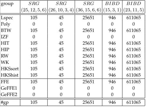
3.2 Cospectrality

The purpose of this experiment is to study the power of the proposed embedding methods to differentiate cospectral graphs. For this experiment, three groups of the strongly regular graphs (SRGs) and 2 groups of Balanced Incomplete Block Designs (BIBDs) are used. SRG(v, k, λ, µ) is a k-regularv-node graph which every pair of its adjacent nodes hasλcommon neighbors and every pair of its non-adjacent nodes hasµcommon neighbors.BIBD(v, k, λ)is av-node graph consisting of k-node blocks such that every pair of the graph nodes is placed in λ blocks. The graphs of every group has the identical parameters and the identical Laplacian spectrum, however they are not isomorphic. FFE by the identity filter (FFE), GeFFE by the identity filter and

˙

Gof order 4 (GeFFE1), and GeFFE by the identity filter and

¨

Gof order 4 (GeFFE2) are compared with each other and with previous methods in cospectrality reduction. The point should be noted is that since just one filter and one Fourier order is selected, the embedded vector length is N for all three proposed methods. The results are tabulated in Table 3. It can be seen that FFE can not differentiate the tested cospectral graphs, while both GeFFE1 and GeFFE2 are able to obtain the best possible result in this experiment. The Poly method could obtain this result, but the length of its feature vector is N2_{. IZF method is another method which could}

obtain the similar result, but inO(N6)time in comparison withO(N3₎_{of GeFFE1 and}_O₍_N5₎_{of GeFFE2.}

TABLE 3: The Amount of Cospectrality in Proposed Meth-ods.

group SRG SRG SRG BIBD BIBD

(25,12,5,6) (26,10,3,4) (36,15,6,6) (15,3,1) (23,11,5)

Lspec 105 45 25651 946 611065

Poly 0 0 0 0 0

BTW 105 45 25651 946 611065

IZF 0 0 0 0 0

HIP 105 45 25651 946 611065

RW 105 45 25651 946 611065

WK 105 45 25651 946 611065

HKSsort 105 45 25651 946 611065

HKShist 105 45 25651 946 611065

FFE 105 45 25651 946 611065

GeFFE1 0 0 0 0 0

GeFFE2 0 0 0 0 0

#gp 105 45 25651 946 611065

The tabulated numbers are the number of cospectral graph pairs. #gp stands for the total number of graph pairs in the group.

3.3 The comparison between different filters

(9)

0 5 10 15 20 25 30 Edit distance -0.5

-0.4 -0.3 -0.2 -0.1 0 0.1 0.2 0.3 0.4 0.5

Feature distance

Feature distance of FFE vs Edit distance

0 5 10 15 20 25 30 Edit distance 0

2 4 6 8 10 12

Feature distance

Feature distance of GeFFE1 vs Edit distance

0 5 10 15 20 25 30 Edit distance -10

-5 0 5 10 15 20 25 30

Feature distance

0 5 10 15 20 25 30 Edit distance 7

8 9 10 11 12 13 14 15 16 17

Feature distance

0 5 10 15 20 25 30 Edit distance 8

10 12 14 16 18 20 22

Feature distance

0 5 10 15 20 25 30 Edit distance 150

200 250 300 350 400 450 500 550 600

Feature distance

0 5 10 15 20 25 30 Edit distance 4

4.5 5 5.5 6 6.5

Feature distance

10-13 Feature distance of FFE vs Edit distance

0 5 10 15 20 25 30 Edit distance 0

5 10 15 20 25 30 35 40

Feature distance

0 5 10 15 20 25 30 Edit distance 0

2 4 6 8 10 12 14

Feature distance

0 5 10 15 20 25 30 Edit distance -1

-0.5 0 0.5 1 1.5

Feature distance

0 5 10 15 20 25 30 Edit distance 0

2 4 6 8 10 12

Feature distance

0 5 10 15 20 25 30 Edit distance -30

-20 -10 0 10 20 30 40 50 60

Feature distance

[image:9.612.61.538.45.351.2]

a b c d

Fig. 2: The feature distances of different proposed methods in comparison with the edit distance. Column a: Seed graphs. Column b: FFE method. Column c: GeFFE by power PFO. Column d: GeFFE by correlated PFO.

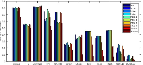
Fig. 3 plots the classification accuracies of embedded vectors of GeFFE by order 4 ofG˙ and each time by one of the filters of the set{X, H1, H3, H6, AH1, AH3, AH6, P S1,11, P S6,11,

P S11,11}for all tested datasets. It can be seen that different

filters have different effects in classification of the different datasets. We can see that the heat filters perform much better than the anti-heat on CATH2, which can be explained by the fact that the task is to find the homogeneity class which is related to large-scale structure. On the other hand, anti-heat performs better on PPI, suggesting the detailed connectivity is more important in this dataset. On the others, information is contained over the whole spectrum. The part-sine filter emphasizes narrow bands, which allows us to see where the important structure is localized to one particular scale. The notable point is that although the heat filters are known as the informative filters in different researches (but in other areas), these filters are not the best filters in all cases. Fig. 4 compares the classification accuracies of the long vectors of three different filter combinations XHAP, XAP and XP with each other. FXHAP = {X} ∪ {Ht|1 ≤

t ≤ 6} ∪ {AHt|1 ≤ t ≤ 6} ∪ {P Sr,11|1 ≤ r ≤ 11},

FXAP ={X} ∪ {AHt|1 ≤t ≤6} ∪ {P Sr,11|1 ≤r≤11},

and FXP = {X} ∪ {P Sr,11|1 ≤ r ≤ 11}. It can be seen

that the filter combination including heat filters has the lower classification accuracies in all the cases. The small scale between-node interactions, whose effect appear on high frequencies, play important role in differentiating the graphs of the applications. When heat filters attenuate the high frequencies to decrease the effect of the noise, this

beneficial information is lost as well. This behavior is shown in Fig. 5. The similar tests of Section 3.1 is performed using the long vectors constructed by orders {0,1,4} of G˙ and each time by one of the proposed filter functions. Edges are considered as representatives for small scale substructures and removing them is studied. The heat filter functions and P S1,11 filter function are worst in following edit distance.

The feature distances change very slowly and this change is not monotonic. This behavior is observed because these fil-ters alleviate the effect of changing the small scale structures in feature distance. This effect is beneficial in noise reduc-tion, where the value of these small scale substructures in differentiating the graphs is negligible; however it is not true for the applications in hand. Furthermore, although the heat kernel is known as a good solution for the problem of noise sensitivity in eigen-modes by down-weighting the high frequencies [42], but this belief is not necessarily true in all the applications. The stability of eigen-modes is dependent on the spectral gap (gap between consecutive eigenvalues) and depends on the graph structure as well as the frequency. Where noise and irrelevant local structural errors occur, this would affect the high-frequency components adversely, but this is not true of all graph data. Our experiments show this.

(10)

mutag PTC Enzymes PPI CATH2 Protein Shock llow lmed lhigh COIL15 ODBK50 0

0.1 0.2 0.3 0.4 0.5 0.6 0.7 0.8 0.9

average precision

[image:10.612.53.302.51.165.2]

X-4 H1-4 H3-4 H6-4 AH1-4 AH3-4 AH6-4 PS1-4 PS6-4 PS11-4

Fig. 3: The classification accuracies of GeFFE by some differ-ent filters and order 4 ofG.˙

comparison between different filter combinations

mutag PTC Enzymes PPI CATH2 Protein Shock llow lmed lhigh COIL15ODBK50 0

0.05 0.1 0.15 0.2 0.25 0.3 0.35 0.4 0.45 0.5 0.55 0.6 0.65 0.7 0.75 0.8 0.85 0.9

average precision

[image:10.612.57.274.219.340.2]

XHAP XAP XP

Fig. 4: The classification accuracies of some different filter combinations using three selected combination strategies.

COIL15 and ODBK50 as the similar set 2. It suggests an acceptable relation between the frequency filtering operator and graph structure and makes the hope that the GeFFE strategy is effective enough to extract the similar structures in different datasets, however the approval of this claim needs more investigation.

3.4 The comparison between different PFO orders The experiment similar to the experiment of the previous section is done for different PFO orders to show the benefits of using them. The GeFFE vectors ofP S4,11filter, each time

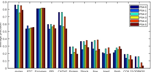
with one of the orders of the set{0,1,2,3,4,5}ofG˙are used in this experiment and the accuracies is plotted in Fig. 7 for all tested datasets. The similar effect of the previous sub-section is observable for different orders. The effectiveness of a special order differs from a dataset to another. For example, the order 0 has the highest importance in mutag, PPI and CATH2 and the lowest importance in PTC and lhigh. The similar effect can be observed in order 4 which is the most important order in Enzymes, Shock, llow, lmed and lhigh datasets, while it has the third rank in PTC, Protein, COIL15 and ODBK50. The ability of discovering similar structures can be seen more and less in this experiment, too. This results and the results of the previous sub-section suggest that different combinations of the filters and the Fourier orders include useful information and the appro-priate combination of them should be applied based on the application in hand. Different datasets have different properties, and machine learning can use these features to learn the most appropriate representation.

3.5 GeFFE vs other embedding methods

The main purpose of embedding methods is to map the similar graphs into close vectors and the dissimilar graphs into far ones. The experiment reported in Section 3.1 showed that GeFFE vectors exhibited this property in a synthetic graph set. The purpose of this experiment is to evaluate GeFFE for having the mentioned property in real graphs. Classification using the simple classifier 5NN can help us to estimate the amount of this property.

GeFFE by the filter set F = {X} ∪ {Ht|1 ≤ t ≤ 6} ∪

{AHt|1 ≤ t ≤ 6} ∪ {P Sr,11|1 ≤ r ≤ 11} and the

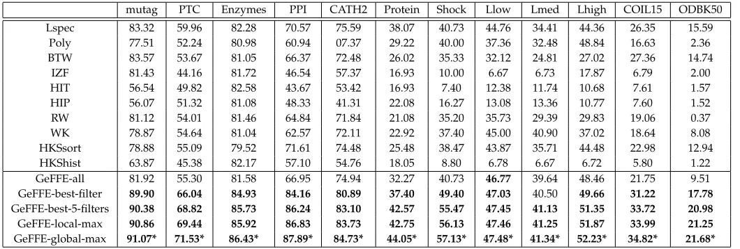
order set W = {0,1,4} of G˙ is compared with the other embedding methods in Table 5. In the first version of the method, GeFFE-all, the long vector of all filter responses is considered as the feature vector. GeFFE-all obtained the average rank 2.58 among 11 tested methods, which makes it comparable with the other methods. However,GeFFE-allcan not reach the best accuracy in all tested datasets. The reason is that as it is shown in Section 3.3 and Section 3.4, different filters and different orders have different importance in different datasets, but inGeFFE-all, all of the filter responses are inserted into the feature vector and participate in the clustering process with the same importance, regardless of the properties of the underlying dataset. Consequently, for taking full advantage of the information revealed by the filter responses, it is necessary to learn the importance degree of each filter response and use this degree in the clustering process.

We followed this aim by applying forward selection on filter responses. The graph response to the specific filter and the specific order of PFO is considered as a feature group, yieldingr×Ωfeature groups. The forward selection starts with an empty feature set and at each step, the feature group which better enhances the classification accuracy in training data is added to the selected feature groups. 10 first selected feature groups for the tested datasets are tabulated in Table 4. According to these results, 4 versions of GeFFE are applied to the datasets and the results are reported in Table 5. The feature vectors ofGeFFE-best-filterand GeFFE-best-5-filters are composed of the first and 5 first selected feature groups in forward selection process, respectively. In GeFFE-local-max, the selected feature groups are used until the step where its 10 future steps could not enhance the accuracy. InGeFFE-global-max, the feature groups are used until the step where the max accuracy in training data is obtained. The average number of filter responses in GeFFE-local-maxandGeFFE-global-maxover tested datasets are 7.08 and 17.08, respectively. As it can be seen,GeFFE-global-maxis the best performing method. However the other 3 versions of GeFFE outperforms the previous methods in all the tested datasets (except a case of GeFFE-best-filter where the difference is negligible). The first point that can be perceived from the results is that the selected filters and PFOs are efficient enough for our purpose and the second point is that our strategy in selecting suitable filter responses for the datasets could adopt GeFFE to the structural properties of different datasets.

(11)

0 5 10 15 20 25 30 Edit distance -0.2 -0.1 0 0.1 0.2 0.3 0.4 0.5 0.6 0.7 0.8 Feature distance

Feature distance of H1 vs Edit distance

0 5 10 15 20 25 30

Edit distance -0.3 -0.2 -0.1 0 0.1 0.2 0.3 0.4 0.5 0.6 0.7 Feature distance

0 5 10 15 20 25 30

Edit distance -0.3 -0.2 -0.1 0 0.1 0.2 0.3 0.4 0.5 0.6 Feature distance

0 5 10 15 20 25 30

Edit distance -0.4 -0.3 -0.2 -0.1 0 0.1 0.2 0.3 0.4 0.5 0.6 Feature distance

0 5 10 15 20 25 30

Edit distance -0.2 0 0.2 0.4 0.6 0.8 1 Feature distance

Feature distance of AH1 vs Edit distance

0 5 10 15 20 25 30

Edit distance -0.2 0 0.2 0.4 0.6 0.8 1 1.2 Feature distance

0 5 10 15 20 25 30

H1 H2 H3 H4 H5 H6 AH1 AH2 AH3 AH4 AH5 AH6

0 5 10 15 20 25 30

Edit distance -0.1 0 0.1 0.2 0.3 0.4 0.5 0.6 0.7 0.8 0.9 Feature distance

Feature distance of PS1 vs Edit distance

0 5 10 15 20 25 30

Edit distance 0 0.2 0.4 0.6 0.8 1 1.2 1.4 Feature distance

0 5 10 15 20 25 30

Edit distance 0 0.5 1 1.5 2 2.5 Feature distance

0 5 10 15 20 25 30

Edit distance 0 0.5 1 1.5 2 2.5 3 Feature distance

0 5 10 15 20 25 30

Edit distance 0 0.5 1 1.5 2 2.5 3 3.5 Feature distance

0 5 10 15 20 25 30

Edit distance 0 0.5 1 1.5 2 2.5 3 Feature distance

0 5 10 15 20 25 30

Edit distance 0 0.5 1 1.5 2 2.5 Feature distance

0 5 10 15 20 25 30

Edit distance -0.2 0 0.2 0.4 0.6 0.8 1 1.2 1.4 1.6 Feature distance

0 5 10 15 20 25 30

Edit distance 0 1 2 3 4 5 6 7 8 9 Feature distance

Feature distance of X vs Edit distance

[image:11.612.56.571.42.136.2]

P S1,11 P S2,11 P S3,11 P S4,11 P S5,11 P S6,11 P S7,11 P S8,11 P S9,11 P S10,11 P S11,11 X

[image:11.612.62.549.182.308.2]

Fig. 5: The test of following edit distance for proposed filter functions.

TABLE 4: The 10 First Selected Filter Responses Using Forward Selection on the GeFFE Filter Responses.

mutag PTC Enzymes PPI CATH2 Protein Shock Llow Lmed Lhigh COIL15 ODBK50

1 AH5-0 X-1 P S11-0 AH4-0 AH3-0 AH2-0 AH6-0 P S11-0 P S11-0 P S11-0 AH4-0 AH1-0

2 AH6-0 AH2-1 AH6-0 AH6-0 AH2-0 AH3-0 AH5-0 AH6-1 AH4-1 AH6-1 AH3-0 AH2-0

3 X-1 AH3-1 AH4-0 AH3-0 AH5-0 X-0 AH3-0 AH2-1 AH5-1 AH5-1 AH5-0 AH3-0

4 AH4-0 AH6-1 AH3-0 AH5-0 AH4-0 AH4-0 AH4-0 AH3-1 AH3-1 AH4-1 X-1 AH4-0

5 AH3-0 AH4-1 AH5-0 AH2-0 AH1-0 AH5-0 AH2-0 AH4-1 AH6-1 P S11-1 AH6-0 AH5-0

6 AH2-1 AH5-1 AH2-0 P S10-0 AH6-0 AH1-0 AH1-0 AH5-1 AH2-1 P S10-1 AH2-0 AH6-0

7 AH3-1 AH1-1 AH4-1 P S9-0 X-1 AH6-0 P S11-0 AH1-1 P S11-1 AH3-1 P S11-0 X-1

8 AH1-1 AH6-0 X-1 P S7-0 P S11-0 P S11-0 AH3-1 P S6-1 AH1-1 P S11-4 AH1-1 AH1-1

9 AH2-0 P S2-1 AH2-1 P S8-0 AH1-1 X-1 AH2-1 H2-0 P S10-1 P S10-0 AH2-1 P S11-0

10 AH4-1 P S4-1 AH3-1 P S11-0 AH2-1 AH1-1 AH4-1 H1-0 P S6-1 AH2-1 AH3-1 AH2-1

P Si,11is briefly indicated byP Si.

Fig. 6: The similar reactions of different filters on the struc-turally similar datasets. The similar set 1 is {Llow, Lmed and Lhigh}and the similar set 2 is{COIL15 and ODBK50}.

mutag PTC Enzymes PPI CATH2 Protein Shock llow lmed lhigh COIL15 ODBK50 0 0.1 0.2 0.3 0.4 0.5 0.6 0.7 0.8 0.9 average precision PS4-0 PS4-1 PS4-2 PS4-3 PS4-4 PS4-5

Fig. 7: The classification accuracies of GeFFE byP S4,11filter

and different orders ofG.˙

GeFFE method using power PFOs is ofO(N)and its time complexity is of O(N3) just like the majority of the other spectral methods. Of course, its training time depends on the used feature selection strategy.

4 C

ONCLUSION

In this article, a novel embedding method named GeFFE is proposed using the graph signal processing operators: fre-quency filtering and Fourier transform. Frefre-quency filtering amplifies or attenuates the contribution of different eigen-values and the proposed pseudo-Fourier operators expands graph Fourier transform to make diverse invariant combi-nations of eigenvector elements. The conclusion remarks of this article can be listed as follows:

1) GeFFE benefits from the information of both eigen-values and eigenvectors, hence it has the ability of discovering:

(a) Structural similarities. GeFFE (especially by power PFOs) can simulate the edit distance in random vari-ations of a seed graph.

(b) Structural differences: GeFFE by both power and correlated PFOs can differentiate some groups of Laplacian cospectral graphs from each other entirely. 2) GeFFE has the ability to concentrate on a special por-tion of the spectrum and explore its latent structural information. In this regard:

(a) Some filter functions were proposed. It was experi-mentally shown that some filter sets excluding the heat filters results in better classification accuracies. This observation opens the possibility of discovering more powerful filter functions.

(b) Different filter functions are different in graph classi-fication. So training their importance in the applica-tion in hand is beneficial.

[image:11.612.49.301.336.447.2] [image:11.612.52.302.516.634.2]

(12)

[image:12.612.46.576.59.238.2]

TABLE 5: The Classification Accuracies of Some Versions of GeFFE in Comparison With the Existing Embedding Methods.

mutag PTC Enzymes PPI CATH2 Protein Shock Llow Lmed Lhigh COIL15 ODBK50

Lspec 83.32 59.96 82.28 70.57 75.59 38.07 40.73 44.76 34.41 44.36 26.35 15.59

Poly 77.51 52.24 80.98 60.94 07.37 29.22 40.00 37.36 32.48 48.84 16.63 2.36

BTW 83.57 53.67 81.05 66.37 72.48 26.02 35.33 32.12 24.81 27.02 27.36 14.74

IZF 81.43 44.16 81.72 46.54 57.37 16.93 10.00 6.67 6.73 17.87 6.79 2.00

HIT 56.54 49.82 82.58 43.67 53.42 16.93 7.40 12.38 11.74 10.68 7.61 1.57

HIP 56.07 51.32 81.08 48.33 41.31 22.08 16.27 13.08 13.36 10.77 7.60 1.52

RW 81.12 54.01 81.46 64.84 71.84 21.08 35.20 35.73 29.39 29.83 19.06 0.37

WK 78.87 54.64 81.04 62.57 72.11 22.92 37.40 45.00 40.90 37.02 18.64 8.08

HKSsort 78.88 55.09 79.52 71.61 74.48 25.48 38.47 43.87 35.71 44.48 22.98 12.94

HKShist 63.87 45.38 82.17 57.10 54.76 18.05 8.80 6.78 6.67 6.72 5.80 1.22

GeFFE-all 81.92 55.30 81.58 66.95 74.94 32.27 40.73 46.77 _39.64 _48.46 _21.75 _9.51

GeFFE-best-filter 89.90 66.04 84.93 84.16 80.89 37.40 49.40 47.03 40.50 49.66 31.22 17.78

GeFFE-best-5-filters 90.38 68.82 85.73 86.24 83.10 42.57 55.47 47.45 41.13 51.35 33.72 20.98

GeFFE-local-max 90.86 69.44 85.92 86.83 83.73 42.75 56.13 47.46 41.25 51.87 33.99 21.25

GeFFE-global-max 91.07* 71.53* 86.43* 87.89* 84.73* 44.05* 57.13* 47.48* 41.34* 52.23* 34.82* 21.68*

The best accuracies for each dataset is determined by the * symbol.

The accuracies of GeFFE versions which are better than all the accuracies of the other previous methods are indicated with bold face.

different datasets.

3) Training the best performing filter responses through forward selection is a good strategy for adopting GeFFE to the structural properties of different datasets. Through this strategy, GeFFE even using just the best filter response has the superior performances against existing embedding methods in classification the tested datasets.

4) GeFFE can play the role of the general framework to formulate some graph invariants which make use of eigenvalues, eigenvectors or both of them.

5) GeFFE has the potential to be more efficient by defining other filters in order to explore the spectrum more precisely and other PFOs in order to combine the eigen-vector elements in different ways.

For further assessment on this new trend, we plan to explore the new filter functions as well as the new methods for com-posing PFOs. Some specially-designed synthetic datasets can be helpful for designing a useful filter-bank which each of its members is appropriate for discovering a special graph substructure. A similar investigation should be done for dis-covering the detailed relation between different PFOs and PFO orders with graph structures. A method is needed to discover more informative portions of the spectrum for each dataset and analyze this portion more precisely. Spectral invariants usually consider only unlabeled or sometimes labeled graphs, but not attributes. Using graph signal gives GeFFE the potential of handling attributed graphs, however this potential ability should be investigated in detail.

R

EFERENCES

[1] C. M. Bishop,Pattern recognition and machine learning. Springer,

2006.

[2] K. Fukunaga, Introduction to statistical pattern recognition.

Aca-demic press, 2013.

[3] M. Alvarez Vega, “Graph kernels and applications in

bioinformat-ics,” Ph.D. dissertation, Utah State University, 2011.

[4] H. Bunke and K. Riesen, “Recent advances in graph-based

pat-tern recognition with applications in document analysis,”Pattern

Recognition, vol. 44, no. 5, pp. 1057–1067, 2011.

[5] H.-P. Kriegel, P. Kr ¨oger, M. Renz, and T. Schmidt, “Hierarchical

graph embedding for efficient query processing in very large

traf-fic networks,” inInternational Conference on Scientific and Statistical

Database Management. Springer, 2008, pp. 150–167.

[6] B. Luo, R. C. Wilson, and E. R. Hancock, “Spectral embedding of

graphs,”Pattern recognition, vol. 36, no. 10, pp. 2213–2230, 2003.

[7] S. G ¨unter and H. Bunke, “Self-organizing map for clustering in

the graph domain,”Pattern Recognition Letters, vol. 23, no. 4, pp.

405–417, 2002.

[8] H. Bunke and K. Riesen, “Towards the unification of structural and

statistical pattern recognition,”Pattern Recognition Letters, vol. 33,

no. 7, pp. 811–825, 2012.

[9] J. Gibert, E. Valveny, and H. Bunke, “Graph embedding in vector

spaces by node attribute statistics,” Pattern Recognition, vol. 45,

no. 9, pp. 3072–3083, 2012.

[10] D. Haussler, “Convolution kernels on discrete structures,” Cite-seer, Tech. Rep., 1999.

[11] R. I. Kondor and J. Lafferty, “Diffusion kernels on graphs and other

discrete input spaces,” inICML, vol. 2, 2002, pp. 315–322.

[12] T. G¨artner, P. Flach, and S. Wrobel, “On graph kernels: Hardness

results and efficient alternatives,” in Learning Theory and Kernel

Machines. Springer, 2003, pp. 129–143.

[13] H. Bunke, S. G ¨unter, and X. Jiang, “Towards bridging the gap between statistical and structural pattern recognition: Two new

concepts in graph matching,” in International Conference on

Ad-vances in Pattern Recognition. Springer, 2001, pp. 1–11.

[14] R. C. Wilson, E. R. Hancock, and B. Luo, “Pattern vectors from

algebraic graph theory,”IEEE Transactions on Pattern Analysis and

Machine Intelligence, vol. 27, no. 7, pp. 1112–1124, 2005.

[15] P. Ren, R. C. Wilson, and E. R. Hancock, “Spectral embedding

of feature hypergraphs,” inJoint IAPR International Workshops on

Statistical Techniques in Pattern Recognition (SPR) and Structural and Syntactic Pattern Recognition (SSPR). Springer, 2008, pp. 308–317.

[16] ——, “Graph characterization via ihara coefficients,”IEEE

Trans-actions on Neural Networks, vol. 22, no. 2, pp. 233–245, 2011. [17] F. Aziz, R. C. Wilson, and E. R. Hancock, “Backtrackless walks on

a graph,”IEEE transactions on neural networks and learning systems,

vol. 24, no. 6, pp. 977–989, 2013.

[18] B. Xiao, “Heat kernel analysis on graphs,” Ph.D. dissertation, The University of York, 2007. 2, 2007.

[19] H. Bahonar, A. Mirzaei, and R. C. Wilson, “Diffusion wavelet embedding: A multi-resolution approach for graph embedding in

vector space,”Pattern Recognition, vol. 74, pp. 518–530, 2018.

[20] B. Bonev, F. Escolano, D. Giorgi, and S. Biasotti, “Information-theoretic selection of high-dimensional spectral features for

struc-tural recognition,”Computer Vision and Image Understanding, vol.

117, no. 3, pp. 214–228, 2013.

[21] R. N. Bracewell and R. N. Bracewell,The Fourier transform and its

applications. McGraw-Hill New York, 1986, vol. 31999.

[22] J. S. Lim, “Two-dimensional signal and image processing,”

(13)

[23] J. Brault and O. White, “The analysis and restoration of

astronomi-cal data via the fast fourier transform,”Astronomy and Astrophysics,

vol. 13, p. 169, 1971.

[24] J. R. Ferraro and L. J. Basile,Fourier Transform Infrared Spectra:

Applications to Chemical Systems. Academic press, 2012.

[25] D. I. Shuman, S. K. Narang, P. Frossard, A. Ortega, and P. Van-dergheynst, “The emerging field of signal processing on graphs: Extending high-dimensional data analysis to networks and other

irregular domains,”IEEE Signal Processing Magazine, vol. 30, no. 3,

pp. 83–98, 2013.

[26] F. Zhang and E. R. Hancock, “Graph spectral image smoothing

using the heat kernel,”Pattern Recognition, vol. 41, no. 11, pp. 3328–

3342, 2008.

[27] D. K. Hammond, P. Vandergheynst, and R. Gribonval, “Wavelets

on graphs via spectral graph theory,”Applied and Computational

Harmonic Analysis, vol. 30, no. 2, pp. 129–150, 2011.

[28] W.-S. Kim, S. K. Narang, and A. Ortega, “Graph based transforms

for depth video coding,” in2012 IEEE International Conference on

Acoustics, Speech and Signal Processing (ICASSP). IEEE, 2012, pp. 813–816.

[29] M. Crovella and E. Kolaczyk, “Graph wavelets for spatial traffic

analysis,” inINFOCOM 2003. Twenty-Second Annual Joint

Confer-ence of the IEEE Computer and Communications. IEEE Societies, vol. 3. IEEE, 2003, pp. 1848–1857.

[30] N. Sidere, P. H´eroux, and J.-Y. Ramel, “A vectorial representation

for the indexation of structural informations,”Structural, Syntactic,

and Statistical Pattern Recognition, pp. 45–54, 2008.

[31] M. M. Luqman, J.-Y. Ramel, J. Llad ´os, and T. Brouard, “Fuzzy

multilevel graph embedding,”Pattern Recognition, vol. 46, no. 2,

pp. 551–565, 2013.

[32] J. Gibert, E. Valveny, and H. Bunke, “Feature selection on node

statistics based embedding of graphs,”Pattern Recognition Letters,

vol. 33, no. 15, pp. 1980–1990, 2012.

[33] E. Pekalska and R. P. Duin, “Classifiers for dissimilarity-based

pattern recognition,” inPattern Recognition, 2000. Proceedings. 15th

International Conference on, vol. 2. IEEE, 2000, pp. 12–16. [34] K. Riesen and H. Bunke, “Graph classification based on vector

space embedding,”International Journal of Pattern Recognition and

Artificial Intelligence, vol. 23, no. 06, pp. 1053–1081, 2009.

[35] E. Z. Borzeshi, M. Piccardi, K. Riesen, and H. Bunke,

“Discrimina-tive prototype selection methods for graph embedding,”Pattern

[36] A. Fischer, K. Riesen, and H. Bunke, “An experimental study of

graph classification using prototype selection,” inPattern

Recogni-tion, 2008. ICPR 2008. 19th International Conference on. IEEE, 2008, pp. 1–4.

[37] R. P. Duin and E. Pekalska, “The dissimilarity space: Bridging

structural and statistical pattern recognition,”Pattern Recognition

Letters, vol. 33, no. 7, pp. 826–832, 2012.

[38] K. Riesen and H. Bunke, “Classifier ensembles for vector space

embedding of graphs,” inInternational Workshop on Multiple

Clas-sifier Systems. Springer, 2007, pp. 220–230.

[39] ——, “Approximate graph edit distance computation by means

of bipartite graph matching,”Image and Vision computing, vol. 27,

no. 7, pp. 950–959, 2009.

[40] F. R. Chung,Spectral graph theory. American Mathematical Soc.,

1997, vol. 92.

[41] H. El-Ghawalby and E. R. Hancock, “Geometric characterizations

of graphs using heat kernel embeddings,” inIMA International

Conference on Mathematics of Surfaces. Springer, 2009, pp. 124–142. [42] J. Sun, M. Ovsjanikov, and L. Guibas, “A concise and provably

in-formative multi-scale signature based on heat diffusion,”Computer

graphics forum, vol. 28, no. 5, pp. 1383–1392, 2009.

[43] B. Xiao, E. R. Hancock, and R. C. Wilson, “Geometric character-ization and clustering of graphs using heat kernel embeddings,”

Image and Vision Computing, vol. 28, no. 6, pp. 1003–1021, 2010. [44] R. C. Wilson, “Graph signatures for evaluating network models,”

inPattern Recognition (ICPR), 2014 22nd International Conference on. IEEE, 2014, pp. 100–105.

[45] B. Xiao, E. R. Hancock, and R. C. Wilson, “Graph characteristics

from the heat kernel trace,”Pattern Recognition, vol. 42, no. 11, pp.

2589–2606, 2009.

[46] A. K. Debnath, R. L. Lopez de Compadre, G. Debnath, A. J. Shusterman, and C. Hansch, “Structure-activity relationship of mutagenic aromatic and heteroaromatic nitro compounds.

correla-tion with molecular orbital energies and hydrophobicity,”Journal

of medicinal chemistry, vol. 34, no. 2, pp. 786–797, 1991.

[47] G. Li, M. Semerci, B. Yener, and M. J. Zaki, “Effective graph

classification based on topological and label attributes,”Statistical

Analysis and Data Mining, vol. 5, no. 4, pp. 265–283, 2012. [48] L. Bai and E. R. Hancock, “Depth-based complexity traces of

graphs,”Pattern Recognition, vol. 47, no. 3, pp. 1172–1186, 2014.

[49] F. Escolano, E. R. Hancock, and M. A. Lozano, “Heat diffusion:

Thermodynamic depth complexity of networks,”Physical Review

E, vol. 85, no. 3, p. 036206, 2012.

[50] K. Riesen and H. Bunke, “Iam graph database repository for

graph based pattern recognition and machine learning,” inJoint

IAPR International Workshops on Statistical Techniques in Pattern Recognition (SPR) and Structural and Syntactic Pattern Recognition (SSPR). Springer, 2008, pp. 287–297.

[51] L. Bai, L. Rossi, A. Torsello, and E. R. Hancock, “A quantum

jensen–shannon graph kernel for unattributed graphs,” Pattern

[52] S. F. Mousavi, M. Safayani, A. Mirzaei, and H. Bahonar, “Hier-archical graph embedding in vector space by graph pyramid,”

Pattern Recognition, vol. 61, pp. 245–254, 2017.

[53] M. Aubry, U. Schlickewei, and D. Cremers, “The wave kernel signature: A quantum mechanical approach to shape analysis,” inComputer Vision Workshops (ICCV Workshops), 2011 IEEE Interna-tional Conference on. IEEE, 2011, pp. 1626–1633.

Hoda Bahonarreceived her B.Sc and M.Sc. in computer engineering from Payam noor Univer-sity and Tarbiat Modares UnvierUniver-sity, in 2005 and 2009 respectively. She is currently pursuing her Ph.D. in Computer Engineering at Isfahan Uni-versity of Technology, Isfahan, Iran. Her current research interests include Statistical and Struc-tural Pattern Recognition and Graph clustering and classification.

Abdolreza Mirzaei received the B.Sc., M.Sc. and Ph.D. degrees in 2001, 2003, and 2009, respectively, from Isfahan University, Iran Uni-versity of Science and Technology, and Amirk-abir University of Technology. He is currently an assistant professor in the electrical and com-puter engineering department at Isfahan Uni-versity of Technology, Iran. His research areas include Pattern Recognition, Machine Learning, Data Mining, and Swarm Intelligence.

Saeed Sadrireceived the B.S. and M.S. degrees in electrical engineering from the University of Tehran, Tehran, Iran, in 1977 and the Ph.D. degree from Isfahan University of Technology (IUT), Isfahan, Iran. Since 1980, he has been with the Department of Electrical and Computer Engineering, IUT. His research interests include signal and image processing, particularly image segmentation, with applications both in industry and medical science. He is a member of the DSP Laboratory, IUT, where he is engaged in computer vision, image processing, and data analysis.