A Unified Approach to Collaborative
Filtering via Linear Models and Beyond
Suvash Sedhain
A thesis submitted for the degree of
Doctor of Philosophy of
The Australian National University
Supervisor
Scott Sanner
Assistant Professor, University Of Toronto Toronto, Canada.
Co-Supervisor
Aditya Krishna Menon
Senior Researcher, DATA61
Adjunct Assistant Professor, The Australian National University Canberra ACT, Australia
Advisor
Lexing Xie
Associate Professor, The Australian National University Contributed Researcher, DATA61
Declaration
I hereby declare that this thesis is my original work which has been done in collaboration with other researchers. This document has not been submitted for any other degree or award in any other university or educational institution. The following papers are accepted for publication in peer reviewed conference proceedings listed in a reverse chronological order:
• (Chapter 4)S. Sedhain, A. Menon, S. Sanner, L. Xie, LoCo: Social Cold-Start Recommendation
via Low-Rank Regression. In Proceedings of 31st AAAI Conference on Artificial Intelligence (AAAI-16), San Francisco, USA.
• (Chapter 5)S. Sedhain, H. Bui, J. Kawale, N. Vlassis, B. Kveton, A. Menon, S. Sanner, T. Bui Practical Linear Models for Large-Scale One-Class Collaborative Filtering. In Proceedings of 25th International Joint Conference on Artificial Intelligence (IJCAI-16), NY, USA.
• (Chapter 5) S. Sedhain, A. Menon, S. Sanner, D. Braziunas, On the Effectiveness of Linear Models for One-Class Collaborative Filtering. In Proceedings of 30th AAAI Conference on Artificial Intelligence (AAAI-16), Phoenix, USA.
• (Chapter 6)S. Sedhain, A. Menon, S. Sanner, and L. Xie, AutoRec: Autoencoders Meet
Collab-orative Filtering. In Proceedings of the 24th International World Wide Web Conference (WWW-15), Florence, Italy.
• (Chapter 4)S. Sedhain, S. Sanner, D. Braziunas, L. Xie, and J. Christensen, Social
Collabo-rative Filtering for Cold-start Recommendations. In Proceedings of the ACM Conference on Recommender Systems (RecSys-14). Silicon Valley, USA.
• (Chapter 3)S. Sedhain, S. Sanner, L. Xie, R. Kidd, K.-N. Tran, and P. Christen Social Affinity Filtering: Recommendation through Fine-grained Analysis of User Interactions and Activities. In Proceedings of the ACM Conference on Online Social Networks (COSN-13). Boston, USA.
Suvash Sedhain
14 June 2017
Acknowledgments
I would like to express my sincere gratitude to everyone who made this thesis possible.
First of all, I would like to express my deepest gratitude to my supervisor, Dr. Scott Sanner, for all his guidance, patience and support throughout my doctoral study. Scott’s immense knowledge, enthusiasm, and inspiration always helped me to stay motivated. I am grateful to him for advising not only as a doctoral supervisor but also as a good friend during the hard times. In short, I couldn’t have imagined having a better supervisor for my Ph.D.
I would like to thank my co-supervisor, Dr. Aditya Krishna Menon, for helping me to grow as a researcher. His in-depth knowledge and remarkable ability to explain things in a simplest possible way made research fun for me. He has been a great mentor and a friend with whom I could discuss topics ranging from science to Game of Thrones. Further, I would like to thank my co-supervisor,Dr. Lexing Xie, for her immense support, encouragement, and helpful suggestions. I would like to express my sincere gratitude for her generosity in providing me the computational resources without which I couldn’t have done my research.
I acknowledge the financial, academic and technical support provided by the National ICT of Aus-tralia (NICTA) and the AusAus-tralian National University (ANU) for my doctoral program.
I am indebted to my colleagues at NICTA and ANU for providing a friendly environment that al-lowed me to grow as a person. Thank you for your stimulating discussions and support through the entire process. My special thanks to Trung Nguyen, Kar Wai Lim, Fazlul Hasan Siddiqui, Shamin Kinathil, Swapnil Mishra, Hadi Mohasel Afshar, Shahin Namin, Dana Pordel, Brendan Van Rooyen and Daniel McNamara. I would like to thank my friends Niroj Sapkota, Hira Babu Pradhan and Saroj Gautam for always being there for me.
I would like to thank Darius Braziunas for hosting my internship at Rakuten Kobo, and Jaya Kawale and Hung Bui for hosting my internship at Adobe Research.
I am grateful to my wife Komal Agarwal for her encouragement, unconditional love, and support throughout my PhD. I would like to thank my brother, Surendra Sedhain, and sisters, Bhagabati Sedhain, Suma Sedhain and Shova Sedhain for their love and support. I am also grateful to my niece Aatmiya Silwal and Samipya Mainali for always bringing a smile to my face.
Finally, and most importantly, I would like to thank my parents, Keshav Raj Sharma Sedhain and Chandra Kumari Sedhain. I couldn’t have done this without their guidance, encouragement, unfath-omable love and support. I dedicate this thesis to them.
Abstract
Recommending a personalised list of items to users is a core task for many online services such as Ama-zon, Netflix, and Youtube. Recommender systems are the algorithms that facilitate such personalised recommendation. Collaborative filtering (CF), the most popular class of recommendation algorithm, exploits the wisdom of the crowd by predicting users’ preferences not only from her past actions but also from the preferences of other like-minded users. In general, it is desirable to have a CF framework that is (1) applicable to wide range of recommendation scenarios, (2) learning-based, (3) amenable to convex optimisation, and (4) scalable. However, all existing CF methods, such as neighbourhood and matrix factorisation, lack one or more of these desiderata.
In this dissertation, we investigate linear models, an under-appreciated but promising area for recom-mendations that addresses all the above desiderata. We formulate a unified framework based on linear models that yields CF algorithms for four prevalent scenarios. First, we investigateSocial CF, which in-volves leveraging users’ signals from online social networks. We propose social affinity filtering (SAF), that exploits fine-grained user interactions and activities in a social network. Second, we investigate
Cold-Start CF, which refers to the scenario when we do not have any historical data about a user or an item. We formulate a large-scale linear model that leverages users social information. Third, we investigateOne-Class CF, which concerns suggesting relevant items to users from the data that consists of only positive preferences such as item purchase.Noting the superior performance of linear models, we propose LRec, a user-focused linear CF model, and extend it to large-scale datasets via dimension-ality reduction. Finally, we investigateExplicit Feedback CF, which concerns predicting user’s actual preferences such as rating, or like/dislikes. We identify CF as an auto-encoding problem and propose AUTOREC, a generalized neural network architecture for CF. We demonstrate state-of-the-art perfor-mance of the proposed models through extensive experimentation on real world datasets.
In a nutshell, this dissertation elucidates the power of linear models for various CF tasks and paves the way for further research on applying deep learning models to CF.
Contents
Declaration v
Acknowledgments ix
Abstract xi
List of Figures xvii
List of Tables xix
List of Symbols xxi
1 Introduction 1
1.1 Background: Personalised recommendation . . . 1
1.2 Motivation: What is lacking in existing CF algorithms? . . . 2
1.3 Our approach to CF: Linear models and beyond . . . 3
1.3.1 Linear models for recommendation . . . 3
1.3.2 Beyond linear models . . . 3
1.4 Key contributions of dissertation . . . 3
1.5 Outline of dissertation . . . 5
2 Overview of Recommender Systems 7 2.1 Recommendation problem: Formal definition . . . 7
2.2 Approaches to recommendation . . . 8
2.2.1 Content based filtering (CBF) . . . 8
2.2.2 Collaborative filtering (CF) . . . 8
2.3 Collaborative filtering models . . . 9
2.3.1 Neighbourhood models (KNN) . . . 9
2.3.2 Matrix factorisation models (MF) . . . 10
2.4 Collaborative filtering scenarios . . . 11
2.4.1 Explicit feedback CF . . . 11
2.4.2 One-class CF . . . 12
2.4.3 Cold-start CF . . . 15
2.4.4 Social CF . . . 16
2.5 Evaluation of recommender systems . . . 17
2.5.1 Error based metrics . . . 18
2.5.2 Ranking metrics . . . 18
2.6 Summary . . . 19
3 Linear Models for Social Recommendation 21
3.1 Problem statement . . . 21
3.2 Background . . . 21
3.3 Social affinity filtering . . . 22
3.3.1 Social signals . . . 22
3.3.2 Social affinity features from social signals . . . 25
3.3.3 Recommendation model . . . 25
3.3.4 Model analysis . . . 25
3.4 Experiment and evaluation . . . 26
3.4.1 Data description . . . 27
3.4.2 Model comparision . . . 28
3.4.3 Performance analysis . . . 29
3.4.4 Cold-Start evaluation . . . 30
3.4.5 Interaction analysis . . . 32
3.4.6 Activity analysis . . . 32
3.5 Related work and discussion . . . 35
3.6 Conclusion . . . 37
4 Linear Models for Cold-Start Recommendation 39 4.1 Problem setting . . . 39
4.2 Background . . . 39
4.2.1 Neighbourhood based cold-start CF . . . 40
4.2.2 MF based cold-start CF . . . 40
4.2.3 Limitations of existing approaches . . . 41
4.3 Linear models for cold-start recommendation . . . 41
4.3.1 Generalised neighbourhood (Gen-Neighbourhood) based cold-start model . . . . 42
4.3.2 Low linear cold-start (LoCo) model . . . 43
4.4 Relation to existing models . . . 43
4.4.1 Neighbourhood model . . . 44
4.4.2 CMF model . . . 44
4.4.3 BPR-LinMap model . . . 44
4.5 Experiment and evaluation . . . 45
4.5.1 Data description . . . 45
4.5.2 Model comparison . . . 45
4.5.3 Results and analysis . . . 46
4.6 Conclusion . . . 50
5 Linear Models for One-Class Collaborative Filtering 51 5.1 Problem setting . . . 51
5.2 LRec: Linear model for OC-CF . . . 51
5.2.1 A linear classification perspective . . . 52
5.2.2 A positive and unlabelled perspective . . . 53
5.2.3 Properties of LRec . . . 53
5.3 Extensions of LRec . . . 53
5.3.1 Incorporating side-information . . . 53
Contents xv
5.3.3 Subsampling negatives . . . 54
5.4 Relation to existing models . . . 55
5.4.1 Relation to SLIM . . . 55
5.4.2 Relation to neighbourhood methods . . . 55
5.4.3 Relation to matrix factorisation . . . 56
5.5 LRec for rating prediction? . . . 57
5.6 LinearFlow: Fast low rank linear model . . . 57
5.7 Experiments and evaluation of LRECmodel . . . 59
5.7.1 Data description . . . 59
5.7.2 Evaluation protocol . . . 59
5.7.3 Model comparison . . . 60
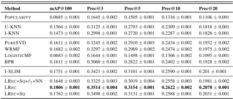
5.7.4 Results and analysis . . . 61
5.7.5 Long-tail recommendations . . . 63
5.7.6 Near cold-start recommendation . . . 63
5.7.7 Case-Study . . . 64
5.8 Experiments and evaluation of LINEAR-FLOWmodel . . . 65
5.8.1 Data description . . . 65
5.8.2 Evaluation protocol . . . 66
5.8.3 Model comparison . . . 66
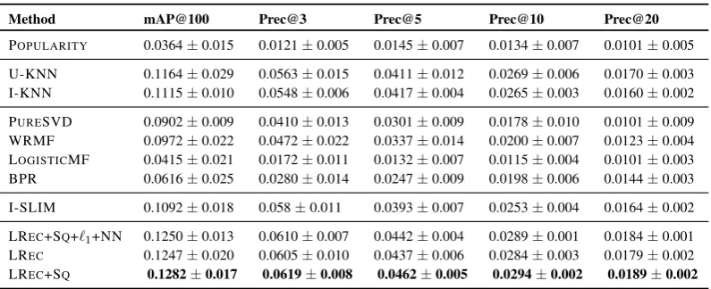
5.8.4 Results and analysis . . . 67
5.9 Conclusion . . . 70
6 Beyond Linear Models: Neural Architecture for Collaborative Filtering 71 6.1 Problem setting . . . 71
6.2 Background : Neural network architectures . . . 71
6.2.1 Restricted Boltzmann Machine (RBM) . . . 71
6.2.2 Autoencoders . . . 73
6.2.3 RBM for collaborative filtering (RBM-CF) . . . 73
6.3 AutoRec: Autoencoders meet collaborative filtering . . . 75
6.4 Relation to existing models . . . 76
6.4.1 Relation to matrix factorisation . . . 77
6.4.2 Relation to LRec and LINEAR-FLOW . . . 77
6.4.3 Relation to LoCo . . . 78
6.5 AutoRec for OC-CF . . . 78
6.6 Experiments and evalution . . . 78
6.6.1 Data description . . . 78
6.6.2 Model comparison . . . 79
6.6.3 Results and analysis . . . 79
6.7 Conclusion . . . 81
7 Conclusion 83 7.1 Summary of Contributions . . . 83
7.2 Future work . . . 84
7.2.1 Exploration of emerging deep learning architectures . . . 84
7.2.2 Incorporating temporal information . . . 84
7.2.4 Models for location aware recommendation . . . 85 7.3 Conclusion . . . 85
Appendix A Randomised SVD 87
List of Figures
2.1 Overview of recommender systems. . . 8
2.2 Feature encoding in Matchbox model. . . 11
2.3 Aggregation of social features. . . 16
3.1 Overview of Social Affinity Filtering setting. . . 22
3.2 Overview ofInteractionsandActivitiesin Facebook social network. . . 23
3.3 Training data for SAF. . . 26
3.4 Evaluation of SAF with baselines. . . 29
3.5 Cold-start evaluation of SAF . . . 30
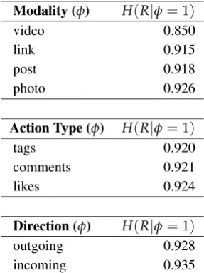
3.6 Conditional Entropy of modalities/activities . . . 31
3.7 Evaluation of informativeness of social affinity features. . . 34
3.8 Average conditional entropy of activities cumulative over the size. . . 34
3.9 Conditional entropy of favourites features. . . 35
3.10 Comparison of Accuracy of SAF with user activities. . . 35
3.11 Comparison of Accuracy of SAF with the number of active features. . . 35
4.1 Performance of COS-COSwith the number of page likes. . . 49
4.2 Performance of LoCo with the number of page likes. . . 49
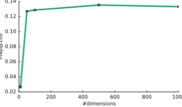
4.3 Performance of LoCo performance with the dimension of projection. . . 50
5.1 Long-tail results for LRec on ML1M dataset. . . 63
5.2 Improvement in Prec@20 of LRec over WRMF. . . 64
5.3 Performance of LRec with the number of training ratings. . . 64
5.5 Evaluation of recommendation of LRec and WRMF . . . 65
6.1 Restricted Boltzmann Machine. . . 72
6.2 Autoencoder model. . . 73
6.3 RBM based collaborative filtering model. . . 74
6.4 AUTORECmodel. . . 76
6.5 Generalised neural architecture for CF. . . 77
6.6 Performance of I-AUTORECon ML1M wrt number of hidden units. . . 81
List of Tables
1.1 Summary of the proposed methods . . . 4
3.1 Commonly used symbols for Social Affinity Filtering. . . 22
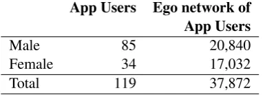
3.2 LinkR app users demographics. . . 27
3.3 Statistics on user interactions. . . 27
3.4 Statistics on user actions. . . 27
3.5 Dataset breakdown based on friend and non-friend link. . . 28
3.6 Conditional entropy of various interactions. . . 31
3.7 Most and Median informative favourite features. . . 33
4.1 Comparative overview of various cold-start methods . . . 41
4.2 Summary of cold-start recommendation for various approaches. . . 44
4.3 Description of Kobo and Flickr datasets. . . 45
4.4 Performance of generalised neighbourhood based cold-start model onKobodataset. . . . 47
4.5 Performance of generalised neighbourhood based cold-start model onKobodataset. . . . 47
4.6 Comparison of Cos-Cos cold-start model for various user side-information. . . 47
4.7 Comparison of cold-start recommenders onKobodataset. . . 48
4.8 Comparison of cold-start recommenders onFlickrdataset. . . 48
4.9 Performance of cold-start and near cold-start recommenders onKobodataset. . . 48
4.10 Comparison of validation times onKobodataset. . . 49
5.1 Comparison of recommendation methods for OC-CF. . . 54
5.2 Summary of datasets used in evaluation. . . 59
5.3 Results on ML1M dataset. . . 61
5.4 Results on LASTFM dataset. . . 61
5.5 Results on KOBOdataset. . . 62
5.6 Results on MSDdataset. . . 62
5.7 Comparison of LRec and WRMF recommendations . . . 65
5.8 Summary of datasets used in evaluation. . . 66
5.9 Results on ML10M dataset . . . 67
5.10 Results on LASTFM dataset . . . 67
5.11 Results on KOBOdataset . . . 67
5.12 Results on PROPRIETARY-1 dataset. . . 68
5.13 Results on PROPRIETARY-2 dataset. . . 68
5.14 Results on ML10M dataset. . . 69
5.15 Training time of various OC-CF methods. . . 69
5.16 Top-5 similar items learned by I-LINEAR-FLOWmodel. . . 70
6.1 Generalised AutoRec model. . . 77
6.2 Summary of datasets used in evaluation. . . 79
6.3 Comparison of AUTORECand RBM-CF models. . . 79
6.4 Performance of various optimization methods. . . 80
6.5 Variation of performance with the choice of activation functions. . . 80
6.6 Evaluation of AUTORECwith baselines. . . 81
List of Symbols
R Real number
R Partially observed user-item preference matrix
|R| Number of observed entries in matrixR
ˆ
R Recommendation matrix
U Set of users
I Set of items
XU Users’ side information XI Items’ side information
Iu Set of items purchased/rated by the useru Ui Set of users who purchased/rated the itemi A User latent factor matrix
B Item latent factor matrix
S Similarity matrix
Chapter1
Introduction
1
.
1
Background: Personalised recommendation
Over the last decade, the Internet has evolved into a platform for large-scale online services such as Amazon, Netflix, Facebook, eBay, and Youtube. These services has transformed the way we communi-cate, buy products, watch movies, and listen to music. The number of items1offered by online services
is unprecedented and ever increasing. As a result, automated systems for item filtering, suggestion and discovery have become very relevant.
Recommender systems are the algorithms that facilitate personalised recommendation by learning users’ preferences from a database of their past actions. At a high level, recommender systems are the algorithmic counterpart of a smart personal assistant that finds relevant items on your behalf. On the one hand, recommender systems reduce individual effort in finding relevant items; on the other hand, they add immense business value to the service providers. Specifically, recommender systems help online services to increase their sales [Lee and Hosanagar, 2014] and user engagement. For instance, [Davidson et al., 2010] reported that recommendation accounts for about 60% of total video clicks from Youtube homepage. Hence, recommender systems are at the core of the online services, such as:
• Entertainment:Online services, such as Netflix [Gomez-Uribe and Hunt, 2015], Youtube [Davidson et al., 2010], Spotify, etc. extensively use personalised recommendation to deliver relevant content to the users. Netflix reported that recommendations account for 80% of the hours streamed [Gomez-Uribe and Hunt, 2015].
• E-commerce: Many online stores, such as Amazon [Linden et al., 2003], eBay [Zhang and Pennac-chiotti, 2013], use recommender systems to help customers to find relevant items. By exposing users to relevant items, recommender systems not only attract potential buyers but also convert site surfers to buyers.
• Social networks: Recommender systems are widely used in online social networks to help users in
exploring new social connections and relevant contents. Facebook [Backstrom and Leskovec, 2011] and Twitter [Gupta et al., 2013] use recommender systems to suggest friends, interesting posts and to serve relevant advertisements. Similarly, Linkedin, a popular professional social network, uses recommender systems [Amin et al., 2012] in suggesting relevant jobs, companies, and candidates for recruiters.
There are two main approaches to personalised recommendation: content-based filtering (CBF) [Pazzani and Billsus, 2007] and collaborative filtering (CF) [Resnick and Varian, 1997, Sarwar et al., 2001, Linden et al., 2003, Koren et al., 2009, Koren, 2010b]. CBF makes a recommendation leveraging user and item
1We use the term item to refer products, books, movies, music, videos, etc.
attributes. On the other hand, CF algorithms make a personalised recommendation by directly learning users’ preferences from user-item interaction data. CF algorithms are widely popular mainly due to their superior performance over CBF [Linden et al., 2003]. In this dissertation, we primarily focus on developing CF algorithms for the personalised recommendation.
In a real-world recommendation task, there arise various scenarios based on data sources and prob-lem setting. CF can be categorised into two different probprob-lem classes,explicit feedback CFandone-class CF, depending on the nature of the preference data.Explicit feedback CFconcerns predicting user’s ac-tual preferences from rating, or like/dislikes data. One-class CF (OC-CF)concerns suggesting relevant items to users from the data that consists of only positive preferences such as item purchase. On the other hand, different CF scenarios arise based on the recommendation settings. For instance,Cold-start CF refers to the scenario when we do not have any historical data about users or items. Similarly,Social-CF
involves leveraging users’ signals from social networks when such data is available. In this dissertation, we focus on formulating algorithms for the above CF scenarios.
1
.
2
Motivation: What is lacking in existing CF algorithms?
Recommender systems are a very active area of research in both industry and academia. Over the years, many CF algorithms have been proposed. In general, it is desirable to have a CF framework that is (1) applicable to wide range of recommendation scenarios, (2) learning-based, (3) amenable to convex optimisation, and (4) scalable2. However, there are several limitations to existing approaches which
limit their application.
Most existing work on CF focuses on Neighbourhood (KNN) and Matrix factorisation (MF) meth-ods. KNN algorithms [Herlocker et al., 1999, Bell and Koren, 2007, Sarwar et al., 2001, Linden et al., 2003] make recommendations by finding similar users or items. As a key limitation, KNN uses prede-fined similarity metric instead of learning directly from the data by optimising some objective function, and hence is unable to adapt to the characteristics of the data at hand. On the other hand, MF al-gorithms [Salakhutdinov and Mnih, 2008b, Koren et al., 2009] incorporate learning by factorising the user-item preference matrix in an optimisation framework. However, MF models are non-convex, and hence are susceptible to sub-optimal local minima. Recently, [Ning and Karypis, 2011] proposed SLIM, a constrained linear model for OC-CF with a convex objective. However, SLIM is not user-focused and involves constrained optimisation limiting its applicability on large scale datasets.
In addition to the above limitations, a key problem with the existing approaches is that there is no definite answer as to which CF model class works best for broad range of recommendation scenarios. For instance, CF algorithms, such as MF, are unable to make recommendations in cold-start scenar-ios. Furthermore, most of the work on social-CF extends existing CF algorithms to incorporate social signals [Ma et al., 2011b, Noel et al., 2012, Ma et al., 2009b, 2008b]. However, these models are not expressive enough to incorporate fine-grained social signals limiting the full exploitation of the available data.
In summary, the existing approaches have several limitations for a real world recommendation sce-nario. Hence, there is a need for a different approach to CF that addresses all key desiderata.
§1.3 Our approach to CF: Linear models and beyond 3
1
.
3
Our approach to CF: Linear models and beyond
As discussed in Section 1.2, the existing approaches to CF have several limitations. In this section, we discuss our approach to CF addressing all the above desiderata.
1.3.1 Linear models for recommendation
In this dissertation, we focus on investigating linear models, an underappreciated but promising area for recommendations that addresses all CF desiderata. We formulate a unified framework based on linear models for different CF scenarios.
Linear models [Nelder and Baker, 2004] are the most widely used method for various practical ma-chine learning problems. They have several desirable properties, as we will discuss shortly, which make them attractive for a broad range of problems. First, unlike neighbourhood methods, linear methods learn from data by minimising some objective function. Second, linear models facilitate the design ofconvex
objectives which ensure globally optimal solution. Third, they aresimpleandscalable, which is very desirable while building a large-scale system. For instance, linear regression has a closed-form solution, which can be exploited to scale recommendation to large datasets, as we will show in this thesis. Further, we will show that the formulation of CF problems as a linear model yields an embarrassingly parallel model i.e. one that can be learned without distributed communication during the optimisation. Fourth, linear models are theoretically well understood, and various efficient off-the-shelf optimisation tools and algorithms are available. Fifth, Linear models are highlyinterpretable. Interpretability of the model not only helps to understand and improve the model but also to explain the recommendations generated by the model. Especially, by explaining the recommendations, the system becomes more transparent, builds users’ trust in the system and convinces them to consume the recommended items [Vig et al., 2009].
1.3.2 Beyond linear models
In the last couple of years, nonlinear methods have gained a lot of attention due to impressive perfor-mance. In particular, deep learning has revolutionised many areas of machine learning, namely computer vision [Krizhevsky et al., 2012], natural language processing [Mikolov et al., 2013] and speech recog-nition [Hinton et al., 2012] . However, there has been very limited research in the application of deep learning for CF [Salakhutdinov et al., 2007]. In this dissertation, we identify CF as an auto-encoding problem and propose a general nonlinear neural network architecture for CF, bridging the core of the thesis to the deep learning literature.
1
.
4
Key contributions of dissertation
Before outlining the contributions of this dissertation, we first define the commonly used symbols. Let
Rdenote the user-item preference matrix,Xdenote the user features, andX(te)denote cold-start users
features. Further, letR ⇡ PkSkQTk andX ⇡ UkSkVTk be a singular value decomposition (SVD) of
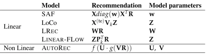
the preference and feature matrix respectively. Finally, let f(·),g(·)denote the activation function. The contributions of this dissertation are in formulating linear models for different CF scenarios and a neural architecture that generalises to various CF models. In this dissertation, we investigate various CF models as summarised in Table 1.1.
1. Linear models for social collaborative filtering
Model Recommendation Model parameters
Linear
SAF Xdiag(w)XTR w
LoCo X(te)V
kZ Z
LREC WR W
LINEAR-FLOW ZPTkR Z
[image:26.595.130.470.76.164.2]Non Linear AUTOREC f(U·g(VR)) U, V Table 1.1: Summary of the proposed models.
aggregates rich social information into a single measure of user-to-user interaction [Cui et al., 2011, Li and Yeung, 2009b, Noel et al., 2012, Ma et al., 2008b]. But in aggregating all of these interactions and activities into a single strength of interaction we discard valuable fine-grained information. Hence, the existing approaches to Social-CF are not capable of exploiting rich social data. To address this limitation, we propose a scalable linear Social-CF algorithm,Social Affinity Filtering (SAF), which learns to weight fine-grained user interaction and activities in a social network. We show that only a small subset of user interactions and activities are valuable for the recommendation, hence learning which of these are most informative is of critical importance. Furthermore, we show that Facebook page likes are highly predictive of users’ preferences. The insights from this work provide a foundation for the follow-up work on cold-start recommendation work.
2. Linear models for social cold-start recommendation
As a second contribution, we investigate linear models for cold-start recommendation. Without loss of generality, we focus on user cold-start3, for OC-CF setting. The user cold-start problem
concerns the task of recommending items to users who have not previously purchased or otherwise expressed preferences towards any item under consideration. We show how several popular cold-start models can be seen as special case of a linear content-based model. Leveraging this insight and the predictive power of social information, we propose a class of large-scale linear models that leverages high dimensional social information for the cold-start recommendation. We present a comprehensive experimental evaluation to demonstrate the superior performance of proposed method and the predictive power of social network content in addressing the cold-start problem.
3. Linear models for one class collaborative filtering
As a third contribution, motivated by the superior performance of the linear models on Social-CF and Cold-Start recommendation, we investigate linear models in a general OC-Social-CF setting. We propose, LREC, a user-focused linear model. LRECproduces user-personalised recommendations by training a convex, unconstrained objective that is embarrassingly parallelisable (i.e., without distributed communication) across users. A comprehensive set of experiments on a range of real-world datasets reveals LRecs superior performance compared to the state-of-the-art methods.
4. Large scale linear models via dimensionality reduction
Linear methods, LRec and SLIM, yield good performance on OC-CF problem. However, they involve solving a large number of regression subproblems, which can be impractical to large scale problems. Furthermore, LRec is also expensive regarding the memory requirements. We address these limitations by proposing LINEAR-FLOW, which formulates OC-CF as a regularised linear regression problem that uses randomised SVD for fast dimensionality reduction. Through
§1.5 Outline of dissertation 5
extensive experiments on real-world datasets, we demonstrate that Linear-Flow achieves state-of-the-art performance as compared to other methods, with a significant reduction in computational cost.
5. Neural network architecture for collaborative filtering
As a final contribution, we take a departure from linear models by exploring deep learning models. We show that a particular neural architecture, an Autoencoder, can represent a broad range of CF models. We propose AUTOREC, a neural architecture, that generalises various CF methods. A comprehensive set of experiments on a range of real-world datasets reveals that AutoRec yields state-of-the-art results on the rating prediction problem.
To summarise, the core of this dissertation focus on formulating a unified approach to CF using linear models that performs well on various CF scenarios. We conclude by bridging the core of the dissertation to deep learning architecture, and leading the way for future research on applying deep learning models to CF.
1
.
5
Outline of dissertation
In this thesis, starting from a concrete, practically relevant scenario where linear models are useful, we progressively use the insights derived in the design of these models to apply them to a broad spectrum of CF tasks.
Chapter 2 introduces the necessary background and terminology for recommender systems. In par-ticular, we introduce the terminologies and basic concepts. We discuss related work and seminal CF algorithms for different CF scenarios.
In Chapter 3, we introduce our novel Social collaborative filtering algorithm, Social Affinity Filtering (SAF). We provide a detailed experimental analysis and demonstrate the superiority of the proposed algorithm compared to state-of-the-art social collaborative filtering algorithms. Furthermore, we present feature analysis and demonstrate the substantial predictive power of social features.
In Chapter 4, we introduce our cold-start algorithm, LoCo, that leverages high dimensional social features. We present the experimental evaluation to demonstrate the superiority of proposed model and predictive power of social network content in addressing the cold-start problem.
In Chapter 5, we present LRec, a novel user focused linear model for one-class collaborative filtering. We perform a thorough experimentation on four real-world datasets to demonstrate the superiority of the LRec. Next, we address the computational and space limitation of LRec by proposing LINEAR -FLOW, a linear algorithm that leverages fast dimensionality reduction via randomised algorithms. In a comprehensive set of experiments, we show the proposed method is computationally efficient and yields comparable results.
Chapter 6 introduces AUTOREC, a general neural network architecture for CF. We report our evalu-ations on three different datasets and demonstrate that AutoRec yields the state-of-the-art results.
Chapter2
Overview of Recommender Systems
In this Chapter, we will formally define the recommendation problem, discuss approaches to the rec-ommendation and various Collaborative Filtering (CF) algorithms as outlined in Figure 2.1. We then discuss the four prevalent CF scenarios that we investigate in this dissertation, as mentioned in Chapter 1. We conclude by discussing evaluation metrics used in this dissertation to evaluate all recommendation algorithms.
2
.
1
Recommendation problem: Formal definition
Recommendation is essentially a task of predicting users’ preferences on items they have not consumed. Let U denote a set of users, and I a set of items, with m = |U| and n = |I|. Let R denote the observed user-item preference matrix; for explicit feedback R 2 Rm⇥n where higher scores refer to higher preference e.g. as in ratings, whereas forone-class feedback data R 2 {0, 1}m⇥n where R
ui
indicates whetherupurchased itemior not. For simplicity, we set the unobserved entries,Rui, to0. Let Iu denote the set of the items for which useruhas expressed preference, andUi be the set of the users
who have expressed preference for the itemi.
The goal of recommender systems is to predict the preferences of useruon unobserved items, i.e.
I Iu. In other words, recommendation can be defined as learning Rˆ 2 Rm⇥n, the recommendation
matrixwhich approximates users preference on items. We refer to the symbol table at the beginning of this dissertation for commonly used symbols. Formally, the recommendation problem is defined as:
Definition 1. Given a set of usersUand itemsI, a recommender system learns a functionF:Rm⇥n ! Rm⇥n, whereF(R) = Rˆ , which predicts users preference on items. Optionally, it can take any
addi-tional information, such as user featuresXU 2Rm⇥dor item featuresXI 2Rn⇥d
Based on the problem formulation and its evaluation, which we will discuss later, recommendation can be grouped into two different tasks:
• Rating Prediction taskconcerns with predicting the exact rating for user u on item i. Rating
prediction is exemplified by the Netflix challenge [Bennett et al., 2007b] and widely used in the explicit feedback setting.
• Ranking taskconcerns with recommending a ranked list of relevant items to a useru. Since the
end goal of a recommender system is to suggest a list of relevant items, recommendation as a ranking task is preferred in real world setting.
Recommendation Approaches
Collaborative Filtering (CF)
Matrix Factorisation (MF) Neighborhood (KNN)
Item-KNN User-KNN
Content Based Filtering (CBF)
Item-CBF User-CBF
Figure 2.1: Overview of recommender system approaches and models.
2
.
2
Approaches to recommendation
There are two main approaches to personalised recommendation, namelyContent based filteringand
Collaborative filtering.
2.2.1 Content based filtering (CBF)
Content-based filtering (CBF) [Pazzani and Billsus, 2007] uses item or user features 1 to predict the
users’ preferences. CBF treats the recommendation as regression or classification problem and learns a user or item specific recommendation model. There are two categories of CBF:
• User-CBFmakes a recommendation by learning an item-specific model from the user features
and observed preference for the corresponding item. Principally, User-CBF makes a recommen-dation by finding the items liked by the users with similar features. User demographics (age, sex, location, etc.) are widely used features for User-CBF.
• Item-CBFlearns a user-specific recommendation model from the item features and observed pref-erence for the corresponding user. Item descriptions, tags, and reviews are widely used item fea-tures for Item-CBF.
CBF has some advantages, especially forcold-startrecommendation i.e. they can provide meaning-ful recommendation to the users without any preference data. However, the key limitation of CBF is that they suffer from over-specialization [Lops et al., 2011], which means the recommended items lack novelty. For instance, the recommendation for Item-CBF is restricted to the items that are similar to the previously liked items. Similarly, the recommendations for User-CBF are limited to the items liked by similar users based on a coarse approximation from the users’ features. Hence, CBF lack serendipitous discovery of items.
2.2.2 Collaborative filtering (CF)
Collaborative Filtering (CF) [Goldberg et al., 1992, Resnick and Varian, 1997, Sarwar et al., 2001, Linden et al., 2003, Koren et al., 2009, Koren, 2010b] is the most popular recommendation algorithm and has become the de facto choice of model for recommendation. CF algorithms are based on the general idea that users’ preferences may be correlated and one can detect and exploit these correlations across
§2.3 Collaborative filtering models 9
the user population to make recommendations for a user. In a broad sense, CF algorithms leverages three different kinds of correlation within the user-item preference data:
• inter-item correlation, which refers to the fact that the items liked by similar set of users are
correlated
• inter-user correlation, which refers to the fact that the user who liked similar set of items are
correlated
• intra user-item correlation, which refers to the fact that the users who agreed in the past will tend
to agree in the future. Similarly, users tend to prefer the items that are similar to the ones they already liked.
Based on these key assumptions, CF algorithms exploit the wisdom of the crowd by predicting users’ preferences not only from her past actions but also from the preferences of like-minded users. In other words, CF algorithms allows users to collaborate with each other in predicting user’s preferences.
Over the years, many CF algorithms have been proposed. Tapestry [Goldberg et al., 1992] was the first system to introduce the term CF and applied it in the context of email filtering. Later, [Resnick et al., 1994] proposed a rating based CF system for recommending news articles. Although CF had been an active area research in industry, it received lots of attention after the “Netflix challenge“ [Bennett et al., 2007b].
CF algorithms are attractive for recommendation due to various reasons. First, CF learns to make personalised recommendation from preference data. Second, unlike CBF, CF algorithms do not over-specialize and are capable of makingserendipitous[Herlocker et al., 2004] recommendations. However, most of the CF algorithms are not capable of making recommendations in cold-start scenarios. In the following section, we will discuss various CF algorithms in detail.
2
.
3
Collaborative filtering models
In this section, we discuss the various types of CF algorithms.
2.3.1 Neighbourhood models (KNN)
Neighbourhood-based CF models [Herlocker et al., 1999, Bell and Koren, 2007, Sarwar et al., 2001, Linden et al., 2003] are based on the general idea that users share their taste with similar users or similar items. Neighbourhood-based CF makes recommendations by computing k-nearest neighbours for each user or item. Hence, it is referred as k-Nearest Neighbour (KNN) algorithm in the literature. KNN based CF defines neighbourhood from observed user-item preference data using various predefined similarity metrics, which we will discuss shortly. There are two approaches to neighbourhood-based models:
1. User-Based Neighbourhood Model (U-KNN) [Herlocker et al., 1999, Bell and Koren, 2007] leveragesinter-userandintra user-itemcorrelation from the observed user-item preference data. It is based on the key assumption that the similar users like similar items and predicts users’ preferences using the user-user similarity matrix.
2. Item-Based Neighbourhood Model (I-KNN)[Sarwar et al., 2001, Linden et al., 2003] leverages
Various similarity metrics are used to define the neighbourhood. The most common similarity met-rics are
Pearson Correlation, which measures the strength and direction of the linear relationship between entities. For rating data, Pearson correlation between usersuandvis computed as
Suv= Âi2Iuv(Rui
¯
Ru)(Rvi R¯v) q
Âi2Iuv(Rui R¯u)2
q
Âi2Iuv(Rvi R¯v)2
where, Iuv = Iu\Iv, and Ru¯ and Rv¯ are the mean of the observed ratings for user u and v
respectively.
Cosine Similarity, which measures the angle between two vectors. It is widely used in both rating prediction and item recommendation problem. The cosine similarity between user u and v is computed as
Suv= hRu:,Rv:i
kRu:k2kRv:k2, whereh·,·idenotes inner product.
Jaccard Similarity, which measures the similarity between two sets. The Jaccard similarity between useruandvis computed as
Suv= |Iu\Ii|
|Iu[Ii|
The similarities between itemsSijcan be computed in a same way.
Neighbourhood methods are attractive for several reasons. They are simple to implement, efficient, and interpretable. However, they defineS using a fixed similarity metrics instead of learning them by optimising some principled loss function [Koren, 2008]. Further, recommendation performance can be quite sensitive to the choice ofS, and the choice depends on the problem domain(as shall be shown in later experiments). Hence, neighbourhood methods are unable to adapt to the characteristics of the data at hand.
2.3.2 Matrix factorisation models (MF)
MF based models [Srebro and Jaakkola, 2003, Salakhutdinov and Mnih, 2008b, Koren et al., 2009] embed users and items into some shared latent space, with the aim of inferring complex preference profiles for both users and items. MF models are based on the key idea that the user-item preference data is correlated, and hence can be expressed in terms of low-rank user and item latent factors.
Formally, letJ 2 Rm⇥n+ be some pre-defined weighting matrix to be defined shortly. Let`: R⇥ R ! R+be some loss function, typically squared loss`(y, ˆy) = (y yˆ)2. Then, the general matrix
factorisation framework optimises
min
§2.4 Collaborative filtering scenarios 11 0 1 0 2 0 3 1 4
· · · 0
m 2 0 m 1 0 m 1
m+1
0
m+1
· · · 0
m+du 1
1
m+du
one-hot encoding for useru4 u4features
Figure 2.2: XUfor useru
4in matchbox model
where the recommendation matrix is2
ˆ
R(q) =ATB (2.2)
forq ={A,B}, andW(q)is theregulariser, which is typically
W(q) = l
2 ·(||A||2F+||B||2F)
for somel> 0. The matricesA2 Rk⇥m,B 2Rk⇥nare thelatent representationsof users and items respectively, withk2N+being thelatent dimensionof the factorisation.
MF is one of the most extensively studied model in the field of CF. [Salakhutdinov and Mnih, 2008a] proposed a fully Bayesian model for MF. Similarly, [Lawrence and Urtasun, 2009] proposed a nonlinear MF algorithm using Gaussian process. However, these models are computationally expensive and are not suitable for large scale recommendation.
Further, there have been extensions of MF to incorporate user and item side information such as [Stern et al., 2009] , which we refer as Matchbox model. Matchbox defines the recommendation matrix as
ˆ
R(q) = (AXU)T(BXI) (2.3)
where, A 2 Rk⇥(m+du), B 2 Rk⇥(n+di), XU 2 R(m+du)⇥m, and XI 2 R(n+di)⇥n. Here, XU composed of users features and one-hot encoding of the user index as shown in Figure 2.2. Similarly,XI
composed of item features and one-hot encoding of the item index. Intuitively, Matchbox embeds the user and item side information to thekdimensional latent space. Matchbox corresponds to MF model if only one-hot encoding of user and item indices are used as features.
One of the fundamental limitation of MF based methods is that the problem is non-convex, hence susceptible to local minima. Furthermore, the recommendations are based on latent factors and are not easily interpretable [Zhang et al., 2014] as in neighbourhood methods.
2
.
4
Collaborative filtering scenarios
In a real-world recommendation task, there arise various scenarios based on data sources and problem setting. In this dissertation, we discuss four prevalent scenarios, as discussed in Section 1.1:
2.4.1 Explicit feedback CF
Explicit feedback CF concerns with the prediction of users’actualpreferences such as rating, like/dislikes. From here onwards, we use the term“rating”to refer explicit feedback. We discuss various CF models for explicit feedback scenarios :
KNN models
User-based KNN [Herlocker et al., 1999, Bell and Koren, 2007] defines the rating prediction as weighted sum of the ratings given by users’ neighbours.
ˆ
Rui = Âv2Nk(u,i)Suv(Rvi bvi) Âv2Nk(u,i)Suv
(2.4)
whereNk(u,i)is the set of k-nearest neighbours, as defined byS, of useruwho have rated the itemi.
Item-based KNN[Sarwar et al., 2001] defines the rating prediction as weighted sum of the rating of the similar items.
ˆ
Rui = Âi2N
k(u,i)Sij(Ru,j buj)
Âj2Nk(u,i)Sij
(2.5)
whereNk(u,i)is a set of k-nearest neighbour of itemiwhich is rated by the useru.
MF models
For rating prediction [Salakhutdinov and Mnih, 2008b, Koren et al., 2009], one typically sets Jui =
JRui > 0Kin equation 2.1 , so that one only considers (user, item) pairs with known preference
infor-mation. The MF model [Salakhutdinov and Mnih, 2008b] for rating prediction optimises
min
A,B u2U
Â
i,i2Iu
(Rui ATuBi)2+l2(||A||2F+||B||2F) (2.6)
Additionally, biased matrix factorisation (Biased-MF) [Koren et al., 2009] incorporates a global, user, and item bias by optimising
min
A,B u2U
Â
i,i2Iu
(Rui b bu bi ATuBi)2+ l2(||A||2F+||B||2F), (2.7)
whereb, bu, bi are global, user and item bias respectively.
Most recently, [Lee et al., 2013] proposed Local Low Rank Matrix Factorisation (LLORMA), an ensemble MF algorithm that minimises the squared error weighted by the proximity of user-item pair to a predefined point called anchor point. Formally, it minimises
min
A,B (u⇤
Â
,i⇤)2QK((u,i),(u⇤,i⇤))(Rui AT
uBi)2+l2(||A||2F+||B||2F), (2.8)
whereK((u,i),(u⇤,i⇤))is a two-dimensional smoothing kernel that measures the proximity of tar-get point(u,i)to the anchor point(u⇤,i⇤);Qis a set of anchor points. In general, it learns local matrix
factorisation model with respect to each anchor point. Finally, givenqdifferent anchor points, the rating is estimated as a linear combination of predictions from each model.
2.4.2 One-class CF
§2.4 Collaborative filtering scenarios 13
the term “purchase” to refer one-class feedback in general. We discuss various CF models for OC-CF scenarios :
KNN models
User-based KNNpredicts the users’ preferences on items as:
ˆ
Rui =
Â
v2Nk(u,i)Suv (2.9)
whereNk(u,i)is a set of k-nearest neighbour of useruwho also purchased the itemi. Item-based KNN[Linden et al., 2003] predicts the users’ preferences on items as:
ˆ
Rui =
Â
j2Nk(u,i)Sij (2.10)
whereNk(u,i)a set of k-nearest neighbour of itemithat are purchased by useru.
Note that unlike rating prediction(as in Equation 2.4 and 2.5), we do not normalise the score. This is mainly because we are concerned with the relative scores in OC-CF setting.
Sparse Linear Methods (SLIM)
As an alternative to neighbourhood methods for OC-CF, Sparse linear Methods (SLIM) [Ning and Karypis, 2011] directly learns an item-similarity matrixW 2Rn⇥nvia
min
W2C||R RW|| 2
F+l2||W||2F+µ||W||1 whereC={W2 Rn⇥n: diag(W) =0,W 0},
(2.11)
wherel,µ > 0are appropriate constants. Here, || · ||1denotes the elementwise `1 norm of W so as to encourage sparsity, and the constraint diag(W) = 0prevents a trivial solution ofW = In⇥n. The
nonnegativity constraint encourages interpretability, but Levy and Jack [2013] demonstrated that good performance can be achieved without it. Given a learnedW, SLIM produces a recommendation matrix
ˆ
R(q) =RW.
Thus, SLIM is equivalent to an item-based neighbourhood approach where the similarity matrix
S= Wislearnedfrom data. Although SLIM has a convex learning objective, it is item-focused which hampers it predictive performance. Similarly, it involves constrained optimisation, which limits fast training.
MF models
For OC-CF, we cannot set the weighting matrix Jui = JRui > 0K for MF objective shown in
equa-tion 2.1, as one will simply learn on the known positive preferences, and thus predict Rui = 1. An
alternative is to setJui =1uniformly. This treats all absent purchases as indications of a negative
As an intermediate between the two extreme weighting schemes above, the WRMF method [Pan et al., 2008, Hu et al., 2008] setsJuito be
Jui =JRui =0K+a·JRui >0K (2.12)
where a assigns an importance weight to the observed preferences. WRMF uses Alternating Least
Squares (ALS) method for optimization. The solution for Aand B in each step of ALS is given by (2.13)
A:u = (BJUBT+lI) 1BJURTu:
B:i = (AJIAT+lI) 1AJIR:i
(2.13)
whereJU 2 Rn⇥n andJI 2 Rm⇥m are diagonal matrices such thatJU
ij = Jui andJuuI = Jui. In each
iteration of ALS, due to the weighting, we need to compute the inverse for each user and item as shown in (2.13). This makes WRMF computationally expensive compared to using uniform weights.
[Tang and Harrington, 2013] proposed a randomised SVD based method to scale uniformly weighted MF for OC-CF on large-scale datasets. The proposed method involves computation of rank-k ran-domised SVD of the matrixR(as discussed in Appendix A).
R⇡PkSkQTk (2.14)
wherePk 2 Rm⇥k,Qk 2 Rn⇥k andSk 2 Rk⇥k. Given the truncated SVD solution, they initialize the
item latent factor with the SVD solution and solve
argmin
A R A
TB 2
F+lkAk
2
Fs.t.B=S
1 2
kQTk (2.15)
Similarly, if the matrixAis fixed instead of the matrixB, the objective becomes
argmin
B R A
TB 2
F+lkBk
2
Fs.t.A=PkS
1 2
k (2.16)
We refer to (2.16) and (2.15) as U-MF-RSVD and I-MF-RSVD respectively.
Bayesian Personalised Ranking (BPR)
An alternate strategy to adapt matrix factorisation techniques to the OC-CF is theBayesian Personalised Ranking (BPR)Rendle et al. [2009]. BPR optimises a loss over (user, item) pairs, so as to ensure that the known positive preferences score at least as high as the unknown preferences:
min
q u2U,i2R
Â
(u),i02/R(u)
`(1, ˆRui(q) Rˆui0(q)) +W(q), (2.17)
where`(1,v) =log(1+e v)is the logistic loss, andRˆ is as per Equation 2.2. Intuitively, this forces
§2.4 Collaborative filtering scenarios 15
optimisation is feasible; nonetheless computational complexity remains a concern with such pairwise ranking approaches.
Gantner et al. [2012] proposed an extension of BPR that normalises the loss for each user,
min
q u
Â
2U,i2R(u),i02/R(u) 1
|R(u)| ·`(1, ˆRui(q) Rˆui0(q)) +W(q).
This can be seen to be more appropriate than Equation 2.17 in scenarios where we want to ensure good recommendations for the average user, i.e. the model is user-focused.
2.4.3 Cold-start CF
Cold-start problem [Schein et al., 2002] refers to the scenario when we do not have any historical pref-erence data about the users or items under consideration for recommendation. This proves a challenge for CF algorithms that explicitly rely on such information to make personalised recommendations. In such scenarios, user and item side information [Zhang, Zi-Ke et al., 2010, Sahebi and Cohen, 2011, Ma et al., 2008a, Cao et al., 2010, Jamali and Ester, 2010, Krohn-Grimberghe et al., 2012] are leveraged to make personalised recommendation.
Formally, in a standard cold-start setting, we have set of users with historical preference data,U(tr)
, referred aswarm start users, and targetcold-start usersU(te). LetX2 Rm⇥drefer to user metadata,
andX(tr),X(te)be the metadata for the warm- and cold-start users respectively. There are two classes of
model that leverages side-information for cold-start recommendation:
Neighbourhood based cold-start CF
Neighbourhood based cold-start CF [Zhang, Zi-Ke et al., 2010, Sahebi and Cohen, 2011] uses metadata to compute user-user or item-item similarity, and makes recommendation as discussed in 2.3.1. We will discuss the neighborhood based cold-start CF in detail in Chapter 4.
MF based cold-start CF
MF based cold-start CF [Krohn-Grimberghe et al., 2012] borrows the idea from collective matrix fac-torisation (CMF) [Singh and Gordon, 2008] for cold-start recommendation and optimises
min
A,B,Z||R AB||
2
F+µ||X AZ||F2+lA||A||2F+lB||B||2F+lZ||Z||2F (2.18)
whereA 2 Rm⇥k,V 2 Rk⇥n, and Z 2 Rk⇥d for somelatent dimensionalityk ⌧ min(m,n). The
intuition for this approach is that it finds a latent subspaceAfor users that is jointly predictive of both their preferences and social characteristics. We then predict
ˆ
R(te) =A(te)B. (2.19)
Another popular cold-start approach is the two-step modelBPR-LinMap[Gantner et al., 2010]. Here, the first step is to model the warm-start users byR(tr) ⇡A(tr)B, with latent featuresA(tr),Bas before.
The second step is to learn a mapping between the metadata X(tr) and latent features A(tr) using e.g.
linear regression,
A(tr)
u
v
m
m
S
Friendship Graph
S
Message GraphS
Tag GraphS
Like Graphu
v
m
m
S
socFigure 2.3: Aggregation of the social features.
forT2Rd⇥k. We then estimate the cold-start latent featuresA(te) =X(te)T, and use Equation 2.19 for
prediction.
2.4.4 Social CF
Social-CF is an emerging field in recommender systems research. Social-CF concerns about leverag-ing social signals from online social networks for a recommendation. The fundamental assumption in Social-CF is that users’ choices are not only influenced by personal preferences but also by interpersonal factors, such as friend groups. Recent findings from social science research also reinforce the impor-tance of social influence in user preferences. For insimpor-tance, [Brandtzg and Nov, 2011] found that the real-world interactions correlate with the strength of ties while virtual interactions reveal interest. Sim-ilarly, people who interact frequently tend to share similar interests [Singla and Richardson, 2008] and level of user interactions correlate with the positive ratings that they give each other [Anderson et al., 2012].
The signals from online social networks range from simple user-user interaction to complex rela-tions and interacrela-tions. In general, social networks are composed of two components, theSocial graph, which consists of user-user relationship, such as friendship, and the Interest graph, which consists of user preferences and interests such as page likes, group membership. In general, Social-CF extends MF model and leverages user-user social relation,Ssoc2Rm⇥m, defined by aggregating different social
sig-nals. In Figure 2.3, we show aggregation of social signals intoSsocfrom various user-user social signals,
such asSFriendship Graph, which refers to user-user friendship relationship;SMessage Graph, which refers
to the communication graph;STag Graph, which indicates whether users are tagged in same photo; and SLike Graph, which indicates whether users have shared likes, i.e
Ssoc=F(SLike Graph,STag Graph,SMessage Graph, ...,SFriendship Graph) (2.21) whereFis some aggregation function. In general,Ssoc is incorporated in MF framework by adding a
§2.5 Evaluation of recommender systems 17
2009a] to MF objective. In other words,Lsocialacts as a regulariser to MF objective.
Lsocial= `(Ssocuv,A) (2.22)
For instance, [Ma et al., 2011a, Li and Yeung, 2009a] used friendship relation and definedLsoc
Lsocial=
Â
u v2Â
N(u)Ssocuv kAu Avk2
whereN(u)is a set of friends of useru.
As an alternative to social regularisation, [Ma et al., 2008a] formulated social recommendation as a co-factorisation problem
min
A,B
Â
u,i(Rui AT
uBi)2+
Â
u,v(Ssoc
uv ATuZi)2+ l2(||A||2F+||B||2F+||Z||2F) (2.23)
Similarly, [Ma et al., 2009a] proposed a model that predicts rating as a weighted average of users’ and her friends rating, and minimises
min
A,B
Â
u,i(Rui (aAT
uBi+ (1 a)
Â
v2N(u)ATvBi)2 (2.24)
Most recently, [Noel et al., 2012] proposed a social extension to Matchbox, as defined in Equation 4.5. We refer this model asSocial Matchbox (SMB). It optimises
min
A,B u2U
Â
i,i2Iu
(Rui (AxUu)T(BxiI))2+ l2S
Â
u,v(Ssoc
uv (AxUu)T(AxUv))2+l2A||A||2F+l2B||B||2F
(2.25) wherexU
u andxiI are the corresponding side-information, as shown in Figure 2.2, for the useruand
itemirespectively.
In general, the key limitation of existing Social-CF methods is that they do not leverage fine-grained social interactions. Instead, they useSsoc, an aggregation of all social signals into a single numeric value,
limiting the full exploitation of the available social data.
2
.
5
Evaluation of recommender systems
The evaluation of a model is of critical importance while developing machine learning systems. Evalua-tion allows to quantify the performance of the model. In general, there are two broad categories of model evaluation, namelyonlineandofflineevaluation. Online evaluation concerns with comparing different models in a production environment by directly collecting feedback from the users such as A/B testing. On the other hand, offline evaluation concerns with evaluating the models used the gathered data by dividing it into train and test set. Although online testing is desirable, it is expensive and most impor-tantly requires access to the production system. Hence, in this dissertation, we use offline evaluation to evaluate the models.
2.5.1 Error based metrics
Error based metrics evaluate the prediction accuracy, and are widely used to access the performance of recommender system for rating prediction. In this dissertation, we use the two most widely used metrics:
Mean Absolute Error (MAE) measures how close the predicted value is from the ground truth in magnitude
MAE(R, ˆR) = 1
|R|
Â
u,i|Rui Rˆui|where|R|is the number of observed entries inR.
Root Mean Square Error (RMSE)penalises large errors more compared to MAE. RMSE was popu-larised in recommender systems evaluation by the Netflix competition [Bennett et al., 2007b].
RMSE(R, ˆR) = s
1
|R|
Â
u,i(Rui Rˆui)22.5.2 Ranking metrics
Ranking metrics evaluates the quality of the recommended list, and are widely used to evaluate the per-formance of recommendation models. In this dissertation, we use the three most widely used ranking metrics: precision@k, recall@k, andmean Average Precision@k. Let, Irec
u be the sorted list of
recom-mended items for a useru.
Precision@kmeasures the fraction of relevant items in the top-k recommended list, and is defined as
precision@k(u) = |Iu\I rec u [:k]| k
precision@k=
m
Â
u=1precision@k(u) m
Recall@kmeasures the fraction of the relevant items that are present in the top-k recommended list, and is defined as
recall@k(u) = |Iu\Iurec[:k]|
|Iu|
recall@k=
m
Â
u=1recall@k(u) m
mean Average Precision@k (mAP@k)3is another widely used metric to evaluate recommender
sys-tems. Unlike precision@kandrecall@k,mAP@k considers ordering of the items in the recom-mended list by giving more importance to the item at the top of the list. Formally, it is defined
§2.6 Summary 19
as
ap@k(u) = k
Â
i=1precision@i(u) min(|Iu|,|Iurec[:i]|)
mAP@k=
m
Â
u=1ap@k(u)
m .
Mean average precision approximates the area under the precision-recall curve for each user [Man-ning et al., 2008].
2
.
6
Summary
Chapter3
Linear Models for Social
Recommendation
In this Chapter, we delve into Social Collaborative Filtering (Social-CF), one of the prevalent CF sce-narios, as discussed in Chapter 2. We highlight the limitations of the existing methods and formulate a novel Social-CF algorithm using linear models addressing the key limitations. The insights from this chapter will serve as a foundation for cold-start recommendation, another CF scenario, which we will discuss in the following chapter.
3
.
1
Problem statement
In this Chapter, we are concerned with predicting whether userulikes an itemior not. The historical preference data consist of explicit likes and dislikes i.e. we have partially observed user item preference dataR2{0, 1}m⇥n, where1indicates like and0indicates dislike. Further, we have rich social network
data of the corresponding users and their friends. Unlike the classical recommendation setting, such as movie recommendation, in many real world scenarios the items can be highly heterogeneous. For in-stance, Facebook recommends us the links liked by friends, where the link can be a hyper-link to videos, blog posts, and news articles. In such heterogeneous settings, the number of items for recommendation can be large, leading to thedata sparsityproblem. Hence, it is critical to leverage user side information. In this Chapter, we focus on formulating models that leverage users’ social network data.
3
.
2
Background
In this Chapter, we investigate Social-CF algorithms in the context of the Facebook social network. Online social networks such as Facebook record a rich set of user preferences (likes of links, posts, pho-tos, videos), user traits, interactions and activities (conversation streams, tagging, group memberships, interests, personal history, and demographic data). The availability of rich labelled graph of social inter-actions and contents presents a myriad of new dimensions to the recommendation problem. The users’ signals from a social network range from simple user-user signals to complex information that spans across the network. However, most existing Social-CF methods, as discussed in section 2.4.4, aggregate the rich fine-grained social signals into a simple measure of user-to-user interaction [Cui et al., 2011, Yang et al., 2011a, Ma et al., 2011a, Li and Yeung, 2009a, Noel et al., 2012]. But by aggregating all of these signals into asinglestrength of interaction, we discard rich fine-grained social signals, as we will show in this chapter. Further, the existing methods extend Matrix Factorisation (MF) models, which are inherently non-convex and hard to interpret, as discussed in Section 2.3.2.
Acronyms Meaning
SAF Social Affinity Filtering Algorithm
ISAF Interaction Social Affinity Features
ASAF Activity Social Affinity Features
Symbols Meaning
R User-Item preference data
X Users’ social signals (interactions/activities)
f Social Affinity Features
H Conditional Entropy
Table 3.1: Symbols and Acronyms used for Social Affinity Filtering.
In this work, we take a departure from the existing approaches and formulate a Social-CF algorithm,
Social Affinity Filtering (SAF), using convex linear models that directly leverages fine-grained social signals for the recommendation. Further, we will also show how leveraging social signals can mitigate the cold-start problem.
User%u%
Social%Affinity% Group%%
Link%i% Like?%
Like/Dislike% Interac:ons%
and% Ac:vi:es%
Interac:ons%
Ac:vi:es%
{link,%post,%photo,%video}%×%{like,%tag,%comment}%×%{incoming,%outgoing}
%
Groups% Pages% Favourites%
Figure 3.1: A typical recommender system uses only ”like/dislike” data for recommendation, whereas, social recommender systems seek to leverage users’ social network data to predict their preferences.
3
.
3
Social affinity filtering
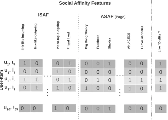
In this section, we define various social signals and social features, namelysocial affinity features. We then formulate Social-CF as a linear classification problem,Social Affinity Filtering (SAF), that leverages fine-grainedsocial affinity features. The key idea behind SAF is that the fine-grained social signals are predictive of users’ preferences. For instance, useruwho has likedJustin Bieber Facebook pagemight have similar taste as otherJustin Bieberfans. Now, we proceed to formalisingSocial Affinity Filtering (SAF). In Table 3.1, we summarise the additional symbols and acronyms defined in this chapter.
3.3.1 Social signals
In this work, we define two different types of social signals in a social network. We use the term