Analysis of the singular value decomposition as a tool for processing microarray expression data

pp. 250–259

ANALYSIS OF THE SINGULAR VALUE DECOMPOSITION AS A TOOL FOR PROCESSING MICROARRAY EXPRESSION DATA

DESMOND J. HIGHAM∗_{, GABRIELA KALNA}†_, AND J. KEITH VASS‡

Abstract. We give two informative derivations of a spectral algorithm for clustering and par-titioning a bi-partite graph. In the first case we begin with a discrete optimization problem that relaxes into a tractable continuous analogue. In the second case we use the power method to derive an iterative interpretation of the algorithm. Both versions reveal a natural approach for re-scaling the edge weights and help to explain the performance of the algorithm in the presence of outliers. Our motivation for this work is in the analysis of microarray data from bioinformatics, and we give some numerical results for a publicly available acute leukemia data set.

keywords: bioinformatics, clustering, data mining, microarray, power method, singular vaue decomposition.

AMS:92D10, 92C55, 65F15

1. Introduction. Microarray technology gives information about the expression levels of thousands of genes simultaneously. When microarray data from a number of samples is collected, the natural data structure is a bi-partite graph with non-negatively weighted edges. An important problem is then to partition, or cluster, the graph in an attempt to produce sets of genes and sets of samples such that each set of genes behaves uniformly across each set of samples. Here, we give analytical and experimental support for the use of the singular value decomposition (SVD).

In the next section we motivate the problem. In section 3 we start with a discrete optimization problem and proceed by adding constraints and relaxing to the contin-uous setting. By breaking the derivation into transparent steps, we are able to gain insights into the potential performance of the algorithm. This analysis generalizes the work in [9] to the bi-partite graph case. In particular, we show that there is a natural, justifiable, way to pre-process the edge weights to account for differently callibrated genes or samples. In section 4 we give an alternative derivation. Here, the solution is expressed as the limit of an iterative procedure that updates the clustering values based on an easily interpreted rule that measures the relative connectedness of the data points.

In section 5 we apply the algorithm to some small scale, artificial test data in order to get a feel for the performance and visualize the output. In section 6 we then apply the algorithm to a microarray data set of acute leukemia published in [3] and [7] (http://www.broad.mit.edu/cgi-bin/cancer/datasets.cgi) and interpret the results biologically.

2. Spectral Bi-Clustering. We are concerned with the case where a number of microarray samples have been generated for a common set of genes [1], [2], [7]. Typically, samples correspond to different pieces of tissue. For each gene in each sample, we suppose that a non-negative weight has been recorded to quantify the activity of the gene in that sample. If there are M genes and N samples, then

∗_{Department of Mathematics, University of Strathclyde, Glasgow G1 1XH, UK. Supported by a}

Research Fellowship from the Royal Society of Edinburgh/Scottish Executive Education and Lifelong Learning Department and by EPSRC grant GR/S62383/01.

†_{Department of Mathematics, University of Strathclyde, Glasgow G1 1XH, UK.} ‡_{Beatson Institute for Cancer Research, Glasgow G61 1BD, U.K.}

a rectangular matrix W _{∈ R}M×N _{stores the weights, with w}

ij ≥0 representing the

activity of theith gene in thejth sample. This data fits into the general framework of anon-negatively weighted bi-partite graph—nodes can be split into two groups (genes and samples) such that a weighted edge exists only for pairs of nodes in distinct groups.

The matrixW is normally long and thin; values such asM _≈30,000 genes and

N _≈100 samples are typical. In trying to find easily-summarized structure in the dataset, a reasonable approach is to bi-cluster simultaneously the genes and samples; that is,

to partition the genes into two distinct groups, Aand B, and simi-larly, partition the samples into two distinct groups,AbandBb, where genes in groupAtend to be active in samplesAband inactive in sam-plesBb, and similarly, genes in groupB tend to be active in samples

b

B and inactive in samplesAb.

The biological motivation behind a search for this pattern is that genes involved in a common function should be active in a common set samples. Revealing this structure provides information about sets of genes that take part in a common process and about samples in which such a process takes place.

This bi-clustering goal has been considered in [11], where justification is given via existing microarray datasets. Kluger et al. propose the singular value decomposition (SVD) as a means to bi-cluster, and our main aim here is to provide further theoretical support and algorithmic insight into the use of the SVD in this respect.

We will focus throughout on the microarray application and refer to ‘genes’ and ‘samples’, but we emphasize that the analysis here is quite general and applies to any bi-partite graph with weighted edges; in particular, very similar problems arise in related areas of bioinformatics and in other data mining applications [4], [8], [12], [14].

3. Optimization Viewpoint. Let pi ∈ {−21,12} be an indicator vector

com-ponent that determines whether gene i is placed in group A or B. Similarly, let

qj ∈ {−12, 1

2}be an indicator vector component that determines whether samplej is

placed in groupAborBb. Consider first the problem

min

M

X

i=1 N

X

j=1

(pi−qj)2wij.

(3.1)

Here, we seek to minimize the sum of the weightswij that relate non-matching genes

and samples. To avoid the trivial solution where all genes/samples are put into a single group (with the other group remaining empty), we add the constraints

M

X

i=1

pidgene_i ≈0 and N

X

j=1

qjdsample_j≈0,

(3.2)

where dgene_i := PNk=1wik is the total expression weight for gene i and dsample_j :=

PM

k=1wkj is the total expression weight for samplej. The constraints (3.2) make sure

that overall expression levels are roughly balanced across the two groups of genes and across the two groups of samples.

To reduce this discrete optimization task to a tractable problem, we look for a solution withp_∈RM _{and p}

p and q will have components that fall into distinct groups, and hence will reveal obvious partitions. This relaxation idea has been successfully used in a number of data mining applications [4]. After relaxing, to avoid the trivial solutionp_≡0 and

q_≡0 we impose the normalization constraints

M

X

i=1

p2idgene_i= 1 and N

X

j=1

qj2dsample_j= 1.

(3.3)

Constraints (3.3) damp down the influence of ‘promiscuous’ genes and samples, that is, genes and samples with large overall connectivity—a largedgenei ordsamplej value

encourages a pi or qj value close to zero. Having relaxed to real valued indicator

vectors, we may strengthen to exact equality in (3.2), giving

pTdgene=qTdsample= 0.

(3.4)

Letting Dgene = diag(dgene)∈RM×M andDsample= diag(dsample)∈RN×N, the

two-sum PM_i=1PN_j=1(pi−qj)2wij expands to pTDgenep+qTDsampleq−2pTW q and

hence the problem (3.1) under constraints (3.3) and (3.4) may be written

max{pTW q : p∈RM_{, q}

∈RN_{, p}T_d

gene=qTdsample= 0,

kD 1 2

genepk2=kD 1 2

sampleqk2= 1}.

(3.5)

Theorem 3.4 below solves this problem with the aid of Lemmas 3.1–3.3. First, we recall that any matrix A ∈ RM×N _{has SVD of the form A = UΣV}T_{, where} U ∈RM×M _{andV ∈R}N×N _{are orthogonal, and Σ∈R}M×N _{is diagonal with entries} σ1 ≥σ2≥σ3 ≥ · · · ≥0 on the diagonal [6]. The columnsu(1), u(2), u(3), . . .ofU and

the columnsv(1), v(2), v(3), . . .ofV are known as the left and right singular vectors of

A. The scalarsσ1, σ2, . . .are the corresponding singular values.

Lemma 3.1. LetA_∈RM×N _{have SVD given by A=UΣV}T_{. Then the problem}

max_{xT_{Ay : x}

∈RM_{, y}

∈RN_{, x}T_u(1)_=yT_v(1)_{= 0,}

kx_k2=kyk2= 1}

(3.6)

is solved byx=u(2) _{andy =v}(2)_.

Proof. Letx=U randy=V s. Then the problem (3.6) becomes

max{rTΣs : r∈RM_{, s}

∈RN_{, r}

1=s1= 0, krk2=ksk2= 1},

for which a solution is clearly given by setting the second components ofrandsto 1 and all other components to 0.

In Lemmas 3.2 and 3.3, we use1to denote a vector with all entries equal to one, of whatever dimension is appropriate. We also use √x for a vectorx to mean the vector whose ith component is√xi. We assume throughout thatDgene and Dsample

are nonsingular.

Lemma 3.2. The vectorsu=pdgene/kpdgenek2andv=pdsample/kpdsamplek2

are left and right singular vectors ofD− 1 2 geneW D−

1 2

samplewith corresponding singular value

equal to 1.

Proof. Given a matrix A _{∈ R}M×N_{, if u}

∈ RM _{and v}

∈ RN _{satisfy Av = σu}

andAT_{u=σv for someσ >0, then u/}

ku_k2and v/kvk2are left and right singular

vectors ofAwith singular valueσ. Since

D−12 geneW D−

1 2 sample

p

dsample=D− 1 2

geneW1=D− 1 2

genedgene=

p

and

D−12 sampleW

T_D−1 2

genepdgene=D− 1 2 sampleW

T_1=D−1 2

sampledsample=

p

dsample,

the result holds.

Lemma 3.3. We have kD− 1 2 geneW D−

1 2

samplek2= 1. Proof. The symmetric matrix

C=

0 W

WT ₀

satisfieskCk2=kAk2. SinceW →D− 1 2 geneW D−

1 2

sample corresponds to

C_→Ce=D−12CD− 1 2 ≡

"

D−12

gene 0

0 D−12 sample

#

0 W

WT ₀ D

−1 2

gene 0

0 Dsample−12

andD= diag(C1), the problem is now reduced to the symmetric case. Letting ρ(Ce) denote the spectral radius ofCe, we have

ρ(Ce) =ρ(D−12CD−21) =ρ(D−1C)≤ kD−1Ck ∞= 1.

But

e

C_·D121=D− 1 2CD−

1 2 ·D

1

21=D− 1

2C1=D− 1

2D1=D 1 21,

so Ce has an eigenvalue 1. Hence,ρ(Ce) = 1. Since Ce is symmetric, we have ρ(Ce) = kCek2, completing the proof.

Theorem 3.4. The problem (3.5) is solved by taking p = D−12

geneu(2) and q = D−12

samplev(2), whereu(2)andv(2)are second left and right singular vectors of the matrix D−12

geneW D− 1 2 sample.

Proof. Lettingp=D−12

genexandq=D− 1 2

sampley, the problem (3.5) may be written

max_{xT_D−12 geneW D−

1 2

sampley : x∈RM, y∈RN, xT

p

dgene

kpdgenek2

=

yT

p

dsample

kpdsamplek2

= 0, kxk2=kyk2= 1}.

Using Lemmas 3.2 and 3.3, we see that this is of the form (3.6) withA=D−12 geneW D−

1 2 sample.

Hence,x=u(2) _{andy =v}(2) _{solve the problem, which corresponds top=D}−12 geneu(2)

andq=D−12 samplev(2).

4. Power Method Interpretation. In this section we show that the spectral algorithm may be interpreted from an iterative viewpoint. This provides a simple and informative explanation of the algorithm, and also opens up the possibility of modifications that incorporate problem-specific information.

We will consider the use of the singular vector v(2) _{to categorize samples. An}

entirely analogous explanation applies to the use ofu(2) _{to categorize genes.}

We recall that the power method applied to a general square matrixB _∈RN×N

(1) choosey[0]

∈RN_{, setk= 0,} (2) lety[k+1]_=By[k]_/

kBy[k]

k,

(3) repeat step (2) until some convergence criterion is satisfied.

Our aim is to interpret such an algorithm as an attempt to assign a location on the real line to each sample, soq[k]s represents the location of sample numbersat iteration

numberk. The locations are updated in a way that takes account of the “connected-ness” of samples, and the aim is that the final result,q[∞]_{, positions each sample close}

to samples that are “strongly connected” to it and far from samples that are only “weakly connected” to it. Further, we will assume that only the overall ordering of the samples is important—as in the matrix reordering examples of section 5—so we will simplify by replacing step (2) withy[k+1]_=By[k]_{. (In practice, of course,}

normal-ization is necessary to avoid underflow and overflow, but our aim here is to develop a new interpretation of the algorithm rather than a practical implementation.)

Making the assumptionσ2> σ3, we begin by noting thatv(2)is the subdominant

eigenvector of the matrixD−12 geneW D−

1 2 sample

T D−12

geneW D− 1 2 sample

; that is,

D−12

sampleW D−gene1 W D

−1 2

sample. By Lemma 3.2, this matrix has dominant eigenvector

p

dsample, corresponding to eigenvalue 1. Normalizing to get Euclidean norm of unity,

we obtain

p

dsample

√

Wsum

, where Wsum:= M

X

i=1 N

X

j=1 wij,

as the dominant eigenvector. Hence, the deflated matrix

D−12

sampleW D− 1 geneW D

−1 2 sample−

p

dsamplepdsample T

Wsum

,

has dominant eigenvector v(2)_{. It follows that v}(2) _{may be computed by applying}

the power method to this matrix. After some manipulation, the iteration forq[k] _:= D−12

sampley[k] may be written in the form

q[k+1]r = N

X

s=1

α[k]r,s−βsq[k]s ,

(4.1)

where

α[k]r,s:=

1 (dsample)r

M

X

t=1

wtrwts

(dgene)t

and βs:=

(dsample)s Wsum

.

(4.2)

Several remarks are in order.

1 The iteration (4.1) computes a new locationq[k+1]r for the rth sample by forming

a weighted sum of all the current locations,qs[k].

2 The quantityα[k]r,s in (4.2) may be described as theactual connectivity for sample s from sample r. It is large if samples r and s have a big percentage of their weights involved in common genes, and small otherwise. Fixing r, we computeα[k]r,sfor thesth sample by running over all genes,t= 1,2, . . . , M, and

summing wtrwts/(dgene)t. The quantity wtrwts/(dgene)t measures whether

samplesrandsare both strongly connected to genet, relative to the overall promiscuity of genet. Finally, this sum is divided by (dsample)r so that the

1 2 3 4 5 6 7 8 9 10 20

18 16 14 12 10 8 6 4 2

Shuffled

1 2 3 4 5 6 7 8 9 10 20

18 16 14 12 10 8 6 4 2

Reordered

0 2 4 6 8 10 12 14 16 18 20 −0.1

0 0.1

D gene

−1/2

u

(2)

1 2 3 4 5 6 7 8 9 10 −0.1

0 0.1

D sample

−1/2

v

(2)

1 2 3 4 5 6 7 8 9 10 20

18 16 14 12 10 8 6 4 2

Original

0.5 1 1.5 2 2.5 3 3.5

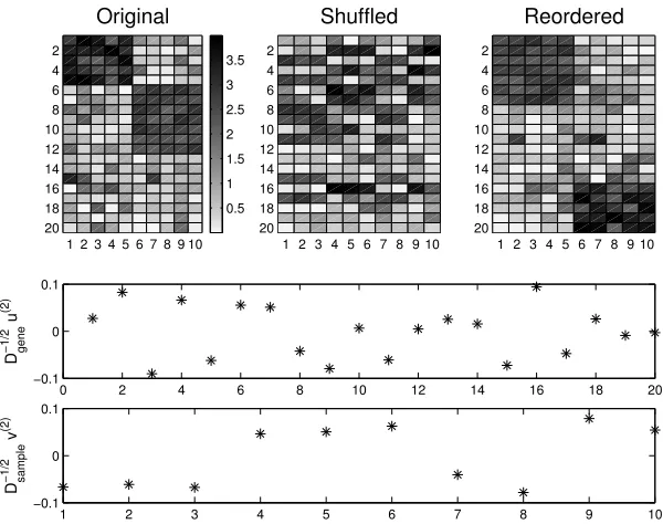
Fig. 5.1. Upper left: data matrix. Upper middle: shuffled. Upper right: reordered by spec-tral method. Lower pictures show components of the scaled second singular vectorsD−

1 2

geneu(2) _and

D−

1 2

samplev(2)ofD

−1 2 geneW D−

1 2 sample.

3 The quantityβsin (4.2), which is independent ofk, may be described as thetypical

connectivity for samples. It measures the weight associated with sample s

relative to the total amount of weight present.

4 Combining points 2 and 3, we see that in the iteration (4.1), the influence of sample

s on the new location of sample r depends on the difference between their actual and typical connectivities. If α[k]r,s > βs then sample r has a strong

connection with samplesand hence a positive weight is used in (4.1), which tends to bring the locations of samples r and s closer together at the next iteration. On the other hand ifα[k]r,s < βsthen samplerhas a weak connection

with sample sand hence a negative weight is used in (4.1), which tends to force the locations of samplesrands further apart at the next iteration.

Overall, this interpretation, which does not make use of advanced linear algebra concepts such as the SVD, shows that the spectral clustering approach may be viewed as a natural iteration that attempts to shuffle the location of the samples based on their relative connectedness. In addition to giving insight about the nature of the algorithm, this iterative viewpoint offers potential for customized versions, where existing knowledge about the existence of clusters could be built in at each iteration. This idea will be pursued in further work.

1 2 3 4 5 6 7 8 9 10 20

18 16 14 12 10 8 6 4 2

Shuffled

1 2 3 4 5 6 7 8 9 10 20

18 16 14 12 10 8 6 4 2

Reordered: 2nd sing. vecs

1 2 3 4 5 6 7 8 9 10 20

18 16 14 12 10 8 6 4 2

Reordered: 3rd sing. vecs 1 2 3 4 5 6 7 8 9 10

20 18 16 14 12 10 8 6 4 2

Original

0 1 2 3 4 5 6 7

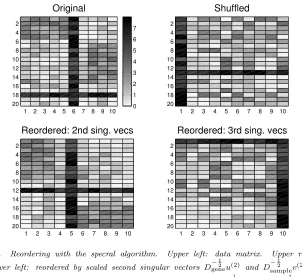
Fig. 5.2. Reordering with the specral algorithm. Upper left: data matrix. Upper right: shuffled. Lower left: reordered by scaled second singular vectors D−

1 2

geneu(2) _{and D}−12

samplev(2) of

D−

1 2 geneW D−

1 2

sample. Lower right: reordered by third scaled singular vectorsD

−1 2

geneu(3)_andD−12 samplev(3)

ofD− 1 2 geneW D−

1 2 sample.

generators according to

wij =

  

2 + 2rand, for 1≤i≤5,1≤j≤5,

2 +rand, for 6≤i≤12,6≤j≤10,

|randn_|, otherwise.

Here we follow MATLAB notation [10] so randand randndenote calls to Uniform ∈(0,1) and standard Normal generators, respectively. In summary,W has two blocks of relatively large entries that are clearly visible as darker pixels in the picture. For the purpose of visualization, the upper middle picture shows the same matrix with an arbitrary row and column shuffling. This is the matrix to which the algorithm is applied. (In practice, the algorithm is insensitive to permutations, but the middle picture represents the ‘unstructured’ format that would be generated in practice.) The middle and lower pictures in Figure 5.1 show the entries in the scaled second singular vectors of D−12

geneW D− 1 2

sample, that is D

−1 2

geneu(2) and D− 1 2

samplev(2), whereW denotes the

shuffled matrix. We see that the entries of D−12

geneu(2) fall into three bands and the

entries of D−12

samplev(2) fall into two bands. The component indices for the upper and

lower bands inD− 1 2

geneu(2)match the row indices for the two large blocks in the matrix.

Similarly, the component indices for the two bands in D− 1 2

samplev(2) match the column

indices for the two large blocks. To see this, the top right picture shows the matrix with rows and columns reordered according to the ordering of components inD−12

1 2 3 4 5 6 7 8 9 10 20

18 16 14 12 10 8 6 4 2

Shuffled

1 2 3 4 5 6 7 8 9 10 20

18 16 14 12 10 8 6 4 2

Reordered: 2nd sing. vecs

1 2 3 4 5 6 7 8 9 10 20

18 16 14 12 10 8 6 4 2

Reordered: 3rd sing. vecs 1 2 3 4 5 6 7 8 9 10

20 18 16 14 12 10 8 6 4 2

Original

0 1 2 3 4 5 6 7

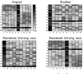
Fig. 5.3.As for Figure 5.2 except thatW is used instead ofD− 1 2 geneW D−

1 2

sample. Upper left: data

matrix. Upper right: shuffled. Lower left: reordered by second singular vectorsu(2) _andv(2) _ofW.

Lower right: reordered by third singular vectorsu(3) _andv(3)_{of W.}

andD−12

samplev(2). We see that the algorithm is able to recover the two blocks of large

entries.

In Figure 5.2, we repeat this exercise for a matrixW ∈R20×10 _{with entries}

wij =

          

1.5 + 2.5rand, for 1_≤i_≤5,1_≤j_≤5,

1.5 + 2.5rand, for 7_≤i_≤15,8_≤j_≤10,

4 + 4rand, fori= 18,1_≤j_≤10,

4 + 4rand, for 1≤i≤20, j= 6,

|randn|, otherwise.

Overall this matrix has two blocks of slightly larger than average entries, but is dom-inated by a large row (i = 18) and a large column (j = 6). This represents an unusually overexpressed gene and an unusually overexpressed sample. The top left picture shows the original matrix and the top right picture shows a row/column shuf-fled version, to which the algorithm was applied. The bottom left picture shows the reordered matrix, as described for Figure 5.1, and we see that the algorithm has suc-cessully located the two blocks, while placing the promiscuous row and column in the middle of the ordering. This agrees with the remarks made in sections 3 and 4. The lower right picture in Figure 5.2 shows the reordering produced by the scaled third singular vectors of D−12

geneW D− 1 2

sample, that is,D

−1 2

geneu(3) and D− 1 2

samplev(3). Here, the

In Figure 5.3 we perform the same experiment using the second and third singular vectors from the SVD ofW rather thanD−12

geneW D− 1 2

sample. Here, we see that reordering

with the second singular valuesu(2)_andv(2)_{serves only to isolate the outliers. Because}

there is no normalization across genes/samples, the algorithm is heavily influenced by the promiscuous values. However, the third singular vectors do pick out the remaining structure, namely the existence of the two significant blocks.

Overall, the tests here confirm that the SVD-based algorithm can successfully reveal the existence of clusters, and also support the earlier arguments that the normalization D−12

geneW D− 1 2

sample will tend to mitigate the influence of promiscuous

genes/samples.

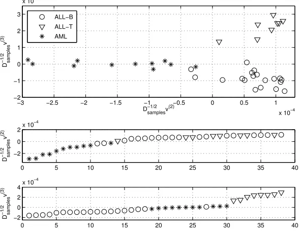
−3 −2.5 −2 −1.5 −1 −0.5 0 0.5 1 x 10−4 −2

−1 0 1 2 3

x 10−4

D−1/2 samplesv(2)

D

−1/2 samples

v

(3)

0 5 10 15 20 25 30 35 40 −2

0 2x 10

−4

D

−1/2 samples

v

(2)

0 5 10 15 20 25 30 35 40 −2

0 2 4x 10

−4

D

−1/2 samples

v

(3)

ALL−B ALL−T AML

Fig. 6.1. Leukemia: Upper: Scatter plot of the samples Lower pictures show samples ordered by the second and third singular vectors.

6. Microarray Data. To ilustrate the performance of the spectral algorithm proposed above we use acute leukemia data as published in [3]. The data set of bone marrow samples from 38 patients contains the expression intensities for 5000 genes. Twenty seven cases were diagnosed as acute lymphoblastic leukemia (ALL) and the other eleven as acute myeloid leukemia (AML). The distinction between ALL and AML, as well as the division of ALL into T and B cell subtypes, is well known. Several methods have been used to rediscover these differences [3], [5], [11], [13] and the leukemia data set has become a benchmark in the cancer classification community. The two lower pictures in Figure 6.1 show the reordering produced by the scaled second and third singular vectorsD−12

samplev(2)andD

−1 2

samplev(3). We see that the second

upper part of Figure 6.1 shows a plot of the second versus the third scaled singular vectors. Leukemias are here clustered into the three main biological classes.

7. Conclusion. We have given theoretical support for the use of the SVD by deriving a spectral clustering method from two alternative viewpoints. Both deriva-tions give insights into the performance of the method and suggest that it will be insensitive to the presence of outliers. We focused on the application of co-clustering microarray data sets and showed that there is a natural way to normalize expression levels across genes and samples. Results on a publicly available leukemia data set demonstrated how the algorithm can be used to characterize different types of cancer.

Acknowledgement. We thank Nick Higham for suggesting the short proof of Lemma 3.3. This work was funded by EPSRC grant GR/S62383/01. DJH is sup-ported by a Research Fellowship from the Royal Society of Edinburgh/Scottish Ex-ecutive Education and Lifelong Learning Department.

REFERENCES

[1] U. Alon, N. Barkai, D. A. Notterman, K. Gish, S. Ybarra, D. Mack and A. J. Levine, Broad patterns of gene expression revealed by clustering analysis of tumor and normal colon tissues probed by oligonucleotide arrays, PNAS, 96 (1999), pp. 67456750.

[2] A. Ben-Dor, L. Bruhn, N. Friedman, I. Nachman and U. WashingtonTissue classification with gene expression profiles, RECOMB Tokyo Japan, 2000.

[3] J. P. Brunet, P. Tamayo, T. R. Golub and J. P. Mesirov,Metagenes and molecular pattern discovery using matrix factorization, PNAS, 101 (2004), pp. 4164–4169.

[4] I. S. Dhillon, Co-clustering documents and words using bipartite spectral graph partition-ing, Proceedings of the Seventh ACM SIGKDD International Conference on Knowledge Discovery and Data Mining(KDD), August 26-29, 2001, San Francisco, California, USA [5] G. Getz, E. Levine and E. Domany,Coupled two-way clustering analysis of gene microarray

data, PNAS, 97 (2000), pp. 12079–12084.

[6] G. H. Golub and C. F. Van Loan, Matrix Computations, Third ed., The Johns Hopkins University Press, Baltimore, MD, 1996.

[7] T. R. Golub, D. K. Slonim, P. Tamayo, C. Huard, M. Gaasenbeek, J. P. Mesirov, H. Coller, M. L. Loh, J. R. Downing, M. A. Caliguri, C. D. Bloomfield and E. S. Lander,Molecular classification of cancer: class discovery and class prediction by gene expression monitoring, Science, 286 (1999), pp. 531–537.

[8] P. Grindrod and M. Kibble,Review of uses of network and graph theory concepts within proteomics, Expert Rev. 1 (2004), pp. 229–238

[9] D. J. Higham and M. Kibble,A unified view of spectral clustering, University of Strathclyde Mathematics Research Report 02 (2004).

[10] D. J. Higham and N. J. Higham,MATLAB Guide, SIAM, 2000.

[11] Y. Kluger, R. Basri, J. T. Chang and M. Gerstein,Spectral biclustering of microarray data: coclustering genes and conditions, Genome Research, 13 (2003), pp. 703–716. [12] S. Rogers, M. Girolami, C. Campbell and R. Breitling,The latent process decomposition

of cDNA microarray datasets, IEEE/ACM Transactions on Computational Biology and Bioinformatics, to appear.

[13] J. Wang, T. H. Bo, I. Jonassen,O. Myklebost and E. Hovig, Tumor classification and marker gene prediction by feature selection and fuzzy c-means clustering using microarray data., BMC Bioinformatics, 4 (2003), 60.