Depth spreading through empty space induced by sparse disparity cues

City, University of London Institutional Repository

Citation

:

This is the accepted version of the paper.

This version of the publication may differ from the final published

version.

Permanent repository link:

Link to published version

:

Copyright and reuse:

City Research Online aims to make research

outputs of City, University of London available to a wider audience.

Copyright and Moral Rights remain with the author(s) and/or copyright

holders. URLs from City Research Online may be freely distributed and

linked to.

City Research Online: http://openaccess.city.ac.uk/ [email protected]

Depth Spreading through Empty Space Induced by Sparse Disparity Cues

Xintong Li1

, Abigail E. Huang1

, Eric L. Altschuler1

, Christopher W. Tyler2

1

New Jersey Medical School

Abstract

Introduction

The primary goal of visual encoding is to determine the nature and motion of the objects in the

surrounding environment. In order to plan and coordinate actions, we need a functional

representation of the three-dimensional (3D) scene layout and of the spatial and depth

configuration of the objects within it. The visual information provided to each eye is, however,

two-dimensional (2D), and the 2D configurations of objects in the visual array have an entirely

different metric structure from that of the spatial configuration of the visual cues that convey the

presence of objects to the brain, or to artificial sensing systems that share none of the physical

properties constituting the objects. In general, the visual cues may change in luminance or color,

or they may be disrupted by reflections or occlusion by intervening objects. The particular cues

such as edge structure, binocular disparity, color, shading, texture, and motion vector fields may

carry discordant information about different aspects of an object. Importantly, many of these

cues may be sparse, with missing information about the object structure across occlusions or

gaps where there are no edge or texture cues to carry information about the object shape.

Thus, a primary requirement of neural or computational representations of the shape of

objects is the reconstruction of the 3D configuration and filling-in of its depth surfaces across

regions of missing or discrepant information in the local visual cues. Computational approaches

to the issue of the structure of objects tend to take either low-level or high-level approaches to

the problem. Low-level approaches begin with local feature recognition and attempt to build up

the object representation by hierarchical convergence, using primarily feedforward logic with

some recurrent feedback tuning of the results (e.g., Marr, 1982; Grossberg, Kuhlman &

Mingolla, 2007). High-level, or Bayesian, approaches begin with the vocabulary of likely object

structures and look for evidence in the visual array as to which object might be there (e.g., Huang

& Russell, 1998; Rue & Hurn, 1999; Moghaddam, 2001; Stormont, 2007). Both approaches

work well for objects with a stable 2D structure (as in a typical laboratory set-up), but are easily

confused when viewing a complex 3D scene (such as a hardware store). It is therefore of critical

importance in full-fledged visual representation to provide a completed reconstruction of the 3D

Surfaces as a Mid-Level Invariant in Visual Encoding

Rather than relying on the object templates typical of cognitive investigations, a more

fruitful approach to the issue of 3D object structure is to focus the analysis on mid-level invariants to the object structure, such as surfaces, symmetry, rigidity, texture invariants or

surface reflectance properties. Each of these cues is invariant under transformations of 3D pose,

viewpoint, illumination level, haze contrast, and other variations of environmental conditions.

Various computational analyses have incorporated such invariants in their object-recognition

schemes, but a neglected aspect of mid-level vision is the 3D surface structure that is an

inescapable property of objects in the world.

Surfaces are a key property of our interaction with objects in the world. It is very unusual

to experience objects, either tactilely or visually, except through their surfaces. Even transparent

objects are experienced through their surfaces, with the material between the surfaces being

invisible by virtue of the transparency. Only translucent objects are experienced in an interior

manner, as the light passes through them to illuminate the density of the material. Developing a

means of representing the proliferation of surfaces before us is, therefore, a key stage in the

processing of objects.

The various 3D surface cues such as luminance shading, linear perspective, aspect ratio

of square objects, and texture gradient can each specify the slant of a planar surface. Zimmerman,

Legge & Cavanagh (1995), for example, performed experiments to measure the accuracy of

surface slant from judgments of the relative lengths of a pair of orthogonal lines embedded in

one surface of a full visual scene. Slant judgments were accurate to within 3 deg for all three cue

types, with no evidence of the recession to the frontal plane expected if the pictorial surface was

contaminating the estimations. Depth estimates of disconnected surfaces were, however, strongly

compressed. Such results emphasize the key role of 3D surface reconstruction in human depth

estimation. .  

Surface Representation through the Attentional Shroud

A more vivid representation of the depth reconstruction process is to envisage it as an

‘attentional shroud’ (Tyler & Kontsevich, 1995; Tyler, 2005; Huang et al., 2012), wrapping the

dense locus of activated disparity detectors as a cloth wraps a structured object. The concept of

the attentional shroud can also be the thought of as a mechanism that acts like a soap film in

information. To probe the nature of object processing by different cues, we may measure the

localization of objects defined by multiple visual modalities (such as luminance and disparity).

Likova & Tyler (2003) addressed the unitary depth map hypothesis of object localization

by using a sparsely sampled image of a Gaussian bulge. The sparse sampling dramatically

degraded localization accuracy based on luminance cues, but caused no degradation when based

on binocular disparity cues. This dramatic difference suggests that depth surface reconstruction

is the key process in the accuracy of the localization process. Furthermore, when depth was

nulled by opposing the luminance and disparity cues, localizing the ‘object’ (the Gaussian bulge)

became impossible. Only an interpolation mechanism operating at the level of generic depth representation can account for the data. Evidently, the full specification of objects in general

requires extensive interpolation to take place. The dominance of a depth representation in the

performance of such tasks indicates that the depth information is not just an overlay to the 2D

sketch of the positional information. Instead, a full 3D depth reconstruction of the surfaces in the

scene must be completed by the human visual system before the position of the object is known.

Rationale

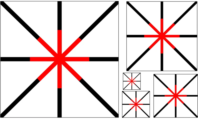
To address the question of depth reconstruction in the sparse cue situation, we designed a depth image that is a 3D version of the neon color spreading effect (Figure 1), in which the empty wedge regions between the spokes appear to take on a fainter version of the color of the central segments of the spokes (Varin, 1971; van Tuijl, 1975; Bressan et al., 2003). It is generally understood that the colored region has the form of a circular disk (e.g., Gove et al., 2005), although the sharpness of the edges does not appear to have been quantified and our close observation suggests that the edge region is not well defined and cannot be definitely specified as having the sharp edge of a uniform disk.

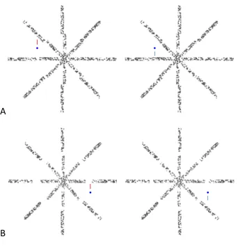
Figure 2. The Depth Spreading Effect, a stereoscopic depth version of the Neon Color Spreading Effect. Free fusion across a pair of these images will reveal a pair of stereoscopic images, one with near and the other with far

disparity in the central region of spokes, which appears to complete across the white spaces to form a raised or

recessed disk.

implying a 100% strength of the depth filling-in effect, in contrast to the much weaker filling-in of the neon color spreading effect.

Depth spreading through empty space was reported by Julesz (1971, Figure 7.7.1), in the form of a white stripe through his classic random-dot stereogram of a depth square. He described the perceived depth as forming a “crisp contour”, and showed that a more complex type of interpolation in the form of a white stripe through a random-dot stereogram of a diamond shape Julesz (1971, Figure 7.7.2) did not give a clear interpolated border. He did not, however, quantify the sharpness of the border, and did not assess the form of a curved border interpolation. Gove et al. (2005) implemented a computational model of the neon color spreading through the LAMINART model of cortical interactions (Grossberg, 1999) that generated a linear contour interpolation. Presumably a more elaborated process would be needed to generate a fully circular completion boundary, either one that was anisotropic, with extended smoothing along the contour while allowing propagation of the sharp boundary across the contour, or one that incorporates relaxation to simple higher-order figures such as circles.

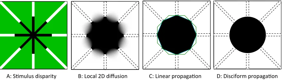
These possibilities for the process involved in the completion of the disk, in either the color or depth version of the filling-in, can be formalized into the four hypotheses depicted in Figure 3:

1. Low-level local depth propagation: local diffusion hypothesis that the filling-in fades gradually towards the edge in a form predicted by a local 2D diffusion function to form depth gradients in the wedge regions (Figure 3B). (Details of the 2D diffusion hypothesis are provided in Methods.)

2. Mid-level depth-contour propagation: A. Linear depth-contour extrapolation hypothesis that the filling-in propagates the sharp-edged character of the defined disparity terminator edges linearly across the undefined region, such that the shape of the filled-in region extends along the orientation of the terminators to take an octagonal form (Figure 3C, green contour). B. Linear depth-contour interpolation hypothesis that the filling-in propagates the sharp-edged character of the defined disparity terminations linearly across the undefined region, such that the shape of the filled in region takes a truncated octagonal form (Figure 3C, black boundary).

filled in uniformly up to the edge and falling immediately to the surround level beyond the edge (Figure 3D).

!A:!S%mulus!disparity !B:!Local!2D!diffusion !C:!Linear!propaga%on !D:!Disciform!propaga%on!

Figure 3. Depiction of three forms of depth surface interpolation. A: stimulus disparity arrangement (black to white: far to near

disparities, green: undefined). B: depth interpolation by diffusion from the spokes, forming depth gradients in the wedge regions. (Black to white: far to near perceived depth, dashed lines: region of defined disparity). C: Two forms of depth propagation with straight contours in forming a sharp-edged octagon between the spokes. The green outline depicts linear extrapolation of the depth contours in the spokes; the cyan outline around the black octagon indicates linear interpolation between the endpoints of the depth contours D: depth propagation along curved contours in the form of a sharp-edged disk.

This study is designed to measure the form of the depth profile in the interpolation region in order to gain insight into the neural mechanisms involved in the interpolation process.

Methods

Subjects and Experimental Setup

Four naïve subjects, all with normal or corrected-to-normal vision and able to free-fuse the adjacent pair of (non-anaglyphic) binocular stimuli comfortably, each performed binocular observations at a viewing distance of 86 cm of the stereoscopic patterns presented on a pixelated computer screen with a horizontal resolution of 1024 pixels. The study was approved by the UMDNJ IRB, and all subjects gave written informed consent.

Stimuli

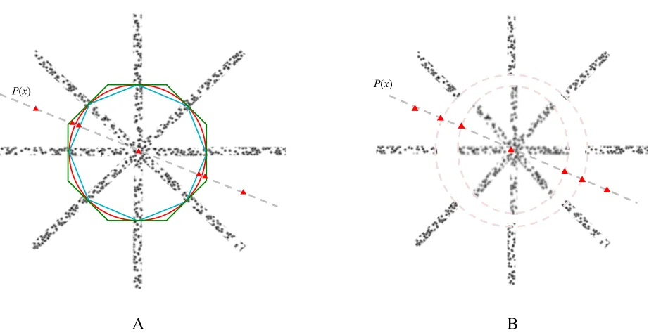
length and composition, with a disparity offset from that of the outer spokes. In the frontoparallel set, these inner spokes were given a uniform disparity of -23 arcmin when viewed binocularly, with the random dots forming a continuous pattern through the region of the disparity edges within the spokes. In the horizontally slanted configuration, the spokes were arranged to lie in a slanted plane with the left edge at a disparity of -28 arcmin and the right edge at a disparity of +11 arcmin when viewed binocularly. To control for any interference from the monocular vernier-type shifts present in the uniform disparity condition (Figure 2), the slanted condition also included a gap between the inner and outer spokes (Figure 4B).

!!

1

P(x) P(x)

                         A                        B

Figure 4. A. Diagram of non-slanted test image with red triangles indicating tested locations and blue, green, and red lines

Figure 5. A.Example of the non-slanted stimulus configuration that subjects were asked to free-fuse to test the sharpness of the

depth boundaries. Blue test dots are set at the upper radial position just outside the circular boundary of the inner disc, the red fiducial line is aligned with the blue dots in the right eye, and the cyan line in the left eye, to form a Nonius pair. B. Example of the slanted stimulus configuration, with the blue test dot and Nonius lines set at the lower radial position just outside the circular boundary.

Procedures

stepped the blue dot pair through the 9 available disparity levels in sequence to find a perceived depth match, with the capability of going back and forth along the sequence to refine their choice when they were close to their perceived match. Both sets of frontoparallel and horizontally slanted depth structures were run for each of two experiments to evaluate the perceived depth in the intervening white spaces and the sharpness of depth boundaries.

Perceived depth of white space

Perceived depth of the white space interpolated from the inducing spokes was first quantified to test the observation that depth did spread into the empty space of the gaps between spokes. Subjects selected the stimulus in which the disparity of the blue dot appeared to lie at a depth that matched their perceived depth of that space (Figure 4). This process was repeated for each of seven positions along the radial line per set of frontoparallel and horizontally slanted inner disks: in the empty space between the outer spokes, depth boundary of the outer spokes, depth boundary of the inner spokes, middle of the illusory depth structure, and three corresponding positions on the opposite side of the structure (Figure 4).

Radial position was the distance in pixels from the outer radial boundary of the outer spokes to the point of interest. This was measured as viewing angle in arcmin by multiplying the

angle in radians by   . Disparity was measured in pixels shift, as follows:

Equation 1. Disparity as measured by pixels in arcmin.

Predictions

hypothesis predicts that a sharp depth contour in the empty white space is at the same radial distance as the disparity edge in the spokes (i.e., 0.5). (Only the disciform hypothesis was evaluated for the slanted configuration because the gaps between the inner and outer spokes made the others difficult to implement.) Radial distance from the center was specified in arcmin (Figure 6C). Depth value outputs with the same range were rescaled to the respective actual disparities of the outer boundary of the inner illusory disk and the inner boundary of the outer spokes. !! !! !!!! !! !! !! !! !!

0 1 2

!! !! !! !! !! !! !!

A B C

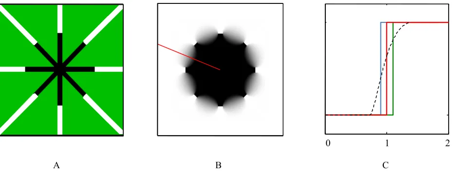
Figure 6. Perceived depth predictions of the four hypotheses. A. Illustration of the disparity configuration of the stimulus of

Figure 4A, with white and black designating the two disparities and green designating indeterminate white regions. B. Surface interpolation in radial distance (θ = π/8) calculated using MATLAB’s TriScatteredInterp function. The red line in B indicates the radial position of the depth of the interpolated surface in (C). C. Hypothetical perceived depth functions. The red line in C portrays the hypothesis of a sharp border on a curved (disciform) contour at the same radial distance as the disparity edges, in contrast to the linear extrapolation of the disparity contours (green line), linear interpolation of the sharp border between the disparity contour endpoints (cyan line) and the surface interpolation hypothesis of panel B (dashed line).

Sharpness of depth boundaries

empty space: once for the circular depth boundary of the outer spokes, once for the boundary of the inner spokes, and finally once each at the two corresponding positions on the opposite half of the structure. Pixel distances were converted into arcmin for further statistical analysis using the same conversion factor as in Equation 1. The distance from the center of the inner spokes to the midpoint of any edge of an interpolated octagonal depth boundary was determined as follows, where r is the length of any inner spoke and the radius of an interpolated circular boundary:

  .

Equation 2. Distance from center of inner spokes to midpoint of the edge of interpolated octagonal depth boundary, with r being

the radius of interpolated circular boundary.

Thus, the octagonal extrapolation predicts a distance ratio of 1.082 times that of the circular interpolation while the octagonal interpolation predicts a distance ratio of 0.924.

Results

Figure 7. Graphical representation of the results and predictions for each set of frontoparallel (A) and horizontally slanted (B) depth structures. shows our actual results, depicts the surface interpolation, and illustrates the depth interpolation; n = 4.

Table IA. Perceived Depth Predictions and Results for the Unslanted Display

Radial position

Depth predictions

Actual

results SD Linear interpolation Linear extrapolation Disciform hypothesis Local depth propagation

-270 0* 0* 0 0* -2.1 0.5

-155 0* -23* 0 -5.6* -1.6 2

-150 0* -23* -23 -7* -22.6 0.7

0 -23* -23* -23 -23* -22.3 0.5

150 0* -23* -23 -7* -22.3 0.5

155 0* -23* 0 -5.6* -0.5 0.8

270 0* 0* 0 0* -0.5 0.8

Table IB. Perceived Depth Predictions and Results for the Slanted Display

Radial position

Disciform hypothesis

Actual

results SD

-270 0 0.5 1.9

-160 0 -0.5 1.2

-140 -28 -26.5 1.6

0 -7 -7.4 0.5

140 11 11.1 1.9

160 0 -1.1 1.3

Table 1. Depth predictions for several hypothetical forms of depth spreading compared with results from naïve subjects (n = 4) with standard deviation (SD) at each of 7 radial positions (bolded) for the frontoparallel (A) and horizontally slanted (B) depth structures at radial positions designed to discriminate among the hypotheses of Figure 6. All measurements in arcmin of the visual angle of subtense. Asterisks in A (*) indicate significant differences (p < 0.05, corrected for multiple applications across the tables, n = 4) between observed and predicted depth values for a particular model (see Figure 7A). Values in B were only evaluated for the disciform hypothesis, for which the data showed no significant differences from the predicted depths (see Figure 7B).

Sharpness of depth boundaries

From the data, Gaussian plots depict the mean at the inner depth boundaries to quantify sharpness and boundary position relative to the three hypotheses (Figure 7). The data from boundary sharpness are consistent with the prediction of a circular and not either of the octagonal depth structures. Gaussian distributions of lateral shift data for the frontoparallel set indicate that the location of the border is remarkably precise (Figure 7), with σ of the order of 5 arcmin, or only about 2% of the radius of the disk. At a criterion of p < 0.05, the disciform hypothesis is the only one that is not significantly different from observed values of depth, while being significantly different from the two locations predicted by the other two hypotheses (see Figure 7).

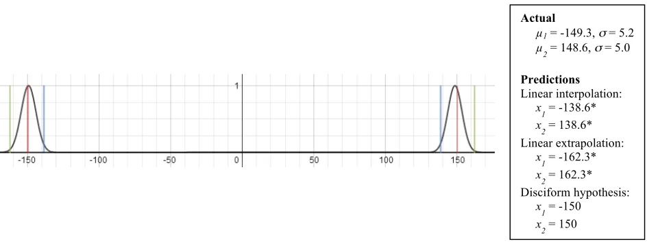
Figure 8. Results of the position estimation of the perceived border for the frontoparallel disc. Gaussian curve represents the

mean and standard deviations (σ) of the results. Vertical bars represent the predicted locations of the interpolated (blue),

extrapolated (green), and circular (red) hypotheses as to the position of the perceived depth border. Asterisks (*) indicate predicted values for which the actual depth differed significantly (p < 0.05, n = 4).

Discussion

Actual

µ1 = -149.3, σ= 5.2 µ₂ = 148.6, σ= 5.0

Predictions

Linear interpolation:

x₁ = -138.6*

x₂ = 138.6* Linear extrapolation:

x₁ = -162.3*

x₂ = 162.3* Disciform hypothesis:

x₁ = -150

This study had two main outcomes. First is that there is perceptual completion of the disparity border specified in the spokes across the empty white space between the spokes, forming a perceived depth border as sharp as could be measured by our probe technique. This is an anisotropic form of diffusion, in that the border is propagated lengthwise between the spokes rather than spreading out isotropically from the points where the disparity information stops. We formalized the isotropic diffusion concept as a local diffusion process of the 3D surface information provided by the disparity in the spoke regions, predicting the 2D surface function depicted in Figure 3B and graphed as a 1D function through the line halfway between the spokes in Figures 4 and 6B. This diffusive form of interpolation is strongly repudiated by the quantitative results, which show that the perceived border is much sharper than the isotropic 2D diffusion prediction, requiring some form of anisotropic diffusion in which the border information is propagated only along a 1D linear extension of its length and not in any other directions.

This raises the issue of the second outcome, which shows what form of line the 1D propagation takes. The two forms depicted in Figure 3C are incompatible with the results in Figure 7, which shows that the location of the sharp depth border is conforms only to the fourth hypothesis of anisotropic curvilinear extrapolation of the disparity edges to form a homogeneous flat disk in depth. Whereas the isotropic 2D propagation and the anisotropic 1D propagation hypotheses are compatible with local processes, the anisotropic disciform propagation seems to be compatible only with a global process that conforms the interpolated depth contours into a figural Gestalt with global simplicity. Admittedly, a disk shape is a very familiar form of global simplicity, but it is nevertheless one that has to be applied to the perceived depth structure, which is itself a higher-order construct relative to the local luminance edges that are considered the usual constituents of form processing. The disciform outcome of the interpolation process is therefore a substantial challenge to an understanding of the underlying perceptual mechanisms in terms of local neural processes.

roundish recess generated by a proto-interpolation process might be guided toward the form of a disk because of its figural simplicity.

The other possible mechanism is the Bayesian prior, which says that, regardless of figural properties, the interpolation is governed by the probability of having encountered recesses of various shapes in the past. The highest probability shapes then tend to govern the shape that the present recess is perceived to have. It should be noted that the Bayesian hypothesis is entangled with the transformational invariance hypothesis in two respects. One is that the recesses encountered in the past may themselves be biased toward a rotationally invariant sample because many of them may have been made by a rotationally invariant tool such as a drill (or a molding derived from such a tool). In this respect, our modern visual systems brought up in a ‘carpentered’ artificial environment might be very different from those brought up in a primitive cave environment, in which accurately disciform recesses would be extremely rare. The other is that, conversely, the average probability function for recess shapes would tend toward rotational invariance even though the individual examples encountered might not themselves have been circular, simply by regression toward the mean. On this argument, the Bayesian prior might tend toward simplicity principles in the average even if they were not manifested in individual examples. In general, then, it is likely to be difficult to disentangle the mechanism enforcing the simplicity interpretation unless studies are done to specifically distort the near-term Bayesian prior and determine its degree of applicability in particular cases.

Acknowledgments

References

Bach M. (2002) Neon color spreading. 100 Visual Phenomena & Optical Illusions Website (http://michaelbach.de/ot/col_neon/index.html).

Bressan P, Mingolla E, Spillmann L, Watanabe T (1997) Neon color spreading: a review. Perception 26: 1353–1366.

Huang PC, Chen CC, Tyler CW (2012) Collinear facilitation over space and depth. J Vision 21;12(2). pii: 20. doi: 10.1167/12.2.20.

Grossberg S (1999) How does the visual cortex work? Learning, attention and grouping by the laminar circuits of the visual cortex. Spatial Vision 12:163-186.

Grossberg S, Kuhlmann L, Mingolla E (2007) A neural model of 3D shape-from-texture: multiple-scale filtering, boundary grouping, and surface filling-in. Vision Res.47:634-72

Huang T, Russell S (1998) Object identification: A Bayesian analysis with application to surveillance. Artificial Intell. 103:1-17.

Julesz B (1971) Foundations of Cyclopean Vision. University of Chicago Press: Chicago IL.

Likova LT, Tyler CW (2003) Peak localization of sparsely sampled luminance patterns is based on interpolated 3D object representations. Vision Res.43: 2649– 2657.

Marr D (1982) Vision: a Computational Investigation into the Human Representation and Processing of Visual Information. W.H. Freeman and Company, NY.

Moghaddam B (2001) Principal manifolds and probabilistic subspaces for visual recognition. IEEE Trans. Pattern Anal. Machine Intell 24:780-788

Norman JF, Todd JT (1998). Stereoscopic discrimination of interval and ordinal depth relations on smooth surfaces and in empty space. Perception, 27:257– 272.

Rue H, Hurn MA (1999) Bayesian object identification. Biometrika 86:649-660

Stormont DP (2007) An Online Bayesian Classifier for Object Identification. IEEE International Workshop on Safety, Security and Rescue Robotics, 2007, 1-5.

Tyler CW (2005) Spatial form as inherently three-dimensional. In Seeing Spatial Form, Jenkin MRM, Harris LR (Eds). Oxford University Press: Oxford, Ch. 6.

Tyler CW, Kontsevich LL (1995) Mechanisms of stereoscopic processing: stereoattention and surface perception in depth reconstruction. Perception, 24: 127–153.

Varin D (1971) Fenomeni di contrasto e diffusione cromatica nell organizzazione spaziale del campo

percettivo. Rivista di Psicologia 65:101-128.