Comparison of four digital halftone screen (dither) patterns using quantitative analysis of the binary image microstructure

Rochester Institute of Technology

RIT Scholar Works

Theses

Thesis/Dissertation Collections

3-1-1989

Comparison of four digital halftone screen (dither)

patterns using quantitative analysis of the binary

image microstructure

Jacquelyn S. Ellinwood

Follow this and additional works at:

http://scholarworks.rit.edu/theses

This Thesis is brought to you for free and open access by the Thesis/Dissertation Collections at RIT Scholar Works. It has been accepted for inclusion in Theses by an authorized administrator of RIT Scholar Works. For more information, please [email protected].

Recommended Citation

COMPARISON OF FOUR DIGITAL HALFTONE SCREEN (DITHER) PATIERNS USING QUANTITATIVE ANALYSES OF THE

BINARY IMAGE MICROSTRUCTURE

by

Jacquelyn S. Ellinwood

A thesis submitted in partial fulfillment of the requirements for the degree of

Master of Science in the Center for Imaging Science in the College of Graphic Arts and Photography of the

Rochester Institute of Technology

March 1989

Signature of Author J_a_c--=qu=----e_l..=y_n_S_._E_l_l_~_·n_w_o_o_d _

Accepted by N_arn_e_ _I_l_l_e..=g_i_b_l_e _

COli.EGE OF GRAPHIC ARTS AND PHOTOGRAPHY ROCHESTER INSTITUTE OF TECHNOLOGY

ROCHESTER, NEW YORK

CERTIFICATE OF APPROVAL

M.S. DEGREE THESIS

The M.S. Degree Thesis of Jacquelyn S. Ellinwood has been examined and approved

by the thesis committee as satisfactory for the thesis requirement for the

Master of Science degree

Mr. Peter Engeldrum, Thesis Advisor

Dr. Roger Easton

Dr. Rodney Shaw

htvr.t

jJ

ry;(

j

7

If

THESIS RELEASE PERMISSION FORM

ROCHESTER INSTITUTE OFTECHNOLOGY COLl.EGE OF GRAPHIC ARTS ANDPHOTOGRAPHY

Title of Thesis: Comparison of Four Digital HalftoneScreen<Dither) Patterns Using Quantitative AnalYsis of the Binary Image Microstructure

I, Jacquelyn Ellinwood, hereby grant permission to the Wallace Memorial Ubrary of R.I.T. to reproduce my thesis in whole or in part. Any reproduction will not be for commercial use or profit.

Signature: _ _..;;;,J.=a..;;;,c....:ilquo..=e..;;;;l.-.y...n:...=E..;;;;l..;;;;l..;;;;i...n ...w...:.o...:.o...:.d;..._ _

COMPARISON O F FOUR DIGITAL HALFTONE S C R E E N (DITHER) PATTERNS USING QUANTITATIVE ANALYSES OF THE

BINARY IMAGE MICROSTRUCTURE

by

Jacquelyn S . Ellinwood

Submitted to the Center for Imaging Science in partial fulfillment of the requirements

for the Master of Science Degree at the Rochester Institute of Technology

ABSTRACT

The ordered-dither halftoning technique which reproduces continuous tones with spatially encoded binary imaging elements uses the digital halftone screen. The effect at the microstructural level of four screens on tone reproduction, spatial signal reproduction, and quantization noise is evaluated by measuring the tone reproduction curve (TRC), the two-dimensional Fourier transform of a constant density patch, the degree of harmonic distortion (THD), the system Modulation Transfer Function (MTF), and the Wiener Spectrum (WS) produced by each screen. The applicablity of these five conventional image evaluation metrics on binary output is also evaluated. Spatial averaging is done to convert the binary output to a more linear form.

The T R C s were found to be identical with a full output average reflectance range and a contrast of 1.0/255.0. The curves were step-wise linear, displaying 65 reproducible average reflectance levels. Fourier analysis of the binary structure showed that aliasing was likely to occur with the

Diamond Dot and Bryngdahl screens, while aliasing from the Bayer and Allebach screens was unlikely. The THD plots showed that the Diamond Dot screen produced the highest degree of non-linearity, followed by Bryngdahl. The Bayer and Allebach screens produced the lowest THD. The line edge derivative approach to determining MTF did not yield useful MTF results for the halftoned forms. The Weiner spectrum for the Diamond Dot and

ACKNOWLEDGEMENTS

Successful completion of this thesis owes recognition to support from many sources. Valuable and timely assitance and advice was particularly appreciated from the following:

Peter Engeldrum, currently of Imcotek Inc., who has acted as thesis advisor as well as mentor. His help in planning, organizing, and understanding the work has been invaluable. Pete's knowledge of the subject, enthusiasm, and willingness to help has been unrivaled.

Rodney Shaw and Roger Easton of the Center for Imaging Science (CIS) at RIT who have acted on the thesis committee. A special thanks is given for

Rodney's technical insights and for Roger's assistance in the writing of a clear and concise thesis.

Robert Fiete and Jennifer Wideman, two Eastman Kodak colleagues who offered invaluable peer-level input on the depth and clarity of the work and presentation. Their excitement about the results was contagious.

Paul Flavin and Chia-Chin Liu, RIT colleagues who provided digital imagery used for realizations, and supplied and supported computer programs that generated the halftone realizations. Their cooperation saved numerous hours of work.

Thomas Ellinwood, my husband, and Bernard and Carol Whaley, my parents, who have provided continued support throughout my education. Tom has been very supportive of my academic decisions and has never asked that boundaries be set on the time and energy that I spent in pursuit of my degrees. Mom and Dad offered financial support for over half of my education, supplied a

I. Introduction 1

1.0 Traditional Halftoning vs. Digital Halftoning 1

1.1 Traditional Halftoning 3

1.2 Digital Halftoning • 7

2.0 Digital Halftone Screen Patterns 11

2.1 Diamond Dot Screen 12

2.2 Bryngdahl-type Screen 13

2.3 Bayer-type Screen 15

2.4 Allebach-type Screen . - . 1 6

3.0 Objective •• •• 19

II. Evaluation Methods • 20

1.0 Tone Reproduction Analysis • 22

2.0 Tone Uniformity Analysis (Aliasing) 26

3.0 Harmonic Distortion Analysis 27

3.1 Total Harmonic Distortion 28

3.2 Fisher's Test of Harmonic Significance 30

4.0 System Modulation Transfer Function Analysis 31

III. Experimental Parameters 37

1.0 Halftone Screens 39

1.1 Halftone Cell Size 39

1.2 Halftone Cell Scale 41

2.0 Halftone Threshold Values 41

3.0 Test Patterns 42

IV. Results 50

1.0 Tone Reproduction Analysis 56

2.0 Tone Uniformity Analysis (Aliasing) 58

3.0 Harmonic Distortion Analysis 60

4.0 System Modulation Transfer Function Analysis ..62

5.0 Quantization Noise Analysis 66

V. Discussion 69

1.0 Tone Reproduction Analysis • 69

2.0 Tone Uniformity Analysis (Aliasing) 70

3.0 Harmonic Distortion Analysis • 73

4.0 System Modulation Transfer Function Analysis 75

5.0 Quantization Noise Analysis 77

1.0 Traditional Halftoning vs. Digital Halftoning

A halftone is a reproduction of a continuous-tone image that uses binary output

to create the perception of intermediate tones. The illusion of different density levels in

a halftone is due to the observer's vision; the imaging elements are made so small that

the eye is unable to resolve each individual element. An intermediate density level is

perceived when the visual system, acting as a spatial integrator, averages the imaging

elements and substrate density together over some area. The area covered by the imaging

element relative to the aperture area defines fractional area coverage (equation 1).

Average reflectance and average density are functions of fractional area coverage

(equations 2 and 3).

^ aperture area = A

area covered by imaging element = a

f = a/A (1)

f = fractional area covered by dark imaging element A = aperture area

a = area within A covered by imaging element

R = [R(p)x(1-f)] + [R(i)xf] (2)

R = average reflectance

R(p) = reflectance of paper or substrate R(i) = reflectance of imaging element

D = -log [R]

= -log([R(p)x(1-f)] + [R(i)xf]) (3)

D = average density

Henry Fox Talbot, a British pioneer in photography, made use of the visual

perception of changing fractional area coverage when he invented the traditional halftone

process in 18521. By the late 1800s halftoning had become a popular method of

reproduction in the printing industry2. When computers became popular in the 1970s

and 1980s, digital image reproduction methods replaced a large part of the traditional

halftoning processes. Numerous digital halftoning algorithms were developed to

maximize aesthetic qualities such as tone, dynamic range, and resolution of the output

image. One of the most popular methods is the ordered-dither. With this method a set of

non-image-related values contained in a halftone screen is added to a digitized scene. The

sum is thresholded and assigned an 'on' or 'off value at each location. The screen cell

Lippel and Kurland5, and o t h e r s6'7-8-9'1 0'1 1 have published articles on particular

halftone screen patterns and their effects, while Stoeffel and M o r e l a n d1 2, and Jarvice,

et. a / .1 3 have published comprehensive surveys on the subject. In addition, A l l e b a c h1 4,

Floyd and S t e i n b e r g1 5, and others16,17,18,19,20,21 n a ve reported algorithms other

than ordered-dither.

While the literature contains both subjective and objective analyses on effects of various digital halftone screens, a quantitative analysis using the methods outlined in

Section II does not exist. Since the halftone screen pattern strongly influences final image characteristics, it is important to understand the effects of a given pattern on an image. First, though, an understanding of the digital halftoning process and how it relates to traditional halftoning is important.

1.1 Traditional Halftoning

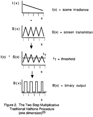
B r y n g d a h l2 2 describes the traditional halftoning process in mathematical terms

l ( x )

I I

l(x) = scene irradiance

S ( x )

MM

l(x) * S(x)

I I I I I

A A M

i i i

B ( x )

I I I

S(x) = screen transmittance

I j = threshold

B(x) = binary output

Figure 2. The Two Step Multiplicative Traditional Halftone Procedure

(one dimension)2 3

Because transmittances multiply the traditional photographic process is

considered multiplicative. For the case above, the original scene with irradiance l(x) is

photographed through a halftone screen with transmittance S(x). The screen function

S(x) introduces a non-image related light distribution to the exposed image. In

traditional contact screen halftoning, a physical halftone screen is placed in contact with

the film, between the original scene and the film. The older cross-line screen used in a

The lines are etched or scratched into clear plastic or glass. This screen is placed at a

distance from the film, thus casting a defocussed image on the film. An example of a

traditional cross line halftone screen that is commonly used in a graphic arts camera is

shown in figure 3.

^ 1 m m w

Figure 3. Example of a Traditional Cross Line Halftone Screen

The product of the scene irradiance and the screen transmittance is subjected to

an irradiance threshold, \j, by projecting the scene onto a high-contrast recording film.

Density

Irradiance

T

Figure 4. Thresholding Effect

Characteristic Curve of High Contrast Recording Film

After processing, dark elements occur in the final image, B(x), when

l(x) x S(x) > lT

The final image, B(x), is a matrix of imaging elements of varying size placed on paper

or some other receiver substrate. In figure 5, the traditional halftone binary structure

is shown.

These imaging elements vary the fractional area coverage by a change in size.

Since the fractional area coverage can assume any value between 0.0 and 1.0, an infinite

number of density levels in the final image between minimum and maximum density is

possible.

1.2 Digital Halftoning

As in traditional multiplicative halftoning, digital halftoning converts a

"continuous tone" input image into binary output. The input image is quantized to digital

values, called pixels or pels, that represent the gray level in the original image.

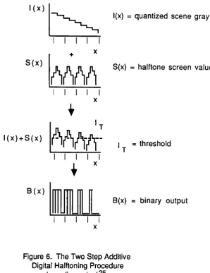
B r y n g d a h l2 4 describes the digital halftoning process as additive (figure 6). A computer

is capable of using the multiplicative or the additive approach. In digital halftoning,

though, the additive scheme is usually used because add instructions are faster than

l ( x )

l(x) = quantized scene gray level

S ( x )

I I I I

S(x) = halftone screen value

I I I

l ( x ) + S ( x )

I I I I I

I

B ( x )

= threshold

B(x) = binary output

Figure 6. The Two Step Additive Digital Halftoning Procedure

(one dimension)2 5

For the case in Figure 6, the quantized scene gray level l(x) is added to the halftone

screen value, S(x). The halftone screen is known under many names including:2 6

screen function = ordered dither pattern dither pattern

grating dot screen

The halftone screen function in the digital process plays the same role as that of the

halftone screen in the traditional process; it adds non-image-related values to the

original quantized scene. The screen function may be random, but is more often periodic.

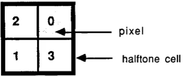
A periodic screen consists of a pattern (the halftone cell, figure 7) which is repeated in

orthogonal directions. The screen's fundamental period (the halftone cell size) is

substantially larger than the pixel interval. This results in many pixels per halftone

c e l l2 7.

p i x e l

halftone cell

Figure 7. Example of a Halftone Cell Pattern

Thresholding is performed by numerical comparison in analogous fashion to the

traditional thresholding step using high-contrast film. Dark elements occur when

l(x) + S(x) > lT. (5)

The resultant binary image, B(x), consists of a matrix of black imaging elements of one

size, and white substrate. In figure 8, the digital halftone binary structure is

• %

The fractional area coverage is altered by changing the number of imaging elements per

area A. Whereas the traditional halftone binary structure may take on any one of an

infinite number offractional areas, the digital fractional area coverage may take on only

discrete values. Hence, the average reflectance and average density of the output will be

discrete as well.

The digital-halftone process has been described for a print-black (i.e. negative)

system. Typically, the imaging element is a black dot which creates a high average

density for a high fractional area coverage. Due to the initial approach taken by the

author, the results in this paper are from a print-white system {i.e. a low average

density for a high fractional area coverage. This is evident in the results, especially in

the tone reproduction analysis. Both approaches are valid (print-black and

2.0 Digital Halftone Screen Patterns

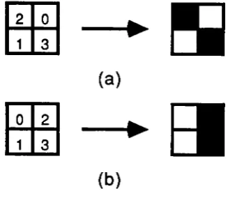
Digital halftone screens, and in particular the halftone cell pattern of the

screens, define the halftone binary structure. In figure 9, two different cell patterns

and their corresponding binary structures are illustrated for 50% fractional area

coverage. Notice the difference in placement of the two 'on' pixels.

2 0

1 3

0 2

1 3

( a )

a

(b)

Figure 9. Two Halftone Cell Patterns and Corresponding Binary Structure for 50% Fractional Area Coverage

Many cell patterns have been developed with the intent to optimize certain final

image characteristics. Following is a discussion of four screen patterns and the

characteristics they were designed to optimize. The set yields a range of binary

structures: the diamond dot s c r e e n2 8 produces a clustered-type structure which closely

resembles that of traditional halftone, the screen developed by B r y n g d a h l2 9 creates a

ringed binary structure; and the Bayer s c r e e n3 0 simulates a dispersed structure.

2.1 Diamond Dot Screen

In general, screens that produce binary structures with dispersed imaging

elements are preferred over those producing binary structures where the image

elements are clustered together. Dispersed patterns tend to be less visible3 2- There are

devices, though, which cannot properly print isolated pixels. In offset printing, for

example, a halftone screen yielding a cluster-type binary structure is used since the

clustered structure represents the minimum area that is reliably reproduced and

maintained as the press runs. Plate wear is an issue, along with the size of the imaging

element on the plate. The cluster-type structure is used even though the cell pattern is

highly visible. The diamond dot screen is an example of a clustered-dot-producing

screen.

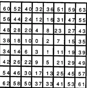
The printing industry is the largest user of the clustered-type s c r e e n3 3. The

diamond dot s c r e e n3 4 depicted in figure 10 creates a clustered binary structure. The

structure is centered about the middle of the halftone cell and the fractional area

6 0 5 2 4 0 3 2 3 6 51 5 9 6 3

5 6 4 4 2 4 1 2 1 6 31 4 7 5 5

4 8 2 8 2 0 4 8 2 3 2 7 4 3

3 8 1 8 1 0 0 2 7 1 5 3 5

3 4 1 4 6 3 1 1 1 1 9 3 9

4 2 2 6 2 2 9 5 21 2 9 4 9

5 4 4 6 3 0 1 7 1 3 2 5 4 5 5 7

6 2 5 8 5 0 3 7 3 3 41 5 3 61

Figure 10. Halftone Cell Pattern for Diamond Dot Screen

Figure 11 illustrates the binary structure produced by the diamond dot screen for 10%

through 100% fractional area coverage.

i i

10% 20% 30% _{40% 50% 60% 70% 80% 90% 100%}

Figure 11. Binary Structure for 10 %-100% (10%) Fractional Area Coverage Produced from One 8 by 8

Diamond Dot Halftone Screen Cell

2.2 Brvnadahl-tvpe Screen

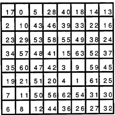
B r y n g d a h l3 5 developed a halftone screen with a ringed binary structure. Since

final image areas, Bryngdahl argues that the halftone screen cell should maximize the

length of the boundary between these areas to optimize reproduction of detail. Also, the

locations of this boundary should be distributed as uniformly as possible. To this end, he

proposes that the halftone screen cell pattern build the binary structure in the form of

rings. With a ringed shape geometry, a change in scene gray level is reflected in a

variation of the width of an annular area instead of a change in the radius of a circular

structure as in the traditional halftone case. An example of a screen based on his scheme

is shown in figure 12.

1 7 0 5 2 8 4 0 1 8 1 4 1 3

2 1 0 4 3 4 6 3 9 3 3 2 2 1 6

2 3 2 9 5 3 5 8 5 5 4 9 3 8 2 4

3 4 5 7 4 8 41 1 5 6 3 5 2 3 7

3 5 6 0 4 7 4 2 3 9 5 9 4 5

1 9 21 51 2 0 4 1 61 2 5

7 1 1 5 0 5 6 6 2 5 4 31 3 0

6 8 1 2 4 4 3 6 2 6 2 7 3 2

Figure 12. Halftone Cell Pattern for Bryngdahl Screen

The binary structure produced by a Bryngdahl halftone cell for different percentages of

B B B H K M W £.

•

80% 90% 100%

Figure 13. Binary Structure for 10%-100% (10%) Fractional Area Coverage Produced from One. 8 by 8

Bryngdahl Halftone Screen Cell

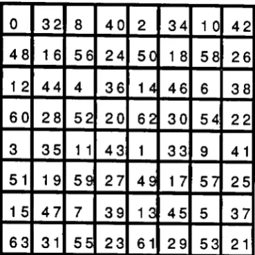
2.3 Baver-tvoe Screens

When creating his halftone screen, B a y e r3 6 attempted to minimize the

amplitude of the lowest spatial frequency of the non-zero Fourier components of the

binary structure. This minimizes halftone pattern visibility and maximizes resolution

of detail in the output image. This result is accomplished by creating the halftone image

using a dispersed filling pattern. The screen also required a square halftone-cell of size

2n (n=1,2 N). Using his optimization criteria, Bayer determined that the previous

halftone cell patterns designed by L i m b3 7 and Lippel and Kurland 3 8 were also optimal.

Judice, et. a / .3 9 developed a recurrence relationship to generate Bayer-type matrices.

Although this approach minimizes the halftone cell visibility, it has been reported to

0 3 2 8 4 0 2 3 4 1 0 4 2

4 8 1 6 5 6 2 4 5 0 1 8 5 8 2 6

1 2 4 4 4 3 6 1 4 4 6 6 3 8

6 0 2 8 5 2 2 0 6 2 3 0 5 4 2 2

3 3 5 1 1 4 3 1 3 3 9 41

5 1 _{1 9 5 9 2 7 4 9 1 7 5 7 2 5}

1 5 4 7 7 3 9 1 3 4 5 5 3 7

6 3 31 5 5 2 3 61 2 9 5 3 21

Figure 14. Halftone Cell Pattern for Bayer Screen

In figure 15, the binary structure for various fractional area coverages created by one

Bayer halftone cell is illustrated.

B S B 3 9

P ^ O rT T Tl

10% 20% 30% 40% 50% 60% 70% 80% 90% 100%

Figure 15. Binary Structure for 10%-100% (10%) Fractional Area Coverage Produced from One 8 by 8

Bayer Halftone Screen Cell

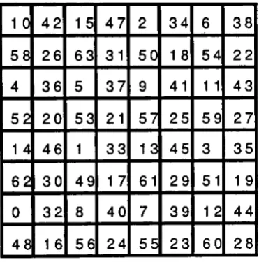
2.4 Allebach-type Screens

Allebach and Stradling4 2 developed a screen which was designed to meet Bayer's

referred to as the Allebach screen. The method for determining an optimum screen

pattern was based on Fourier analysis of the binary structure. Allebach found that the

visibility of the binary structure and poor resolution of details were due to a l i a s i n g4 3.

Through an iterative pairwise exchange algorithm, he developed the halftone cell pattern

shown in figure 16.

1 0 4 2 1 5 4 7 2 3 4 6 3 8

5 8 2 6 6 3 31 5 0 1 8 5 4 2 2

4 3 6 5 3 7 9 41 1 1 4 3

5 2 2 0 5 3 21 5 7 2 5 5 9 2 7

1 4 4 6 1 3 3 1 3 4 5 3 3 5

6 2 3 0 4 9 1 7 61 2 9 51 1 9

0 3 2 8 4 0 7 3 9 1 2 4 4

4 8 1 6 5 6 2 4 5 5 2 3 6 0 2 8

Figure 16. Halftone Cell Pattern for Allebach Screen

The binary structure from the Allebach halftone cell pattern is pictured below for

nS no

lH

10%

Figure 17. Binary Structure for 10%-100% (10%) Fractional Area Coverage Produced from One 8 by 8

Allebach Halftone Screen Cell

3.0 Objective

The objective of this experiment is to assess and compare four halftone screens

by objectively evaluating the screens' effect at the microstructural level on tone

reproduction, spatial signal reproduction, and quantization noise in the final binary

image. This is done by measuring the tone reproduction curve, the two-dimensional

Fourier Transform of a constant density patch, the degree of harmonic distortion, the

system Modulation Transfer Function (MTF), and the Wiener Spectrum (WS) produced

by each screen. The results will indicate the ability to evaluate binary output using

conventional evaluation metrics.

The comprehensive evaluation methods listed above are commonly used in

conventional reproduction analysis and are described in detail in the Section II. 1) The

level. The plot yields the contrast and reflectance range of the reproduction system. 2)

The two-dimensional Fourier Transform of a digitally halftoned uniform gray patch

yields the degree of uniformity with which the patch was reproduced, i.e. the spectral

components introduced by halftoning. 3) Total Harmonic Distortion (THD) is a sum of

the multiple frequency Fourier components created when halftoning a sinusoid. It is a

measure of the degree of non-linearity present in a system. 4) The system Modulation

Transfer Function (MTF) is derived to measure the ability of the halftoning procedure to

accurately reproduce all frequencies. An edge input is halftoned and the line spread

function is obtained by taking the derivative of the halftoned edge. In a linear system,

the modulus of the Fourier Transform of the line spread function yields the MTF of the

halftoning system. 5) Finally, noise introduced by quantization is measured by

evaluating the Wiener Spectrum (WS). The Wiener Spectrum is obtained through an

autocorrelation of the noise and a subsequent Fourier Transform.

A variety of evaluation methods for measuring final binary image

characteristics have been designed and i n v e s t i g a t e d ,4 4-4 5-4 6'4 7'4 8'4 9-5 0'5 1 -5 2 but no

where in the literature is a complete objective analysis using the methods described

Since the output from the digital halftone process is binary and highly

non-linear, it would seem that the linear evaluation tools described in the following

section, e.g. harmonic analysis, would not be applicable to digital halftoning output. However, if the output undergoes spatial averaging (similar to the action of the human

visual system or a microdensitometer scanning slit), the output may be considered

continuous and these evaluations are applicable. According to equation 1, the

two-dimensional binary output can be reduced to one dimension by spatial averaging, i.e. determining fractional area coverage. This transformation is accomplished through

halftone-cell or column averaging. In halftone-cell averaging it is assumed that the

aperture area A is equal to one halftone cell, i.e. A equals the number of pixels in a halftone cell. Therefore,

fc en = number of 'on' pixels in one halftone cell (6)

number of pixels in a halftone cell

In column averaging, it is assumed that the aperture area A is equal to one column, i.e. A equals the number of pixels in a column. Hence,

fcolumn = number of 'on' pixels in one column (7)

number of pixels in a column

Once f(x) is defined through halftone cell or column averaging, another basic

evaluation tool, the discrete Fourier transform (DFT), is utilized. The transform

decomposes f(x) into a linear combination of complex-valued coefficients which

represents the frequency make-up of f(x). f(x) and F(u) are Fourier transform pairs.

The DFT is used to compute the Fourier series coefficients, each of which is

characterized by a particular frequency. If f(x) is a sinusoid with a spatial frequency of

u0, its Fourier transform will consist of one component at the fundamental frequency. If

f(x) is the sum of two sinusoids of different spatial frequencies, the Fourier series will

contain two components, one at each of the two fundamental frequencies. Any function

can be considered as the sum of a number of sinusoids with varying frequencies and

amplitudes. The DFT is used to define the sinusoidal components present in f(x). Figure

18 illustrates the relationship between f(x) and its Fourier spectrum, F ( u ) .5 3

f(x) - l / N ^ F ( u ) e A u

a) f(x) = A

f ( x ) F ( u )

b)f(x) = Acos(2rcu X)

f ( x )

A

-A / 2 |

-u

F ( u )

| A / 2

c) f(x) = ACOS(2TC(5U 0 )X)

f ( x ) F ( u )

A / 2 1 -5u

A A / 2

5u 11

Figure 18. Relationship Between the Frequency of a Cosine Function and its Fourier Spectrum

1.0 Tone Reproduction Analysis

In traditional photography, the tone reproduction curve (TRC) is a density vs. log

(input) will produce. This concept can be used with digital halftoning as well. Instead of

log exposure, gray level is the input. After halftoning, the output image is composed of a

two-dimensional binary structure. According to equation 6, the two-dimensional binary

output can be reduced to one dimension through halftone cell averaging. Average

reflectance and average density are determined from fce||.

R = fcell

D = -log(fc en) (9)

assuming R(i) = 1.0 and R(p) = 0.0.

The T R C for digital halftoning is used to show two specific ways the halftone

screen affects tone reproduction: 1) the halftone screen cell size determines the number

of reproducible reflectance or density levels, while 2) the threshold values within the

halftone cell determine the overall contrast of the final image. In an n by m halftone cell

there are (n x m) + 1 possible gray levels, i.e. (n x m)+1 possible average reflectance or average density levels. Figure 19 illustrates the effect of halftone cell size on the

T R C . Due to the limited number of reproducible reflectance levels, the T R C is a series of

a) 2 by 2 halftone cell, 5 gray levels b) 4 by 4 halftone cell, 17 gray levels

Tone Reproduction Curve

S I 5 T

71 1C: 125 150 175 203 225 2SC Inpul gray level

c) 5 by 5 halftone cell, 26 gray levels

Figure 19. Effect on the Tone Reproduction Curve of Increasing the Halftone Cell Size

In addition to determining the number of reproducible gray levels, the halftone

screen cell alters the shape of the tone reproduction curve when a constant is added to the

4 1 61 1 5 3 9 2 1 0

8 2 1 7 3 2 4 5 2 0 4 1 1 2

1 4 3 2 1 4 2 5 5 2 2 4 1 3 3

1 2 2 1 9 4 2 3 5 1 8 4 71

2 0 _{1 0 2 1 6 3 51 31}

a) 5 by 5 halftone screen cell pattern, threshold = 256

T o n e R e p r o d u c t i o n C u r v e T o n e R e p r o d u c t i o n C u r v e

Additive C o n s t a n t s : -60. 0, +60 Multiplicative Constants .2. .6. 1.0, 1 4 . i s

input gray level input gray level

b) add constant to screen c) multiply screen by constant

Figure 20. Effects on T R C of Adding or Multiplying a Constant to the Screen Cells' Values

The shape of the T R C remains unchanged but is shifted along the x axis (figure 20b)

when the halftone screen cell pattern is changed by adding a constant. The contrast or

slope {(y2-y-|V(x2-Xi)} ° ft n e curve changes (figure 20c) when the halftone screen

2.0 Tone Uniformity Analysis fAliasing)

Whereas the T R C yields results about contouring and contrast, it shows nothing

about the uniformity of a constant gray level area. Fourier analysis of the binary

structure is one method of e v a l u a t i o n5 4'5 5-5 6-5 7-5 8. Figure 21 illustrates the

degradation in the Fourier domain that occurs when a 50% gray-level continuous image

is halftoned. Degradation, in this example, is defined as the addition of spatial

frequencies due to halftoning.

2D F F y

a) digitized image

b) quantized form

When the digitized form of a continuous tone image of one gray level (figure 21a) is

Fourier transformed, the resulting function contains one zero-order term and no

frequency components. If that image is halftoned, the Fourier transform of the binary

structure indicates that frequency components have been introduced. The zeroth-order

spectrum of the binary structure is that of the quantized original image while the other

spectra correspond to distortions5 9- These distortions are due to an interaction between

the original scene and thresholding steps that give rise to new frequencies. If low

enough, these lower frequencies will be perceived as a l i a s i n g6 0. Aliasing describes the

low frequency components of the Fourier transform not present in the digitized or

continuous image but that appear in the halftone image. The visibility of these artifacts

may be reduced by choosing a spatial arrangement within the halftone cell which

minimizes all non-zeroth-order terms and places them at less-visible higher

frequencies6 1. By analyzing the spectrum created by halftoning, the degree of aliasing

produced by different screen thresholding patterns may be compared.

3.0 Harmonic Distortion Analysis

Signal-reproduction characteristics are determined by the ability of the digital

halftone screen to accurately reproduce an input signal of a particular spatial

configuration. Harmonic analysis can be used to measure and compare the amount of

3.1 Total Harmonic Distortion

If a system has two one-dimensional inputs, f^x) and f2(x), and uses an

operator, B , such that

In digital halftoning, f1 (x) can be assigned the input image value, f2(x) can be

assigned the screen value, and B is the thresholding operator. If the system is linear,

the 1 or 0 resulting from thresholding the image value, plus the 1 or 0 resulting from

thresholding the screen value will equal the 1 or 0 resulting from thresholding the sum.

A metric suitable for evaluating linearity is THD. B { fi(x) } -f l l( x )

B {f2(x) } = g2(x) (10)

it is considered linear if

B { WxJ + f g M } = B { M x ) } + B { f2(x) }

= 9l(x) + g2(x) (11)

THD is the square root of the ratio of the sum of the squares of the harmonic amplitudes

for all non-zero frequencies except the fundamental frequency, divided by the square of

the amplitude at the fundamental frequency.

The input form of interest is the sinusoid. After halftoning, the sinusoid has two

dimensions. A s already discussed, this two-dimensional image can be converted to one

dimension, f(x), through column averaging, fC 0|u m n (equation 7), which is analogous to

scanning with a slit on a microdensitometer. The discrete Fourier transform (DFT) is

then used to compute the Fourier Series coefficients of f(x). THD is determined from the

DFT results.

If f(x) is linear and has been reproduced as a perfect sinusoid, F(u) will have

one non-zero harmonic component associated with its fundamental frequency. If

distortions are introduced through processing, f(x) will not be a perfect sinusoid and

F(u) will contain non-zero components at frequencies other than the fundamental. THD

analysis (equation 11) uses this result to measure the degree of process linearity. If

THD equals zero, there are no harmonic amplitudes beyond the fundamental frequency

and the system is linear. A s the process becomes non-linear, THD will increase.

In this experiment, the processing referred to in the above discussion is

halftoning. Non-linearities in f(x) are introduced in the screening and thresholding

steps. THD is a metric for comparing the ability of the four screens to linearly

3.2 Fisher's Test of Harmonic Significance

In digital halftoning, noise is introduced by quantizing a continuous-tone image to

a one-bit image. This noise may be sufficient to render the results of the THD analysis

uncertain. Even if there are no periodic components in a random series of points, some

of the amplitudes obtained by harmonic analysis would be greater than others, simply

due to random fluctuations of the Fourier components.6 2 Since the output of digital

halftoning will contain noise and signal, a method is needed that will detect signal apart

from noise.

Fisher's test of significance in harmonic analysis is designed to measure just

that.6 3 It is used to determine the plausibility that a certain amplitude represents a

real periodicity.6 4 The test was developed by F i s h e r6 5 and generalized by Grenander and

Rosenblatt6 6. The test method determines the probability that the largest of the

harmonic amplitudes, given in a normalized form with respect to the data, is the result

of randomness of the d a t a .6 7 If the normalized amplitudes of the harmonics g|<,

k=1,2 m, is arranged in decreasing order, and gr is the rth largest term of this

m-1 P ( gr> 9 ) = ml y ( i )J ~r (1-jg r)

= amplitude of the harmonic component for k = 1,2, ... m

gk = normalized ck, ck 2

gr = ordered g.

m

I Cj2

J = 1 J

L = largest-integer, | 1/g r | for 1 / g p

= m for 1/g r > m

(13)

S h i m s h o n i6 9 calculated a table of critical values for various parameters.

Fisher's test is designed to be used based on certain assumptions that noise is

random. Since quantization noise may not meet these requirements, a test must be

performed on Fisher's method to determine its robustness.

4.0 System Modulation Transfer Function Analysis

The second input signal of interest is the edge. Column averaging of the processed

image, B(x,y) will yield the equivalent of an edge trace, e(x). For a linear system, e(x)

is actually the result of a perfect edge (l0(x)) convolved with a point spread function

(h(x)) of the processing system. Convolution will be discussed in the sub-section 5.0.

A one-dimensional system convolution is illustrated in figure 22 (* indicates

= =>

h ( x ) e ( x )

Figure 22. Effect on l0(x) of the System

Point Spread Function, h(x)

The derivative of an edge trace is the line spread function (l(x)) and the Fourier

transform of the line spread function is the optical transfer function, L(u).

d ( e ( x ) )

dx

FFT l(x)

L(u) is complex-valued and is of the form

L ( u )

(14)

L(u) = R(u) + il(u)

R = real portion of L(u) I = imaginary portion of L(u)

(15)

The Modulation Transfer Function (MTF) is the modulus of L(u), and is always positive;

MTF(u) = V (L(u))2

= V R2 + |2 ₍₁₆₎

L(u) is equivalent to H ( u )7 0, the system MTF. This approach to finding the system MTF

is valid for a linear, shift-invariant (LSI) s y s t e m7 1.

If an edge (l0(x)) is perfectly reproduced to e(x), then imaging is perfect and the point

spread function (psf) is a delta function. The resultant MTF will contain constant

amplitudes over all frequencies. Any degradation in l0 (x,y) caused by the psf of the

system will cause the system MTF to deviate from a constant value. Variations between a

perfectly and imperfectly reproduced edge are pictured in figure 23.

a) perfectly reproduced edge

— A s l o p e = 0

derivative FFT

e ( x ) l(x) = psf L(u) = |H(u)|

b) imperfectly reproduced edge 0 derivative FFT

Figure 23. MTF Difference Between a Perfectly and Imperfectly Reproduced Edge

A is commonly normalized to 1.0 at u = 0. If H(u) is less than 1.0, the system is unable

to completely reproduce the Fourier component at frequency u. A value greater than 1.0

indicates that the system amplifies components with that frequency.

5.0 Quantization Noise Analysis

An error is introduced when the infinite number of input gray levels are forced into a

finite number of integral halftoned output gray levels. If the normalized original

continuous-tone image is considered the actual image gray level, and the normalized

column average of the quantized form is considered the processed gray level, then the

Grayprocessed = G r a ya c t u a| + noise

noise = G r a ya c t u a| - G r a yp r o c e s s e d (18)

An example of the effect of processing parameters on noise is seen in the influence of the

size of the halftone-screen cell. A s shown in section I, the tone-reproduction curve

becomes smoother and more continuous as the screen-cell size increases, i.e. there is less error due to quantizing. Hence, larger matrices result in less noise.

An estimate of the amount and type of noise is needed to evaluate the effect of the

screen function on noise. Useful evaluation tools are the autocorrelation, Cx x, function

and its Fourier transform, the Wiener spectrum, WS(u). The autocorrelation function

measures the correlation between two points in the image. For a discrete random

process, the autocorrelation function estimate is defined as:

N

(19)

t=1

N = number of data points

f(xt), f ( xt + k) = value of f(x) at x=t or x=(t+k)

The autocorrelation at any value of the shift, k, is just the average of the product of the

random process with a copy of itself shifted by k. The units of Cx x( k ) are the squared

As already stated, the autocorrelation function and the one-dimensional power

spectrum are Fourier transform pairs.

I - I2T C U X ,

WS(u) =J C (x)e dx

_ X X

C (x) =1 W S ( u ) e '2 7 l u xd u xx

(20)

The Wiener spectrum is a power spectrum of noise and has units of area multiplied by

the squared units of f(x).7 2 If no noise were added to an image, the autocorrelation

( Cx x) and the Wiener spectrum (WS) of the noise would not exist. If periodic noise

were added, the W S would contain a set of components which described the spectral

distribution of noise power. By evaluating the Wiener spectrum, the type and frequency

Figure 24 summarizes the halftone procedure and evaluations used in this

experiment. I0(x,y) is the original continuous tone image that is digitized to l(x,y), an

eight-bit image of 256 levels. I0(x,y) is one of three inputs: 1) a large constant gray

level patch, 2) a sinusoid, or 3) an edge.

1) constant gray l0(x.y) = gray level

2) sinusoid l0(x.y) = a+Acos(2nx/p)

a=constant A=amplitude x=distance p=period

3) edge l0(x,y) = Step(x)73 (21)

Quantization proceeds as follows:

l(x,y) = nint( l0(x,y)) (22)

where nint indicates the nearest integer. Once the digital image is formed, the halftone

screen is added and the sum is thresholded to produce a bitmap. This section describes

1.0 Halftone Screens

The halftone cell size and the halftone cell scale are two variables of the screen

that are fixed prior to halftoning. Following is a discussion on the levels that were

chosen for each.

1.1 Halftone Cell Size

The screens are made from four different halftone cell patterns described in

Section I: Diamond Dot, Bryngdahl, Bayer, and Allebach. The size of the halftone cell

determines the number of reproducible gray levels; an n by m cell yields (n x m)+1

levels. The smaller halftone cells tend to exhibit false contouring due to the limited

number of gray levels available. A s was shown in figure 19a, the quantized values in a 2

by 2 cell have only five output gray levels in which to fall. This causes the output image

to make large jumps in output gray level, while there may only be small jumps in input

gray level. As the size of the halftone cell increases (figures 19b, 19c), the possible

number of gray levels increases and subsequently the tone reproduction curve becomes

smoother and more continuous.

At first, it might seem that a large halftone cell would produce the best result.

This is not necessarily so because there is a tradeoff between the level of reproducible

detail and the size of the halftone cell. When the halftone cell size is increased, the

amount of detail decreases because there are less halftone cells per image of a given size.

J a r v i s7 4 investigated the subjective effects of the halftone screen cell size and

found that a 16 by 16 matrix does not produce a noticeably different output from the 8

by 8 matrix. He concluded that the image data noise is usually greater than four

intensity units, the additional fineness in the thresholds of the 16 by 16 matrix does not

significantly affect the output images. He finds that digital halftone screens made with

an 8 by 8 halftone cell (65 gray level capability) is the optimum halftone screen to use

as it balances the false contouring created by 'small' cell sizes with the loss of detail

created by 'large' cell sizes.

An additional argument for an 8 by 8 halftone cell is found in the properties of

the human visual system. A typical maximum achievable reflectance in a reproduction

is 9.5 in the Munsell Lightness S c a l e7 5. The minimum is approximately 1.5-2.0. This

gives a reproducible range of approximately 8 M u n s e l l7 6 values. Since a

just-noticeable difference Qnd) in lightness has a Munsell value of .1, the number of

perceptible gray levels in a reproduction is about 8/.1, or 80. It has already been

discussed that there are (n x m) + 1 gray levels in an n by m halftone cell. An 8 by 8

cell yields (8 x 8)+1, or 65 gray levels. This approaches the 80 gray levels

perceivable by the eye. The next size, a 16 by 16 matrix, yields 257 gray levels which

is over three times the number of perceivable levels. This requirement and a limit of a

2n square cell size required by Bayer's criterion resulted in an 8 by 8 halftone cell in

1.2 Halftone Cell Scale

Once l(x,y) is formed, it is added to the properly scaled screen pattern, S(x,y).

The effect of altering the values within a halftone screen by addition or multiplication is

considered in the discussion of evaluation methods. The 8 by 8 halftone cells described

in section I have 65 values ranging from 0 through 64. This range must be expanded to

cover the range of l(x,y). The expansion is done by simply determining the desired

range (0 through 255), the current range (0 through 63), and the ratio between them

(255/63=4.05). If this cell range expansion step is not performed, many pixels will

be set to zero in the thresholding step instead of being set to one, i.e. I(x,y) + S(x,y) will be too small. Each threshold value within the halftone cell is multiplied by 4.05 to

obtain a range of screen values from 0 to 255.

The halftone cell is then repeated as many times as necessary to create a screen

the size of l(x,y). For the constant gray level patch the screen is the size of the cell, for

the sinusoid it is repeated 16 times for a 128 by 8 pixel screen, and for the edge it is

repeated four times for a 32 by 8 pixel screen.

2.0 Halftone Threshold Value

The range of the image is set at 8-bits (0 through 255), and the range of the

screen is equivalent (0 through 255). When the screen is added to the image, the

resultant sum has a possible range of 0 through 510. Figure 25 illustrates the result of

A 5 1 0

2 5 5 threshold value

t o

image + screen range

Figure 25. Determining the Threshold Value

A threshold value should be chosen such that an image value at 50% of the image

range (127) will reproduce with .5 fractional area coverage. This occurs when the

threshold is chosen at the half-way point of the image + screen range, or at 255.

3.0 Test Patterns

Three test patterns are used in this study. The first of interest is the constant

gray level patch. For the patch, an 8 by 8 matrix of one gray level is formed. This form

is useful for two analyses. For the tone-reproduction curve (TRC), 256 of these

patches are produced, with each having a constant value between 0 and 255.

For the tone uniformity analysis ten matrices are formed. The ten patches

contain a constant gray value that when processed yields ten different fractional area

coverages (,..10 through 1.00 in ...10 increments).

The sinusoidal input form l(x,y) is a 128 sample (x) by 8 line (y) matrix

variables used to describe the sinusoid. Figure 26 illustrates how one line of the

sinusoidal input is created.

1 2 3 4 / 63 64 65 66 6 7 ' 126 127 128 pixel (x)

Figure 26. Components of One Line of a Quantized Sinusoid, l(x) = a + Acos(2rcx/p)

The line y=1 is then repeated eight times to produce a 128 by 8 matrix. The period of

the sinusoid is described in halftone cells per cycle. For example, if the halftone cell is

eight pixels long, and a sinusoid is 64 pixels long, the sinusoid is described as (64

pixels per cycle) / (8 pixels per halftone cell), or a period of 8 halftone cells per cycle.

Each of the sinusoids was created as a cosine with an average gray level (a) of 128. The

peak gray level is placed at x=1 for position 1 (see figure 26) and the period is 2, 4, 8,

or 16 halftone cells per cycle. The sinusoidal period is limited to these values due to the

In addition to period and amplitude, another variable in the halftone process is

the phase of the sinusoid, i.e. the position of the first sinusoidal gray level peak with respect to the position of the first halftone cell. Position 1 indicates that the first

halftone screen cell position is placed at the peak cosine level, at x=1. Position 2

indicates that the first cell position is placed at the position following the peak cosine

level, x=2, and so on. The effects of a sinusoid at position 9 is the same as position 1

because the halftone cell is periodic within the screen and repeats every 8 pixels in the

x direction. It is therefore necessary to investigate only the effects of setting the

sinusoid at positions 1 through 8. In figure 27. the difference between a sinusoid at

position 1 and position 2 is illustrated for one dimension. Pixels one through ten are

Screen at position one - sinusoid

2 3 4 5 6 8 7 9 1 0

l ( x ) 2 5 5 2 5 4 2 5 3 2 5 2 2 5 1 2 4 9 2 4 7 2 4 4 2 4 0 2 3 5

+

1 • •

S ( x ) 2 5 5 0 1 6 1 2 8 3 2 1 4 8 2 0 9 2 | 2 5 5 0

halftone

c e l l . . | position I 1

one halftone cell

3 4 5 6 7 8 I 1

I

Screen at position two sinusoid

3 4 5 6 8 7 9 1 0

l ( x ) 2 5 5 2 5 4 2 5 3 2 5 2 2 5 1 2 4 9 2 4 7 2 4 4 2 4 0 2 3 5

+

• • S ( x )

9 2

1 I

1 1

halftone c e l l

position ₈

I

I

h

one halftone cell

4 5 6 7 ₃

1

1

Figure 27. Effect of Changing Sinusoidal Peak Gray Level Position, One Dimension

Shifting the sinusoid produces the same effect as keeping the peak gray level of the

The levels chosen for the three sinusoidal variables are as follows: period (p) at

2 , 4 , 8, or 16 halftone cells per cycle, amplitude A at 10 through 120 in increments of

5, and position at one through eight. This covers the range of possible settings.

The third input form, an edge, is created in a similar fashion to the sinusoid. It

is a matrix of 32 samples (x) by 8 lines (y) and l(x,y) reflecting the gray level for

each side of the edge. Figure 28 illustrates how one line of the edge input is created.

y = 1 1

255

255

i

gray level

^ I I ^ 1

' 1 5 16 17 1

1 2 3 4 ' 1 5 16 17 18 1 9 ' 30 31 32 pixel (x)

Figure 28. Components of One Line of a Quantized Edge, l(x) = Step(x)

This 32 sample line is repeated to create a 32 by 8 matrix. The lower gray value, or

x=17. Average gray is kept constant at 128 throughout the experiment, while contrast

ratio and halftone cell position are altered.

Again, the first cell position of the edge is defined with respect to the position of

the halftone cell. The edge is placed somewhere between x=17 and x=24 which is in the

center of the image and covers the range of one halftone cell. For position 1, the edge is

placed at x=17, the first position within a halftone cell. Position 2 indicates that the

edge is placed at the second halftone cell position, x=18, and so on. Position 9 is a repeat

of position 1, therefore only positions 1 through 8 are investigated. A one-dimensional

example is shown in figure 29 which illustrates the difference between an edge at

position 1 and position 2.

Average gray = ( g r a ym a x + g r a ym i n) / 2 (23)

1 7

Screen at position one - edge

1 8 1 9 2 0 21 2 2 2 3 2 4 2 5 2 6

l ( x ) 1 2 5 5 2 5 5 2 5 5 2 5 5 2 5 5 2 5 5 2 5 5 2 5 5 2 5 5

+

1

S ( x ) I 2 5 5 0 1 6 1 2 8 3 2 1 4 8 2 0 9 2 2 5 5 0

_ one halftone cell halftone

c e l l . |

position | 1 2 3 4 5 6 7 8 | 1

I

1 7

Screen at position two - edge

1 9 2 0 21 2 2 2 3 2 4 2 5 2 6

l ( x ) 1 2 5 5 2 5 5 2 5 5 2 5 5 2 5 5 2 5 5 2 5 5 2 5 5 2 5 5

+

•

S ( x ) 9 2 | | 2 5 5 0 1 6 1 2 8 3 2 1 4 8 2 0

9 2

I

I

halftone c e l l

position ₃

I

1

h

one halftone cell

4 5 6 7 _B

I

1

1

Figure 29. Effect of Changing Edge Position One-dimension

Shifting the edge position produces the same results as keeping the edge position constant

The levels chosen for the two variables are as follows: contrast ratio at 255

(255/1), 125 (254/2), 80 (253/3), 50(250/5), 30 (248/8), and 10 (230/23),

and positions at one through eight. The contrast ratios are approximate; they were

chosen to keep the average gray level at 128 and still produce a representative contrast

IV. RESULTS

Typical test results are shown in this section. A complete set is found in the

appendices and a discussion on these results is found in Section V. Four sets of images

are included in this paper to aid the reader in understanding the visual effects of the

screens on a scene. The first consists of an image of a person and is found on the next

four pages. The other two sets, 'kid' and 'tree', are found in Appendix V. The original

images are 512 pixels by 512 pixels, quantized to 256 gray levels. After halftoning,

they are printed with a laser binary-output device. Each halftone pixel is made of 16 by

16 laser-sized pixels. The images are included only for reference and are not used in

the evaluation process.

Following these images is an illustration of the binary structure each screen

produces at different percent coverages. Note that the percentages are approximate and

D i a m o n d Dot

• • • • • » # « . • • • . * - - • • • • • • • • • • • » » » • - » •

••••**»*•». • -• -• -• » -• * * . . * - . , . .

« » »

-• » . * * » -• -• -• -•

B r y n g d a h l

i>t>t>f>t>t>«>«>o<><»t>ec>o t>6t>t>t>t>t>c>t>p<»t>«>t>«>

t> t> t» «• e> t> t> t> t> t> tv&« o o

O *S <> O <• «• O t> «> t>

c-e>tx>f>»>f>t>p<vt>e»«>t>o. t> f> «• t> V P €• O f> o t> O t> t> t» t» <**t»op«>t>a cit-s'<»•>«••> <-t>ot>o<>t>ot!o

e>e»e><»t>t>o <>*>«> o c * o (><»<»yt>c»o c o o^ e o

p06t>C>t>t>Ot> o t) o o

P<» C» t>t? O O O O O O T.

oooooot>&C'vfrfrC*5555s

f>c • oooooOC,€*ft555555

f>o o o o o o ^ t>c»55*^*55S

ooo'>oopc^555 555s OP c> '-• •:• o ">*5555555S

>••.> • ''°^S^£JSSS

',>•>o?<>222^^M

" ^ * ^ ^ 5 ^ ^ ^ q <>o-. --:>r->*555££x£2255

Binary Structure

10% 100% fractional area coverage

Diamond Dot

H

O

10% 20% 3fj% 40o/o 50o/o 60o/o 70o/o 80o/o 9 0 % 100o/o

B r y n g d a h l

B B B H H H H

F-10% 20% 30% 40% 50%

1

—i *

60% 70% 80% 90% 100%

no

B a y e r

X X

10% 20% 30% 40% 50% 60% 70% 80% 90% 100%

A l l e b a c h

1.0 Tone Reproduction Analysis

Following are tone reproduction curves (average output reflectance as a function

2.0 Tone Uniformity Analysis (Aliasing)

A complete set of plots for this part of the experiment are found in Appendix I.

The following page illustrates the Fourier transforms for 40% fractional area coverage.

For these plots and those found in the appendix, the binary structure with a certain

fractional area coverage and its corresponding two-dimensional Fourier transform plot

is illustrated for four screens. The plots for 10 fractional area coverages from 100% to

10% in 10% increments are included. Since the digital representation of the binary

structure is a real function with no symmetry, its Fourier transform is hermitian (real

part is even, imaginary part is odd). Since a hermitian function is conjugate

symmetric, F(5) = F*(-5), only two quadrants of the two-dimensional Fourier

3.0 Harmonic Distortion Analysis

A complete set of THD plots are found in Appendix II. The following page

illustrates the plots for position 1. For these plots and those found in the appendix, the

two-dimensional plot of THD as a function of frequency and amplitude of the input

sinusoid at a certain position is illustrated. The results of four screens for positions 1

through 8 are. included. The n axis corresponds to frequency, 1/2n cycles per halftone

cell. n=1 is the highest spatial frequency (1/2 cycles/halftone cell), andn=4isthe

lowest spatial frequency (1/16 cycles/halftone cell). The uniform n-intervals do not

correspond to a uniform spacing in spatial frequencies. All data points are placed on a

THD scale of 0 to 15 to show their relative values across the screens. This analysis did

not include Fisher's test of Harmonic Significance as it was not found to be robust under

the conditions of this study. A detailed discussion of the robustness test is found in

4.0 System Modulation Transfer Function Analysis

The plots of both the derivative and modulus of the edge traces are found in

Appendix III. The following three pages illustrate the derivative and modulus for input

sinusoids at position 1. For these plots and those found in the appendix, all four screens

are plotted on the same set of axes with each screen offset on the y axis. This was done to

facilitate comparison of the effects of the screens on MTF for a given set of parameters.

The offset changes with contrast. The lowest plot (diamond dot) is always placed at the

correct level. Plots for the other screens are offset from each other by constant values.

For example, the derivative for Bayer at contrast=125 is offset from diamond dot by .5,

Allebach is offset from Bayer by .5, and Bryngdahl is offset from Allebach by .5. The

modulus is offset by the same amount at contrasts 25. At contrast=80, though, the

modulus for each screen is offset by 1.0. The amount of offset for each case is obvious

from the plot. Included in the appendix are six sets of plots corresponding to positions

1, 2, 4, 6, and 8. FLED is an abbreviation for 'Fourier transfer of a line edge

LT)

in

CM

O l —

LJ _{_j!}

in

i °

CO

lb

3 U

o

CD < CD Q

1 1

T LT)

i

J

i

o rsj

o f

-_ j ; m

n- E L !0 0

I i I 1 .2 0 Frequenc y iLu s o f contrast" ] j 1 1 1

1 1 I

a ~> •

4i

0 —>

1

1 1

1 — L _

o w

0

a.

• O

- °

S'Z S'Z Z S'l

s n - | n p o n

S'D o c m rx L

m < ffi o

y \ [

!> y

r'

i — , •

V E 2

U c o m CM o SI

0 g

D C

0 —

'r

*- — CO Q

CD < CD Q

S ' l I S'O x p / f ( X ) e 6 p e j p

I I

^ " CO Q

" (U Q

DQ < CQ Q C Q < C Q O

5.0 Quantization Noise Analysis

The autocorrelation and Wiener Spectrum of the sinusoidal input are found in

Appendix IV. The following two pages contain results for an input sinusoid of 1/16

cycles per halftone cell frequency and 100 count amplitude. For these plots and those

found in the appendix, the autocorrelation function and Wiener Spectrum were

determined for four frequencies and three amplitudes at position one. This yielded

2 plots x 4 screens x 4 frequencies x 3 amplitudes = 96 plots. The same Wiener

spectrum distributions were found for different input sinusoidal frequencies and

amplitudes for a given screen. For brevity, just one set of plots is included for a

sinusoidal input (frequency = 1/16 cycles/halftone cell, amplitudes 00, 50,10

pixels), with the other frequencies described in the next section. The plots for an edge

1.0 Tone Reproduction Analysis

The tone reproduction curve (TRC) is a plot of average reflectance obtained by

halftoning a constant input gray level. It is used to illustrate the effects of the halftone

screen on final image tonal characteristics, namely 1) the number of available average

reflectance levels, and 2) the overall contrast of the final image.

The properties of the halftone screen that were expected to influence tonal

characteristics were the halftone cell size, and the actual values within the halftone cell.

As the cell is 8 pixels by 8 pixels in size, (8 x 8)+1 = 65 reflectance levels were

expected in the T R C . Since there are fewer output levels (65) than input levels (256),

more than one input gray level will produce the same average output reflectance. This is

expected to create a curve increasing in a step-wise fashion.

The four halftone screens were designed to produce a 0.0 to 1.0 average output

reflectance range through cell value scaling described in Section III. This means that the

T R C s are linear in a step-wise fashion. The uniform difference in consecutive cell

values produces the same increase in output values for a given increase in input values

(eg. when discounting the step characteristic, a 10 count change in input gray level will

always yield a .04 change in average output reflectance). Since the properties that

define final image tonal characteristics (halftone cell size and values) are the same in

As was expected, the curves are identical. The tonal reproduction capabilities of

the halftoning process are maximized by the screens' design as a full output reflectance

range, 0.0 through 1.0, is created by a full input gray level range, 0 through 255. The

T R C is step-wise linear, producing a contrast of 1.0/255.0. There are 65 average

reflectance levels.

2.0 Tone Uniformity Analysis {Aliasing)

Since the four tone reproduction curves are identical, a given input gray level

will produce the corresponding average reflectance independent of which screen was

used. From this result, one might think that all four screens produce the same image

tonal characteristics. While this is true for average reflectance and overall contrast, it

is not true for tone uniformity. The binary structure produced by each of the four

halftone cells for an equivalent fractional area coverage (Section IV) illustrates this

point.

Fourier analysis of the binary structure is used to evaluate uniformity. The

frequency components introduced to a continuous-tone image through halftoning are seen

in the modulus of the Fourier transform of the digital binary structure. The

zeroth-order term of the transform corresponds to the average tonal value of the

quantized original tone. Any other spectral components indicate that unwanted frequency

components were added by processing. The components present near the zeroth-order

term in the transform indicate that low frequencies are present in the halftoned patch

at higher frequencies, the halftoned patch is less likely to exhibit aliasing and the

'constant tone' area will appear more uniform.

Predictions about the amount of aliasing introduced by each screen can be made

by examining the placement of the cell values within each halftone screen. This indicates

the type of binary structure created by each screen. As fractional area coverage

increases, the binary structure created by the Diamond Dot screen increases in a

clustered pattern. This low frequency pattern is believed to be an alias candidate.

Although it differs from that created with the Diamond Dot screen, the binary pattern

from the Bryngdahl screen is believed to also cause aliasing. It's concentric ring pattern

has a low-frequency cluster in the center, although its outside ring may also add some

higher frequency components. Both the Bayer and Allebach screen create a dispersed,

high frequency binary structure. It is expected that these two screens will produce less

aliasing than the Diamond Dot and Bryngdahl screens, although no prediction is made

about which screen produces the le