Recent developments of copula based models to handle missing data of mixed type in multivariate analysis

(1)

Recent Developments of Copula-based

Models to Handle Missing Data of

Mixed-type in Multivariate Analysis

Jiali Wang

December 2018

Supervisors: Dr. Bronwyn Loong, Dr. Anton Westveld,

Prof. Alan Welsh

A thesis submitted for the degree of Doctor of Philosophy

(2)

(3)

For my beloved family. I appreciate their company and support throughout the

(4)

(5)

Declaration

The work in this thesis is my own except where otherwise stated.

(6)

(7)

Acknowledgements

I would like to thank our Research School of Finance, Actuarial & Statistics for

providing me an impressive opportunity for doing research, meeting prestigious

researchers and enjoying all the facilities.

A heartfelt thanks to my supervisor Bronwyn Loong who has always guided me

with great patience, and it has always been enjoyable to be her research assistant,

tutor and PhD student. I am grateful for working with Anton Westveld, who is a

passionate Bayesian, detailed mentor, and he always exposes me to

state-of-the-art methodologies. I would also like to say a warm thank you to Alan Welsh who

is a myth of knowledge and a respectful mentor; he has always been inspiring me

at all stages of my PhD studies.

It has been a pleasure to work harmoniously with the colleagues and fellow

students at RSFAS. I gained a lot from discussing research problems with Hanlin

Shang and Le Chang. How wonderful it is to develop friendship with my peers,

and have Yuan Gao and Yuguang Ipsen as my officemates. I am also eternally

grateful for my internship supervisors Teresa Neeman, Stephen Haslett at ANU

statistical consulting unit, and Daniel Elazar and Bernadette Fox at Australian

Bureau of Statistics for passing their valuable consulting and industrial

experi-ences to me.

Last but not the least, I own a big thank you to my mother and father who

provide my unconditional love and support me through difficult time. I am so

pleased to be accompanied by my soul mate Bomin Jiang over the years who

always cheers me up and helps with my research.

(8)

(9)

Abstract

In this thesis, we propose innovative imputation models to handle missing data of

mixed-type. Our imputation models can handle 1) multilevel data sets through

random effects; 2) heterogeneity in a population by specifying infinite mixture

models; and 3) a large number of variables using graphical lasso methods. Two

clinical data sets, a randomised control trial of acute stroke care patients and

a survey of menstrual disorder among teenagers, are used for the real data

ap-plication examples, although we believe that the proposed methods can also be

applied to other data sets with similar structures.

In Chapter 2, we propose a copula based method to handle missing values

in multivariate data of mixed type in multilevel data sets. Building upon the

extended rank likelihood approach combined with a multinomial probit model

formulation, our model is a latent variable model which is able to capture the

relationship among variables of different types as well as accounting for the

clus-tering structure. Our proposed method is evaluated through simulations using

both artificial data and the acute stroke data set to compare it with several

con-ventional methods of handling missing data. We conclude that our proposed

copula based imputation model for mixed type variables achieves good

imputa-tion accuracy and recovery of parameters in some models of interest, and that

adding random effects enhances performance when the clustering effect is strong.

In Chapter 3, we consider an infinite mixture of elliptical copulas induced by

a Dirichlet process mixture to build a flexible copula function as the imputation

model. A slice sampling algorithm is used in conjunction with a prior parallel

(10)

tempering algorithm to sample from the infinite dimensional parameter space and

to overcome the mixing issue when sampling from a multimodal distribution.

Us-ing simulations, we demonstrate that the infinite mixture copula model provides a

better overall fit compared to their single component counterparts, and performs

better at capturing tail dependence features of the data. The application of this

model is also demonstrated using the acute stroke data set.

In Chapter 4, we propose a Gaussian copula model with a graphical lasso

prior to analyse the conditional associations among 100+ questions in a study

of menstrual disorder among teenagers. Our data come from a large population

based study of menstrual disorder in Australian teenagers conducted in 2005 and

2016 respectively. We also compare cohort differences of menstruation over the

11-year interval and use the model to predict girls with a higher risk of developing

endometriosis. The model is based on the model proposed in Chapter 2, but

with a graphical lasso prior to shrink the elements in the precision matrix of the

Gaussian distribution to encourage a sparse graphical structure. The level of

shrinkage is adaptable from the strength of the conditional associations among

questions in the survey. We find that menstrual disturbance is more pronouncedly

reported in 2016 than a decade ago, and the questions in the questionnaire form

(11)

Abbreviations and Notation

Abbreviations

CDF Cumulative Distribution Function

DP Dirichlet Process

DPM Dirichlet Process Mixture

FCS Fully Conditional Specification

ICC Intra-Class Correlation

JM Joint Modelling

MAR Missing at Random

MDOT Menstrual Disorder of Teenagers

MCAR Missing Completely at Random

MCMC Markov Chain Monte Carlo

MI Multiple Imputation

MSE Mean Square Error

NMAR Not Missing at Random

QASC Quality in Acute Stroke Care

Notation

(16)

y= (y1, ..., yp) All vectors are written as row vectors.

0p Denotes a zero vector of length p.

Ip Denotes an identity matrix of dimension p.

Φp Cumulative distribution function of the p-variate

nor-mal distribution. When the subscript is omitted as Φ,

it refers to the univariate normal cumulative

distribu-tion funcdistribu-tion.

δ(a,b) Indicator function of the subset (a, b). When the

sub-script reduces to a single number, it refers to the Dirac

(17)

List of Figures

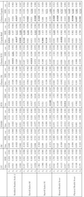
2.1 Trace plots of the marginal correlations among the four outcome

variables in the original QASC data set. . . 48

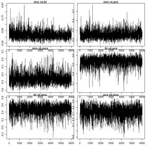
3.1 Dirichlet Processes generated by stick breaking construction, with

G0 =N(0,1), M = 1,10,100 respectively. . . 56

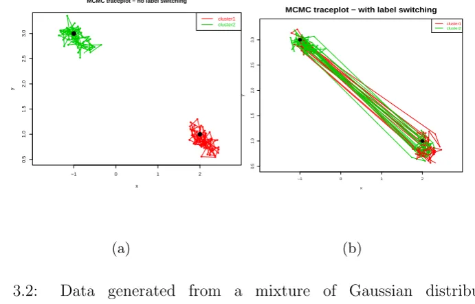
3.2 Data generated from a mixture of Gaussian distributions: 1₂N((−1,3), I2)+ 1

2N((2,1), I2). The figures show the trace plots of the mean pa-rameters in a MCMC sampler when (a) implementing a slice

sam-pling algorithm of DPM alone, and there were no label switching

between two modes; (b) implementing a slice sampling algorithm

with prior parallel tempering with 4 chains, and label switching

occurred between the two modes. . . 64

4.1 Directed acyclic graph of our proposed model. . . 88

4.2 Graphic representation of conditional dependence among the

ques-tions in the MDOT data set, with those isolated quesques-tions removed

from the graph. Edges in red denote positive relationships and blue

denote negative relationships. Questions from different sections in

the questionnaire are plotted with different colors. . . 100

4.3 Histogram (and density) of the predictive scores of endometriosis

from posterior predictive samples for each person. The scores for

the 6 girls with endometriosis were marked in solid triangles. . . . 107

(18)

4.4 Trace plots of two parametersω12 =−0.918 in the upper panel and

ω13= 0.067 in the lower panel with t=10−1,10−3 and 10−5 respec-tively. The true parameters are superimposed as the horizontal

lines. . . 112

A.1 Trace plots and ACF of the parameters in Γ and Ψ matrices under

the marginal and conditional constraint. . . 119

A.2 Trace plots of the five parallel chains and ACF of the first chain of

(19)

List of Tables

2.1 Summary of variables in the QASC data set . . . 24

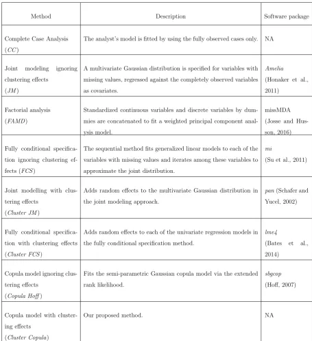
2.2 Summary of the eight methods to handle missing data used in

simulations. . . 37

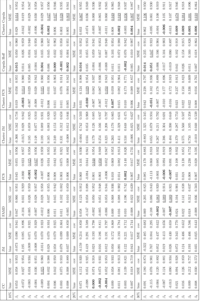
2.3 A comparison of bias, MSE and 95% coverage of coefficients in

random intercept logistic regression model, under eight methods

to handle missing data, with ICC=0.5 and missing rate is 10%,

20% and 30% respectively. . . 41

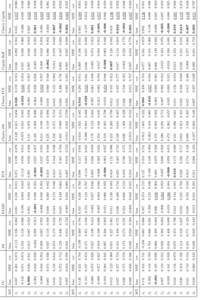
2.4 A comparison of bias, MSE and 95% coverage of coefficients in

random intercept logistic regression model, under eight methods

to handle missing data, with ICC=0.67 and missing rate is 10%,

20% and 30% respectively. . . 42

2.5 Bias, MSE and 95% coverage of the five models of interest under

eight treatments of missing data in the 1000 sub sampled QASC

data sets. . . 46

2.6 Intra-class correlations for variables in the QASC data set . . . . 47

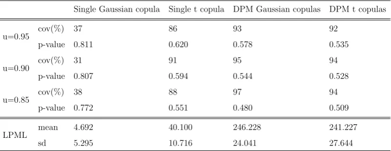
3.1 Coverage and Bayesian p-value of penultimate tail dependence at

quantile level u=0.95, 0.90, 0.85 and the overall measure LPML

by the four competing methods - single Gaussian copula, single t

copula, DPM Gaussian copulas and DPM t copulas. . . 73

(20)

3.3 A comparison of bias, MSE and 95% coverage of the coefficient

estimates under four treatments of missing data - complete case

analysis (CC), fully conditional specification (FCS), single

sian copula (single copula) and Dirichlet process mixture of

Gaus-sian copulas (DPM copula). . . 76

3.5 A comparison of bias, MSE and 95% coverage of the coefficient

estimates in the five models of interest under four treatments of

missing data - complete case analysis (CC), fully conditional

spec-ification with random effects (FCS), single Gaussian copula with

random effects (single copula) and Dirichlet process mixture of

Gaussian copulas with random effects (DPM copula). . . 79

4.1 Comparison of cohort difference in each question by 1) mean

re-sponses in the two cohorts, 2) frequentist p-values from t-test or

χ2-test, 3) our proposed model (GCM Lasso), 4) Gaussian copula

graphical model with G-Wishart prior (BDgraph). The significant

differences are in bold. . . 97

4.2 The conditional association parameters of variables related to high

pain score whose 95% credible intervals did not contain 0. . . 104

4.3 Comparisons of distributions of selected variables between the girls

with predictive scores for endometriosis in the top 10% quantile

and the study population. . . 109

4.4 Coverage rates of the unique parameters in the Ω and Ψ matrices. 111

A.1 Potential scale reduction factors ˆRof the unique elements in Ψ and Γ matrices. . . 122

B.1 A comparison of bias, MSE and 95% coverage of coefficients in

generalized estimating equation, under eight methods to handle

missing data, with ICC=0.5 and missing rate is 10%, 20% and

(21)

LIST OF TABLES 5 B.2 A comparison of bias, MSE and 95% coverage of coefficients in

generalized estimating equation, under eight methods to handle

missing data, with ICC=0.67 and missing rate is 10%, 20% and

30% respectively. . . 127

ran-dom intercept linear model, under eight methods to handle missing

data, with ICC=0.5 and missing rate is 10%, 20% and 30%

respec-tively. . . 128

ran-dom intercept linear model, under eight methods to handle missing

data, with ICC=0.5 and missing rate is 10%, 20% and 30%

(22)

(23)

Chapter 1 Introduction

Missing data are a common occurrence in real data sets, and the direct

appli-cation of standard statistical techniques proposed for complete data sets may

produce invalid statistical inference. Some ad-hoc methods, for example,

com-plete case analysis and available case analysis, might be inadequate to handle

missing data, especially when the missing data are spread over many variables

leading to a dramatic decrease in sample size. In a Bayesian model, missing

val-ues are treated as unknown quantities along with model parameters, and can be

integrated into the statistical analyses. When there are many statistical

analy-ses to be performed perhaps from different parties, an all-in-one approach is to

impute missing values first, so that after imputation complete data analysis can

be performed using standard software. A single imputation of missing values is

inadequate, because the uncertainty in the missing values may result in an

un-derestimate of the standard errors of the quantities being estimated. Therefore

multiple imputation procedure is required for valid inference.

A good imputation method aims to capture the true relationships among

vari-ables. In this thesis, we consider the following statistical challenges when building

an imputation model: 1) dealing with variables of mixed type, including

continu-ous, binary, ordinal and nominal variables; 2) modelling multilevel data sets where

cluster effects are strong; 3) accounting for heterogeneity in the population which

(24)

might be unknown a priori; and 4) the presence of a large number of variables

with strong associations. Our proposed models are all based on the copula model

which is proven to be a powerful tool to analyse multivariate data of mixed-type.

We add variations to the basic Gaussian copula model to accommodate different

features of the data.

The outline of this thesis is as follows. In Chapter 1, we provide background

literature on the general framework of multiple imputation of missing data,

dis-cuss some commonly used imputation models and introduce the two real data

sets used in the thesis.

In Chapter 2 we propose a copula-based method to handle missing values in

multivariate data of mixed-type in multilevel data sets. Building upon the

ex-tended rank likelihood approach and a multinomial probit model, our model is a

latent variable model which is able to capture the relationship among variables of

mixed-type as well as accounting for the clustering structure. We fit the model by

approximating the posterior distribution of the parameters and the missing values

through a Gibbs sampling scheme. We use the multiple imputation procedure to

incorporate the uncertainty due to missing values in the analysis of the data. Our

proposed method is evaluated through simulations using both artificial data and

a real data set from a cluster randomized control trial of acute stroke care

pa-tients, and we compare our proposed imputation model with several conventional

imputation methods.

In Chapter 3, we consider a Bayesian nonparametric approach to imputation

by using an infinite mixture of elliptical copulas induced by a Dirichlet process

mixture to build a flexible copula function. A slice sampling algorithm is used

to sample from the infinite dimensional parameter space. We extend the work

on prior parallel tempering used in finite mixture models to the Dirichlet process

mixture model to overcome the mixing issue in multimodal distributions. Using

simulations, we compare the performance of overall fit and the ability to capture

(25)

1.1. MULTIPLE IMPUTATION OF MISSING DATA 9 model is also applied to the acute stroke data set.

In Chapter 4, motivated from a large population based study of menstrual

dis-order in Australian teenagers, we propose a Gaussian copula model with graphical

lasso prior to identify cohort differences in menstrual characteristics over an 11

year interval and to identify girls with a higher risk of developing endometriosis.

The model includes random effects to account for potential clustering by school,

and we use the extended rank likelihood copula model to handle variables of

mixed-type. The graphical lasso prior shrinks the elements in the precision matrix

of a Gaussian distribution to encourage a sparse graphical structure, where the

level of shrinkage is adaptable from the strength of the conditional associations.

We apply this model to answer some clinical questions of interest, specifically to

analyse the conditional associations among the questions in the questionnaire,

compare cohort differences of menstrual characteristics and to predict the

likeli-hood of developing endometriosis.

In the appendices, we discuss the identifiability issue in our Bayesian latent

models, provide supplementary tables for the model comparisons in Chapter 2,

and attach the sample questionnaire of the menstrual disorder data set.

1.1 Multiple imputation of missing data

1.1.1 Missing data mechanism

To give a principled treatment to the missing data problem, it is important to

dis-tinguish between different missing data mechanisms. Let Y denote the complete

data, with the observed part Yobs and the missing part Ymis, and the sampling

model is p(Y|θ) whereθ denotes the parameter describing the complete data Y. Let Rij be the missing data indicator, where i is the index of units and j is the

index of variables, such that rij = 1 ifYij is observed andrij = 0 ifYij is missing.

According to the factorization by the selection model (Little and Rubin, 2002,

(26)

mecha-nism, where ψ is the parameter in the density function which is distinct from the parameter θ in the sampling model. Rubin (1976) classified the missing data mechanism into the following three categories.

• If the missing data are Missing Completely At Random (MCAR), then

p(R|Y, ψ) = p(R|ψ). That is, the probability of missingness does not depend on the data.

• If the missing data are Missing At Random (MAR), then p(R|Y, ψ) =

p(R|Yobs, ψ). That is, the probability of missingness depends on the

ob-served data only.

• If the missing data are Not Missing At Random (NMAR), thenp(R|Y, ψ) =

p(R|Yobs, Ymis, ψ). That is, the probability of missingness depends on

ob-served data and unobob-served data.

MCAR and MAR are classified as ignorable missing mechanisms, in that

inference about the model parameter θ is only based on the observed data Yobs

through p(θ|Yobs), but not on the missing indicator R and the missing data Ymis.

Therefore no extra effort is needed to model the missing data process p(R|Y, ψ). MCAR assumes the missing data are simple random samples from the complete

data set, whereas MAR assumes missingness depends on the observed data, so

Yobs provides information onYmis. In this thesis, we propose models to handle the

MAR missing data mechanism, which includes MCAR as a special case. However,

the MAR assumption cannot be tested except under artificial simulation settings

because the missing values are unknown. It is a simplifying assumption which can

be made more reasonable by explicit modelling of the missing data mechanism.

Under the Bayesian framework, bothθandYmisare treated as unknown

quan-tities whose joint posterior distribution is p(θ, Ymis|Yobs). That is, conditional on

the observed data, we impute missing values as well as make inference on the

parameters. Simulation based computational methods, like data augmentation,

(27)

1.1. MULTIPLE IMPUTATION OF MISSING DATA 11 values fromp(θ|Y) andp(Ymis|Yobs, θ) is more tractable. Then the pseudorandom

draws of (θ, Ymis) can be treated as coming from the joint posterior distribution,

and the marginal distributions of the variables of interest can be obtained easily

by extracting the relevant quantities from the pseudorandom draws.

1.1.2 Multiple imputation

Multiple Imputation (MI), which was proposed by Rubin (1976), takes every mth

imputed value from the marginal distribution,p(Ymis|Yobs, θ), of the missing values

independently (m needs to be large to ensure independence between consecutive

imputed values) to form M ‘complete’ data sets, and the methods designed for

complete data sets can be used for each imputed ‘complete’ data set. Combining

rules (Rubin, 1987) are applied to estimate from each ‘complete’ data set to

obtain a single inferential result for the quantity of interest. The imputer and

the data analyst can be different individuals, and the analyst may have several

models of interest which are usually different from the imputation models. The

imputation procedure may be carried out by the data collectors or statistical

agencies who have more knowledge of the data set and underlying population to

build sophisticated imputation models and this detailed knowledge is usually not

available to external data analysts. Because of the information non-transparency

between the two parties, MI may suffer from uncongeniality issues (Meng, 1994),

therefore it is advised that the imputation models should take into account the

sampling design and include as many variables as possible.

MI has been an increasingly dominant approach to handle missing data. It is

very flexible in the sense that it allows for the inclusion of any variables that are

potentially related to the missing data to make the MAR assumption more

plau-sible, and the imputation models can be complex to accommodate any features

of the data sets. Furthermore, complete data analyses can be applied directly

using available software without extra modeling or coding efforts.

(28)

scalar quantity of interest, and let q(m) _{be the point estimate of} _Q _{from the} _mth

imputed complete data set, with the associated variance estimate u(m)_{. Then the} point estimate of Q is the mean value of q(m) ₍_m ₌_{₁_{, ..., M}_}₎

¯

Q= 1

M M

X

m=1

q(m). (1.1)

The sampling variance of ¯Qis estimated by combining the within imputation vari-ance ¯U = _M1 PM

m=1u

(m)_{, and the between imputation variance}_B ₌ 1 M−1

PM

m=1(q

(m)₋

¯

Q)2, as follows

T = ¯U + 1 + 1

MB

. (1.2)

The second component of equation (1.2), 1 + _M1B, inflates the variance esti-mate to account for additional uncertainty due to the presence of missing data.

The pivotal statistics T−1/2₍_Q₋_Q_¯_{) follows a} _t _{distribution with degrees of}

freedom ν

T−1/2(Q−Q¯)∼tν, (1.3)

where ν = (M −1) 1 + ₍₁₊_MU¯−1₎_B

2

.

The combining rules for multidimensional estimands are similar to the scalar

quantity and are described in detail in Reiter (2005). In this thesis, we apply

the combining rules to obtain coefficients estimates from generalized linear mixed

effects models and generalized estimating equations.

1.2 Imputation models

Common default methods to handle missing data are complete case analysis and

available case analysis. Although these are easy to implement, they may lead

to loss of information from the incomplete cases and produce biased estimates

when the data are not MCAR. In a data set with a large number of variables,

(29)

1.2. IMPUTATION MODELS 13 all the variables together, there may remain very few complete cases. Available

case analysis, uses complete subsamples to perform different analyses, meaning

the reference population also changes between different analyses leading to

in-compatibility. Other ad-hoc approaches include mean imputation by filling in

the missing values with the mean of the observed values, and last observation

carried forward which uses the last available measurement to fill in the missing

values in longitudinal data. These simple treatments of missing data only make

use of the marginal distribution of the variable, and ignore the relationships

be-tween variables. If the missingness mechanism is not MCAR, the observed data

in other variables can also provide information on the missing data values, and

imputation models should take advantage of this.

Model-based imputation models can be broadly classified into two approaches

in the literature: joint modelling (JM) (Little and Rubin, 2002) and fully

condi-tional specification (FCS) (Raghunathan et al., 2001), among others.

1.2.1 Joint modeling

Simple JM approaches usually assume the multivariate data follow some

para-metric forms, for example, a multivariate Gaussian distribution for continuous

variables. Suppose the variables Y1, ..., Yp follow a p-variate Gaussian

distribu-tion, with mean µ and covariance Γ. Imputing missing values and making

in-ference on the parameters are easy to perform using a Bayesian approach by

sampling from the posterior distribution p(µ,Γ, Ymis|Yobs). A Gibbs sampler is

constructed by iteratively sampling (µ,Γ, Ymis) from the fully conditional

dis-tributions p(µ|Γ, Y), p(Γ|µ, Y) and p(Ymis|µ,Γ, Yobs) respectively. If conjugate

priors are used for the parameters, all the fully conditional distributions have

closed form solutions. Alternatively, the frequentist EM algorithm was designed

for dealing with missing data, to maximize the likelihood function in the presence

of missing data by computing the expected missing values and maximizing the

(30)

of the fact that conditional on the complete data, inference on the parameters is

easier to carry out.

Some variations of the multivariate Gaussian model can be used to better suit

the data sets. For example, a multivariate t distribution enhances robustness.

Some transformations of continuous variables (for example Box-Cox

transforma-tions) are applied to approximate the assumed distribution (Goldstein et al.,

2009), and discrete variables are treated as if they were generated from the

un-derlying continuous variables and then discretized. In many imputation models,

the variables with missing values are first transformed into responses which are

assumed to follow a Gaussian distribution and then regressed against the fully

observed variables. The software packages that implement this approach include

‘norm’ (Schafer and Olsen, 1998) and ‘Amelia’ (Honaker et al., 2011) in R and

‘PROC MI’ in SAS.

Other JM techniques include loglinear models for categorical data which model

the cell probabilities in a contingency table, general location models (Little and

Rubin, 2002) for mixed data which specify a loglinear model for discrete

vari-ables and a Gaussian model for continuous varivari-ables conditional on the discrete

variables, and factorial analysis (Josse and Husson, 2016) which concatenates

standardized continuous variables and discrete variables by indicator variables to

fit a weighted principle component analysis model. Multiple imputation by

loglin-ear models, general location models and factorial analysis have been implemented

in ‘cat’, ‘mix’ and ‘missMDA’ packages in R respectively.

1.2.2 Fully conditional specification

The assumption of the parametric joint distribution of variables is often violated

in real data applications. The Fully Conditional Specification (FCS) approach,

on the other hand, approximates the joint model by a series of univariate response

models. All the models are iterated through by estimating model parameters and

(31)

1.2. IMPUTATION MODELS 15 the FCS in each iteration t are outlined as follows.

• sample θt₁ ∼p(θ1|y1obs, y t−1 2 , ..., yt

−1 p ),

• sample y₁mis,t∼p(ymis

1 |yobs1 , θ1t, y

t−1 2 , ..., yt

−1 p ),

• sample θt

2 ∼p(θ2|y2obs, yt1, ..., yt −1 p ),

• sample y₂mis,t∼p(ymis

2 |yobs2 , θ2t, y1t, ..., yt −1 p ),

.. .

• sample θt

p ∼p(θp|ypobs, yt1, ..., ytp−1),

• sample ymis,t

p ∼p(ypmis|yobsp , θpt, y1t, ..., ypt−1),

where θt

p is the parameter in thepth conditional imputation model at iterationt.

The imputation model for each variable with missing values can be very

flex-ible to accommodate different types and shapes of variables as well as adding

constraints. Generalized linear models (Raghunathan et al., 2001; Van Buuren,

2007) are often used for variables of mixed-type, and tree-based models

(Bur-gette and Reiter, 2010) allow for nonlinear relationships among predictors. The

main criticism of the FCS methods, however, is the lack of theoretical

justi-fication to ensure the conditional distributions for each variable converge to a

target joint distribution, which is guaranteed in JM approaches. FCS has been

implemented by many software packages, for instance, ‘mice’ (Van Buuren and

Groothuis-Oudshoorn, 2010) and ‘mi’ (Su et al., 2011) in R, ‘ice’ in STATA

(Roys-ton et al., 2005) and a SAS-based standalone software ‘IVEware’ (Raghunathan

et al., 2002). The ‘mice’ package is very popular in practice, and the default

method uses predictive mean matching to select a subset of subjects from whom

to sample missing values.

The discussion around the use of FCS and JM is about the correctness of

model specification and the feasibility of implementation. Some practitioners

(32)

joint model for complicated data sets. Several papers have compared JM and

FCS approaches, but there is no clear conclusion under which circumstances

practitioners should favour one over the other. Lee and Carlin (2010) performed

simulations under three missing data mechanisms and their results showed that

JM and FCS produced similar results despite the data not being multivariate

normal. Kropko et al. (2013) not only assessed the accuracy of the coefficients

fitted to models of interest, but also the accuracy of imputed values. Their

study found that FCS imputed more accurately for categorical variables than JM

but the differences were small for continuous variables. Zhao and Yucel (2009)

studied the performance of JM and FCS in multilevel settings, and showed using

simulations that FCS produced less biased estimates than JM, and when the

intraclass correlation is small, more accurate parameter estimates are obtained

from both JM and FCS.

1.2.3 Copula models

1.2.3.1 Basics in copulas

Copula modelling, which is another joint modelling approach, has the potential

to inherit the merits from both JM and FCS, as it provides flexibilities in the

marginal distributions, while ensuring a proper joint distribution at the same

time. In the thesis, we consider copula-based models to impute missing values.

The word ‘copula’ means ‘a link, tie, bond’. In mathematics and statistics,

gener-ally speaking, it means joining together one-dimensional cumulative distribution

functions (CDF) F1, ..., Fp of variables y1, ..., yp to form a joint CDF, F. Each of

the variables is modeled by the marginal distribution Fl(yl) =ul, l = {1, ..., p},

which is uniformly distributed, and the dependence amongu= (u1, ..., up) is

cap-tured by the copula function C. More formally, a copula function C : [0,1]p →

[0,1], is defined as the joint CDF of the uniformly distributed random variables

u1, ..., up, such that C(u1, ..., up) = p(U1 ≤ u1, ..., Up ≤ up). An equivalent but

(33)

1.2. IMPUTATION MODELS 17 Copula models are commonly used for constructing multivariate CDFs, as implied

by the Sklar’s theorem (Sklar, 1959). Sklar’s theorem shows that there always

exists a copula function C, such that F(y1, ..., yp) =C(F1(y1), ..., Fp(yp)), and C

is unique if the random variables yl, l={1, ..., p}, are continuous.

One merit of using a copula model is its invariance property, such that if

T1, ..., Tp are strictly increasing functions, then C is also the copula of the

trans-formed variablesT1(y1), ..., Tp(yp). Also, while Pearson’s correlation measures the

linear relationship between two variables, it is not suitable for quantifying

non-linear relationships. Some rank-based association parameters, such as Kendall’s

tau τ and Spearman’s rho ρ (Embrechts et al., 2002) which describe the

con-cordance between two variables, and tail dependence which describes the

co-movement between extreme values (to be discussed in Chapter 3, Section 3.4.1),

can be computed as functions of the association parameters in copula models.

For example, consider two continuous random variables y1 and y2, and their

corresponding univariate CDFs F1 and F2 respectively. Define the uniformly

distributed random variables as u = F₁−1(y1) and v = F2−1(y2) respectively.

Kendall’s tau τ, Spearman’s rho ρ, lower tail dependence λlw and upper tail

dependence λup can be calculated from a copula function as follows

τ = 4

Z 1

0

Z 1

0

C(u, v)dC(u, v)−1,

ρ= 12

Z 1

0

Z 1

0

C(u, v)dudv−3,

λlw = limt→0+

C(t, t)

t , λup= 2−limt→1−

1−C(t, t)

1−t .

(1.4)

The simplest copula is the independent copula, such that C(u, v) = uv if and only ify1 and y2 are independent. A slightly more complicated class of copulas is the Archimedian copulas including Clayton, Frank and Gumbel copulas. As an

example, the Clayton copula is given by Cα(u, v) = max [u−α+v−α−1]−1/α,0

,

(34)

Clayton copula is asymmetric, in the sense that its upper tail dependence

param-eter is λup = 0, and lower tail dependence parameter is λlw = 2−1/α. Another

class of copulas is the elliptical copulas including Gaussian and t copulas, which

shall be discussed in more detail in Section 2.2 and Section 3.2.2. The

relation-ships between the association parameter α in elliptical copulas with Spearman’s rho and Kendall’s tau are ρ= _π6arcsin(α₂) and τ = 2_πarcsin(α) respectively. Note that both the Gaussian and t copula are symmetric copulas, but the Gaussian

copula is asymptotically independent in its tails, but the t copula has a certain

amount of tail dependence controlled by the degrees of freedom parameter. In the

thesis we only consider elliptical copulas, not only because they allow for

differ-ent pair-wise associations between variables when generalizing to more than two

variables, but also because of their mathematical convenience. Moreover, we also

consider a mixture of copulas in Chapter 4, as a convex combination of copulas

(Nelsen, 2007, Section 3.2.4).

We refer to the book by Nelsen (2007) for a more comprehensive review of

copulas and the paper by Trivedi et al. (2007) for a nice summary.

1.2.3.2 Applications of copula models

There exists in the literature many applications using copulas. To list a few,

Bouy´e et al. (2000) summarized the financial applications including credit scoring,

asset returns modelling and risk measurements; Hu (2006) studied the dependence

patterns across financial markets; and more recently Liu et al. (2017) proposed a

time-varying copula model to study the dependent structure between security and

commodity markets. Extreme value copulas have been considered in actuarial

science, where Cebrian et al. (2003) applied their models to a medical claim

database and Dupuis and Jones (2006) illustrated their approaches to four

risk-related data sets. While copula models have their major applications in finance,

actuarial studies and economics, they have been actively studied in other fields as

(35)

1.2. IMPUTATION MODELS 19 spring seasonal precipitation at Australia’s agro-ecological zones; Yin and Yuan

(2009) used a copula regression in Bayesian adaptive design for finding optimal

dosage in oncology; Valle et al. (2018) extended the work of Wu et al. (2015) by

using an infinite mixture of copula models to study the effect of socioeconomic

factors on the relationship between twins’ cognitive abilities.

1.2.3.3 Copula-based imputation

Copula models have proven to be very powerful for modeling variables of

differ-ent types and shapes, when there is an underlying dependence among them. It

adopts a ‘bottom-up’ strategy where the starting point is the marginal

distribu-tions Fl, which are then glued together by the copula function C. In some other

‘top down’ joint modelling approaches, the marginal distributions are fully

de-termined by their parental joint distribution, however constructing a joint model

whose marginal distributions are suitable for each variable can be a daunting

task, especially when there are a large number of variables of mixed type and

they are skewed or multi-modal. By starting from the marginal distributions we

can accommodate the features of each variable and ensure the imputed data take

proper values in the correct range, which is usually a merit of FCS. In addition,

copula models guarantee the existence of a compatible joint distribution which

is not guaranteed by the FCS approach. The multinomial probit models for

or-dered or unoror-dered categorical data can be treated as a special case of a copula

model, because the underlying latent variables corresponding to each category are

assumed to follow a multivariate Gaussian distribution (Albert and Chib, 1993).

Using the copula model as an imputation engine is relatively new but has

drawn some attention in the literature. Käärik (2006) and Käärik and Käärik

(2009) were among the first authors to consider imputation using a Gaussian

copula model where the missing data pattern was monotone. In their papers, they

imputed missing data due to dropouts in longitudinal data sets, where a monotone

(36)

dependencies for the correlation matrix were considered. Lascio (2015) found

that copula based imputation from the Archimedian family compared favourably

with nearest neighbour donor imputation and regression imputation by the EM

algorithm. Hollenbach et al. (2014) compared the performance of imputation

by the copula model using the extended rank likelihood approach (Hoff, 2007)

(to be discussed in Section 2.2) with JM (as implemented in ‘Amelia’ package

in R) and FCS (as implemented in ‘mice’ package in R) and concluded that the

copula imputation approach outperformed the other two approaches in terms

of a slightly smaller bias, higher coverage rate and narrower confidence interval

estimates. The improvement was more pronounced when the missing data were

not normally distributed. They implemented the imputation using the R package

‘sbgcop’ (Hoff, 2018), which has the option to impute missing data under the

MAR assumption. Shen and Weissfeld (2006) considered the NMAR scenario

by building a joint model for the outcome variables and the associated missing

data indicators, and they claimed that it could be used to eliminate the potential

bias caused by the non-ignorable missingness. Generalized estimating equations

(GEE) were used to estimate the marginal distributions of the missing indicators

given the observed data, and then the parameters in the Gaussian copula model

and the marginal distributions of the outcome variables were estimated.

1.3 Application data sets

In this thesis, we propose copula-based models to impute missing data and the

models are evaluated on two clinical data sets as described below - the Quality

in Acute Stroke Care (QASC) study (Middleton et al., 2011), and the survey of

Menstrual Disorder of Teenagers (MDOT) (Parker et al., 2010). Because of the

sensitivity and confidential nature of these data, we would not provide public

access to the data sets. The R code to reproduce the simulation results will be

(37)

1.3. APPLICATION DATA SETS 21

1.3.1 Quality in Acute Stroke Care (QASC) study

The QASC study was a randomized control trial conducted in 2005-2007 which

implemented a multidisciplinary intervention to manage fever, hyperglycaemia

and swallowing dysfunction in acute stroke patients. This study was one of the

largest rigorously evaluated clinical trials which showed that organized stroke

unit care significantly reduced death and disability among stroke patients. There

were 19 acute stroke units in New South Wales, Australia that participated in

the study, and they were randomly assigned to an intervention group (10 units)

or a control group (9 units). A pre-intervention and a post-intervention cohort of

patients were recruited, their demographic variables were obtained, and process

of care variables and health outcome variables were recorded. The numbers of

patients in the two cohorts were 595 and 885 respectively. The variables were

mixed-type including continuous, ordinal and nominal variables, the data

struc-ture was multilevel where patients were nested within hospitals and almost all the

15 variables contained missing values ranging from 10% to 16%, leading to 75%

complete cases in the study population. The researchers were primarily interested

to see if there were differences between treatment and control groups in health

outcome variables. Our proposed imputation models in Chapter 2 and Chapter

3 were applied to the QASC data set.

1.3.2 Menstrual Disorder of Teenagers (MDOT) study

The Menstrual Disorder of Teenagers (MDOT) survey (Parker et al., 2010) was

conducted in 2005 and 2016 to collect data on the menstrual patterns of teenage

girls. Both surveys were conducted in the Australian Capital Territory (ACT)

us-ing the same questionnaire. The two cohorts of participants were 15-19 years old

teenage girls from 4 senior high schools in 2005, and 3 senior high schools in 2016.

The participating schools were selected based on their number of enrollments and

were located across the ACT region. Consent forms were signed by the parents

(38)

was maximized by the careful design of the questionnaire, getting support from

participating schools, and allocating time to fill in the questionnaires during class.

The consistency of the data from the two cohorts was guaranteed by using the

same questionnaire and following the same data collection procedure from 2005

in 2016. There were more than 100 questions in the questionniare, covering

per-sonal information, typical menstruation characteristics, menstrual symptoms, life

interference, menstrual experiences, and knowledge and diagnosis of some

men-struation diseases. Due to the large number of questions in the questionnaire,

less than 2% of participating girls provided complete answers to every question.

Using the MDOT data set, a range of clinical questions can be asked, such as,

which menstrual characteristics are changing over time, and can the MDOT

ques-tionnaire identify girls with a higher risk of developing endometriosis. We will

investigate some questions of particular interest in Chapter 4.

These two data sets serve as our motivating examples, and we believe that

our developed methods can be adapted to other data sets with similar structure,

for example, a three-layer hierarchical model. Our proposed models can not only

be used as imputation engines for missing data, but more generally provide an

(39)

Chapter 2 Copula based imputation model

for multilevel data sets

2.1 Introduction

Multivariate analysis often involves understanding the relationships among

vari-ables of different types. Our motivating data set is from a randomized control

trial - the Quality in Acute Stroke Care (QASC) study (Middleton et al., 2011),

which implemented a multidisciplinary intervention to manage fever,

hypergly-caemia and swallowing dysfunction in acute stroke patients. Most of the variables

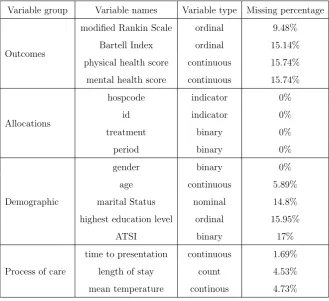
in this multilevel data set contained missing values, and they were of mixed type

(Table 2.1). In the ‘variable group’ column, ‘outcomes’ refers to the primary

outcomes that assess the patients’ health status, and ‘process of care’ refers to

the secondary outcomes during patients’ stay in hospital. ‘Allocations’ tracks

the patients’ assignment to cohorts, treatment groups and hospitals. Ignoring all

the patients with missing values is a commonly used approach to handle missing

data but may lead to biased estimates and reduced statistical power (Van Buuren

et al., 2011). The smaller sample size decreases the power to detect significant

treatment effects, and this is especially serious in multilevel data sets due to the

potential for positive dependence among units within the same cluster, such as

(40)

patients in a hospital. In this chapter, we use the multiple imputation (MI)

ap-proach by filling in missing values from our proposed imputation models, and

then perform statistical analyses on the imputed complete data sets.

Variable group Variable names Variable type Missing percentage

Outcomes

modified Rankin Scale ordinal 9.48%

Bartell Index ordinal 15.14%

physical health score continuous 15.74%

mental health score continuous 15.74%

Allocations

hospcode indicator 0%

id indicator 0%

treatment binary 0%

period binary 0%

Demographic

gender binary 0%

age continuous 5.89%

marital Status nominal 14.8%

highest education level ordinal 15.95%

ATSI binary 17%

Process of care

time to presentation continuous 1.69%

length of stay count 4.53%

[image:40.595.113.443.177.478.2]

mean temperature continous 4.73%

Table 2.1: Summary of variables in the QASC data set

Current imputation models to handle missing data are potentially inadequate

to apply to the QASC study which is complicated by the clustering effect of

patients within acute stroke units and the mix of variable types (Goldstein et al.,

2009). Hoff (2007) proposed using a semiparametric copula model based on the

extended rank likelihood to analyse multivariate data of mixed types. We extend

the work of Hoff (2007) by adding random effects to introduce correlation among

individuals within clusters, and allow for unordered nominal variables through a

multinomial probit model.

The structure of this chapter is as follows. In Section 2.2 we review

(41)

2.2. THE EXTENDED RANK LIKELIHOOD OF GAUSSIAN COPULA 25 models as discussed in Hoff (2007). In Section 2.3 we describe our proposed

im-putation model for multilevel data of mixed type by fusing the Gaussian copula

model and the multinomial probit model, and we outline our computational

algo-rithm using Gibbs sampling. In Section 2.4, we present and discuss the results of

two sets of simulations comparing our proposed method to seven existing

meth-ods, and implement a real data analysis. Section 2.5 provides concluding remarks

and discussions. The identifiability issues and convergence checks of our proposed

model are discussed Appendix A, and further simulation results are presented in

Appendix B.

2.2 The extended rank likelihood of Gaussian

copula

Recall in a copula model, the joint distribution of variables y1, ..., yp is

decom-posed into the marginal distributions F1, ..., Fp and a copula function C, such

that F(y1, ..., yp) = C(F1(y1), ..., Fp(yp)). The parameters are those that

char-acterize the marginal distributions Fl and the copula function C. Pitt et al.

(2006) developed a fully Bayesian estimation procedure to model the joint

distri-bution of both sources of parameters. However, specifying each of the marginal

distributions is labour intensive and variables in real data sets may not be

accu-rately represented without a large number of parameters. Some authors suggested

transforming the variables using the empirical distribution ˆFl to obtain pseudo

data (Genest et al., 1995) and avoid the parametric estimation of marginal

dis-tributions. However, this only applies to continuous variables. As noted by Hoff

(2007), ‘the pseudo-data estimators of copula parameters will be problematic for

discrete data because transformation of such data do not really change the data

distribution, they just change the sample space’. To link the discrete variables

with continuous latent variables, Hoff (2007) provided a simple way of analysing

(42)

or-dered categorical variables), via the extended rank likelihood. This makes use

of the fact that the order of the underlying latent variable is consistent with the

observed data, and inference about the association parameters can be drawn from

the ‘rank-based’ latent variables through a simple parametric form.

Among a variety of copulas, we focus on the Gaussian copula in this

chap-ter which specifies a joint multivariate Gaussian distribution on the latent

vari-ables, rather than assuming a Gaussian distribution on the data y directly. The Gaussian copula only applies to continuous data, but we will see shortly how

this restriction is relaxed when applied to the variables on the latent scale. Let

l = {1, ..., p} denote the index of the lth _{random variable.} _{Then the} _lth

la-tent variable is zl = Φ−1(ul), where ul = Fl(yl). That is, C(u1, ..., up|Γ) =

Φp(Φ−1(u1), ...,Φ−1(up)|Γ) = Φp(z1, ..., zp|Γ), where Φp(·|Γ) is the cumulative

dis-tribution function of the p-variate normal distribution, with mean zero and cor-relation matrix Γ.

In the rank-based extended rank likelihood approach for ordered variables by

Hoff (2007), when estimating the correlation matrix Γ, there is no need to specify

the marginal distributions Fl. The idea is that since we know Φ−1(F(·)) is a

monotone transformation, the ordering of the datayprovides partial information about what z should be, that is, yi1l < yi2l implies zi1l < zi2l. Suppose we have

in total N observations, n = {1, ..., N}. Observing y = (y1, ..., yN) tells us that z = (z1, ..., zN) must lie in the set:

z ∈ _RN×p _: _max_{_z

hl : yhl < ynl} < znl < min{zhl :yhl > ynl} . Let ‘D’ denote the set of all possiblez which is consistent

with the ordering of y. Then the event ‘z ∈ D’ can be treated as the observed event upon which inference of Γ is made. The full likelihood can be decomposed

as

p(y|Γ, F1, ..., Fp) = p(z∈D, y|Γ, F1, ..., Fp)

=p(z∈D|Γ)×p(y|z ∈D,Γ, F1, ..., Fp).

(2.1)

Based on partial sufficiency, Hoff (2007) showed that inference for Γ is based on

(43)

2.2. THE EXTENDED RANK LIKELIHOOD OF GAUSSIAN COPULA 27 for discrete variables. However, this approach means that we do not need to

estimate the potentially complicated marginal distribution functions, suggesting

that the rank likelihood provides a more general and flexible framework for joint

modelling.

As an illustration, we show some basics of the extended rank likelihood of

Gaussian copula via a toy example. We consider an ordinal variable y1 =

(y11, y12, y13, y14, y15) = (1,3,3,2,NA), where ‘NA’ stands for a missing value, and a continuous variabley2 = (y21, y22, y23, y24, y25) = (11.22,31.59,32.92,12.11,62.30). We would like to see the association between these two variables. The values

of z must satisfy the ordering of y, for example, z1 = (z11, z12, z13, z14, z15) = (−1.10,−0.09,−0.12,−0.27,1.94), and z2 = (z21, z22, z23, z24, z25) =

(−0.67,0.13,0.34,−0.51,1.59). Note that (z1, z2) ∼ N (0,0),

1 γ12

γ12 1

. In the

next iteration when updating z11, we sample from the truncated normal distri-bution N(γ12z21,1− γ122 )δ(lb,ub), where the lower bound and upper bound are lb = −∞ and ub = −0.27. This is because y11 is the smallest value in y1 so the lower bound is negative infinity, and y14 is the smallest value in y1 which is bigger than y11 and corresponding latent variable value z14 = −0.27. Similarly, we update z14 from the truncated normal distribution N(γ12z24,1−γ122 )δ(lb,ub),

where the lower bound and upper bound are lb = −1.1 and ub =−0.12. When

y15 is missing, the neighboring points are undefined, therefore it is sampled from

N(γ12z25,1−γ122 ) without truncations.

The extended rank likelihood has already been applied to other closely related

models, for example, a general Bayesian Gaussian copula factor model proposed

by Murray et al. (2013) and a bifactor model considered by Gruhl et al. (2013), can

be treated as imposing a special structure on the correlation matrix of a Gaussian

copula. Dobra et al. (2011) and Mohammadi et al. (2017) used the extended rank

likelihood Gaussian copula to make inference on a graphical model, which will be

(44)

2.3 Copula model for mixed type variables

2.3.1 Model specification

We extend Hoff’s work by adding random effects to the Gaussian copula model

at the latent variables level, to account for groupings/clustering in the observed

data. Formally we assume

zij|bi1 ∼Np(bi1,Γ1), bi1 ∼Np(0,Ψ1), (2.2)

where i = {1, ..., m} is the group index, j = {1, ..., ni} is the individual index within group i, and Γ1 and Ψ1 are variance-covariance matrices for zij and bi1 respectively. Both zij and bi1 are vectors of lengthp, because we are considering

l ={1, ..., p} variables jointly. In this model, the parameters that need to be es-timated are in (Γ1,Ψ1), which can be thought of as splitting the total correlation into two parts, the variability within groups and the variability between groups.

However, like any model that relies on the ordering of the data but not their

mag-nitude, model (2.2) suffers from an identifiability problem without constraints on

Γ1 and Ψ1. The extended rank likelihood contains only the information about

the relative ordering of z but no information about their location and scale. To solve the identifiability problem of scale based on our specific model formulation,

we fix the sum of Γ1 and Ψ1 to be a correlation matrix. Because the marginal

distributions of z have means equal to 0, there is no identifiability issue for loca-tion. The intra-class correlation (ICC) for each variable on the latent scale can

be read off from the diagonal elements in the Ψ1 matrix as ICCl =ψl2, where ψl2

are the elements along the diagonal of Ψ1. Further justifications of choosing the

constraint for solving the identifiability problem are contained in Appendix A.

Notice that the extended rank likelihood described above only applies to

con-tinuous and ordinal variables, since it makes no sense to consider meaningful

numeric values for nominal variables (categorical variables without ordering). To

include nominal variables in the copula model as well, we consider a multinomial

(45)

2.3. COPULA MODEL FOR MIXED TYPE VARIABLES 29 The idea is to relate a nominal variable to a vector of latent variables which can

be thought of as the unnormalized probabilities of choosing each of the categories.

Suppose a single nominal variabley hasK categories, and we defineK−1 latent variables for uniti as wi = (wi1, ..., wi,K−1) which follow a multivariate Gaussian distribution. The intercept term β vector is used to represent the relative differ-ences between each category 1, ..., K−1 compared with the baseline category. To add a second level to the hierarchy, again we have the random effects bi2 in the model

yij =

  

 

k if wijk > wijk0 and w_ijk >0, for k0 6=k

K if wijk<0, for all k ={1, ..., K−1},

wij =β+bi2+ij,

bi2 ∼NK−1(0,Ψ2), ij ∼NK−1(0,Γ2).

(2.3)

The rule of deciding the category is a mapping from the latent variables vector

to the observed category. The category k = {1, ..., K −1} is observed if the

kth element of the vector wi is the largest and greater than 0; the last

cate-gory K is observed if the largest element in wi is smaller than 0. Because we

do not have substantial interest in the association between levels in a nominal

variable (Goldstein et al., 2009), we fix Γ2 to be a diagonal matrix such that

Γ2 =





γ2

1 0

. ._.

0 γ2

K−1



, and for identifiability reasons similar to the extended rank

likelihood we fix the sum of Γ2 and Ψ2 to be a correlation matrix.

To provide a unified framework of the multivariate analysis of mixed variable

types, we combine model (2.2) for variables with ordering and model (2.3) for

(46)

zij|bi1 ∼Np(bi1,Γ1), wij ∼NK−1(β+bi2,Γ2),

bi = (bi1, bi2)∼Np+K−1(0p+K−1,Ψ),Ψ =





Ψ1 Ψ12

Ψ21 Ψ2



,

(zij, wij)|bi ∼Np+K−1((0p, β) +bi,Γ),Γ =





Γ1 0

0 Γ2



.

(2.4)

The combined random effectsbiis a vector of lengthp+K−1, which is composed

of the random effects bi1 for the ordered variables and bi2 for the nominal vari-able. The correlations between variables y1, ..., yp and yp+1 are modeled through the off-diagonal matrices Ψ12(Ψ21). This model assumes that conditional on the

random effects, the ordered variables and the nominal variable are independent,

but marginally they are not because the random effects are correlated. In this

model, all the parameters are identifiable (see the Appendix A for further

discus-sion).

2.3.2 A Gibbs sampler

A Gibbs sampling scheme is constructed to examine the joint posterior

distri-bution p(β,Ψ,Γ, b, z, w, ymis|yobs) where the unknown quantities in model (2.4)

are the parameters (β,Ψ,Γ), the latent variables (b, z, w) and the missing data

ymis. To impose the sum constraint such that Ψ + Γ is a correlation matrix, we

follow the idea in Hoff (2007) of employing a parameter expansion approach (Liu

and Wu, 1999). Specifically, we put Inverse Wishart priors on ˜Ψ and ˜Γ1, and

inverse gamma priors on the diagonal elements ˜γ₁2, ...,γ˜_K2₋₁ in ˜Γ2. The parame-ters with tilde correspond to the parameparame-ters in the augmented model which are

sampled directly in the Gibbs sampler and then they are scaled back to the ones

in the original model (2.4). Then the full conditional distributions of ˜Ψ, ˜Γ1 and

˜

(47)

2.3. COPULA MODEL FOR MIXED TYPE VARIABLES 31 follows

β ∼N(µβ,Σβ),

˜

Γ1 ∼Inv Wishart(ν1,Λ1), ˜

γ₁2, ...,˜γ_K2₋₁ i.i.d.∼ Inv gamma(η, τ),

˜

Ψ∼Inv Wishart(ν2,Λ2).

(2.5)

In our simulations, the hyperparameters are chosen to be weakly informative,

such that µβ = 0K−1, Σβ = IK−1, ν1 = p+ 1,Λ1 = Ip, η = τ = 0.001, ν2 =

p+K, Λ2 = Ip+K−1. Under these priors, it is straightforward to derive the full conditional distributions

1. β ∼N (Σ−_β1+NΓ−₂1)−1_(Σ−1

β µβ+Γ−21

Pm

i=1

Pni

j=1(wij−bi2)),(Σ−β1+NΓ

−1

2 )

−1

;

2. bi ∼N (Ψ−1+niΓ−1)−1Γ−1

Pni

i=1((zi, wi)−(0p, β)),(Ψ−1+niΓ−1)−1

;

3. ˜Γ1 ∼Inv Wishart ν1+N,Λ1+Pm_i₌₁P_jn₌₁i (zij −bi1)T(zij −bi1)

;

4. ˜γ2

k ∼Inv gamma η+

N

2, τ +

1 2

Pm

i=1

Pni

j=1(wijk−βk−bi2k)2

;

5. ˜Ψ∼Inv Wishart(ν2+m,Λ2+Pm_i₌₁bTi bi);

6. Impose the marginal correlation constraint by rescaling ˜Ψ and ˜Γ:

˜ Γ2 =





˜ γ2

1 0

. ._.

0 ˜γ2

K−1



,Γ =˜

˜

Γ1 0

0 Γ˜2

,

Γ[g,h]= ˜Γ[g,h]/

q

(˜Γ[g,g]+ ˜Ψ[g,g])(˜Γ[h,h]+ ˜Ψ[h,h]), Ψ[g,h] = ˜Ψ[g,h]/

q

(˜Γ[g,g]+ ˜Ψ[g,g])(˜Γ[h,h]+ ˜Ψ[h,h]), g, h={1, ..., p+K−1}.

7. zijk ∼N b1ik+ Γ1k−kΓ1−−1k−k(zij−k−bi1−k),Γ1kk−Γ1k−kΓ−1−1k−kΓ1−kk

.

Updating the latent variablezis achieved by sampling from truncated Gaus-sian distributions, where the lower and upper bounds for each single entry

zijl are determined by: lb = max(zhl :yhl < yijl) and ub = min(zhj : yhj > yijl) respectively, and h is the index that searches over all the rows in the lth _{variable. For example, the lower bound for} _z

(48)

of the latent variable z in the lth _{column whose corresponding} _y _{is smaller}

than yijl and the upper bound can be defined accordingly. When there are

missing values in (y1, ..., yp), the lower and upper bounds inz are undefined,

and we sample z from the Gaussian distributions without truncations.

8. Sample wij from the proposal distribution N β+b2i,Γ2

.

Updating the latent variable w is achieved by sampling from multivariate

Gaussian distributions under the constraint of the observed category by an

acceptance and rejection algorithm (Albert and Chib, 1993). Specifically,

we sample a w vector from the multivariate Gaussian distribution and

ac-cept this draw if and only if the maximum element ofw occurs at the place of the observed category and is greater than 0, or all the elements in ware

smaller than 0 and we observe the reference category K. We continue to

sample w until a draw is accepted. When there are missing values in yp+1 so the observed categories do not exist, we sample w from the multivariate Gaussian distributions with no rejections.

9. Impute missing values.

Ordered variables are imputed from z by the monotone transformation

yijl = ˆFl−1[Φ(zijl)], l={1, ..., p}, (2.6)

where ˆFl is the univariate empirical distribution function of variable yl in

each scan of the MCMC. The empirical CDFs from the current iteration are

constructed using both the observed and imputed missing values from the

previous MCMC scan. Notice that by using the empirical CDFs we may

underestimate the uncertainty in the marginal distributions, however this

approach is easy to implement and guarantees that the imputed values are in

the proper range as the observed data. An alternative solution of imputing

missing values from the latent variables could be purely based on the rank

of the pairs z and y, as discussed in Hoff (2007). Specifically, we sortz and

(49)

2.4. SIMULATION STUDIES 33 is between two neighbours zlb and zub, then the missing y is imputed as a

number between ylb and yub corresponding to zlb and zub respectively. The

nominal variables are imputed by choosing the category corresponding to

the largest element in w if it is greater than 0, and choosing the reference

category if the largest element in w is smaller than 0. Simulations (not

presented in the thesis) showed that there was not much difference between

these two approaches in terms of imputation accuracy and the ability to

estimate parameters in some models of interest, therefore we used the first

approach by empirical CDF in the subsequent sections.

2.4 Simulation studies

We evaluated the performance of the proposed model through two simulation

studies: (i) simulated artificial data with missing values and (ii) the QASC data

set with randomly deleted records. The simulation settings to generate the

mul-tilevel data of mixed type with the MAR missing records will be explained in

subsequent subsections. We compared our proposed imputation model with seven

other approaches to treat missing data.

2.4.1 Simulation based on artificial data

We generated 1000 complete multilevel data sets with correlated variables of

different types, and then deleted some entries under the MAR assumption. The

total number of clusters in each data set was 20 (i = {1, ...,20}), the cluster size was 50 (j = {1, ...,50}), and the five variables y1, y2, y3, y4, y5 had Gamma, binary, nominal, ordinal, and normal distributions respectively, and y1, y4 and

y5 had clustering effects. The variable y1 was generated first, and we assumed all the subsequent variables were generated depending on the previous ones, to

introduce correlations among variables.

(50)

ef-fects. Denote z1ij the latent variable for the jth unit within cluster i

of variable y1, and y1ij is the associated observed data. We first

gener-ated the latent variable z1ij ∼ N(b1i,1), b1i ∼ N(0, ρ), and then obtained y1ij = F−1( ˜Φ(z1ij)), where F was the CDF of a Gamma distribution with

shape=1 and rate=2, and ˜Φ was the CDF of a Normal distribution with

mean=1 and variance=1+ρ.

• The binary variable y2 was generated by logit(µ2) = y1, where µ2 was the probability that y2 equaled 1.

• The nominal variable y3 had 4 categories and was generated by a

multino-mial probit model, so that 3 latent variables were needed: z3 = (z31, z32, z33)∼

N((y1, y2)B, C), where B was a randomly generated coefficient matrix of dimension 2×3 andC was a correlation matrix of dimension 3×3. The cat-egory iny3was chosen to bek(for k=1,2,3) ifz3kwas the largest component

and was greater than 0; and was chosen to be 4 if max(z3)<0.

• The clustered ordinal variable y4 was first generated by the latent variables

z4ij ∼ N(b4i+ (y1, y2, y3)β4,1), where b4i ∼ N(0, ρ), and β4 is a vector of length 5, corresponding to y1, y2 and 3 categories in y3. Three thresholds were used to determine four levels of y4, they were the 20%, 30%, and 50% quantiles of z4.

• The normally distributed variabley5was generated from a random intercept model,y5ij ∼(b5i+ (y1, y2, y3, y4)β5,1), whereb5i ∼N(0, ρ), andβ5 a vector of length 8, corresponding to the coefficients for y1, y2, 3 categories in y3 and 3 categories in y4.

To create missing data under the MAR assumption, we assumedy5 was

com-pletely observed and that the probabilities of missingness in yl (l = {1, ...,4})

depended ony5. Specifically, letpmis,hl be the probability that observation hwas

Recent developments of copula based models to handle missing data of mixed type in multivariate analysis