Traffic Flow Forecasting Based on Combination of Multidimensional Scaling
and SVM
Zhanquan Sun
a, Geoffrey Fox
ba. Key Laboratory for Computer Network of Shandong Province, Shandong Computer Science Center (19 Keyuan Road, Jinan, Shandong, 250014, China, [email protected])
b. School of Informatics and Computing, Pervasive Technology Institute, Indiana University Bloomington (2719 E 10th St
,
Bloomington, Indiana, 47408, USA, [email protected])Abstract: Traffic flow forecasting is a popular research topic of Intelligent Transportation Systems (ITS). With the development of information technology, lots of history electronic traffic flow data are collected. How to take full use of the history traffic flow data to improve the traffic flow forecasting precision is an important issue. More history data are considered, more computation cost should be taken. In traffic flow forecasting, many traffic parameters can be chosen to forecast traffic flow. Traffic flow forecasting is a real-time problem, how to improve the computation speed is a very important problem. Feature extraction is an efficient means to improve computation speed. Some feature extraction methods have been proposed, such as PCA, SOM network, and Multidimensional Scaling (MDS) and so on. But PCA can only measure the linear correlation between variables. The computation cost of SOM network is very expensive. In this paper, MDS is used to decrease the dimension of traffic parameters, interpolation MDS is used to increase computation speed. It is combined with nonlinear regression Support Vector Machines (SVM) to forecast traffic flow. The efficiency of the method is illustrated through analyzing the traffic data of Jinan urban transportation.
Keywords: Intelligent transportation; Traffic flow forecasting, Multidimensional Scaling; SVM; Interpolation
1. Introduction
Short-time traffic flow forecasting is a popular research topic of Intelligent Transportation Systems (ITS). Correct traffic flow forecasting is the precondition of real-time traffic signal control, traffic assignment, route guidance, automatic guidance, and accident detection. The study of traffic flow forecasting is very significant in ITS. Many scholars have been studying on the topic and many forecasting models have been developed. Commonly used methods include average method, ARMA, linear regression, nonparametric regression, and neural networks [1-3]. The forecasting precisions of these methods usually can’t meet with the practical requirement. Support Vector Machines (SVM) is proposed by V. Vapnik in 1995[4]. It is a network model that is based on the principle of structure risk minimization and VC dimension theory. It can resolve small sample, nonlinear, high dimension, and local minimum problems efficiently [5]. SVM is mainly used to resolve classification and regression problems. Nonlinear regression SVM has been used to forecast traffic flow and obtained good results [6].
In practical, there are many parameters are available for the traffic flow forecasting. Many forecasting methods are real-time. Too many input parameters will decrease the real-time performance. In current traffic flowing forecasting research, mostly concentrate on short term history traffic flow data. Lots of history data are not taken into consideration because the computation cost is expensive. For taking full use of history traffic flow data and improving the computation speed, feature
extraction is an efficient means. It can decrease the dimension of input and decrease the computation cost efficiently. Many feature extraction methods have been proposed, such as Principal Component Analysis (PCA), Self Organization Map (SOM) network, and so on[7-8]. Multidimentional Scaling (MDS) is a kind of Graphical representations method of multivariate data[9]. It is widely used in research and applications of many disciplines. The method is based on techniques of representing a set of observations by a set of points in a low-dimensional real (usually) Euclidean vector space, so that observations that are similar to one another are represented by points that are close together. It is a nonlinear dimension reduction method. But the computation complexity is O(n^2) and memory requirement is O(n^2). With the increase of sample size, the computation cost of MDS increase sharply. For improving the computation speed, interpolation MDS are introduced in reference [10]. It is used to extract feature from large scale traffic flow data. Nonlinear SVM is used to forecast traffic flow.
The following of the paper is organized as follows. Interpolation MDS method is introduced in part 2. Nonlinear SVM is introduced in part 3. Traffic flow forecasting procedure based on MDS and nonlinear SVM is introduced in part 4. A practical example is analyzed with the proposed model in part 5. At last some conclusions are summarized.
2. Interpolation MDS
MDS is a non-linear optimization approach constructing a lower dimensional mapping of high dimensional data with respect to the given proximity information based on objective functions. It is an efficient feature extraction method. The method can be described as follows.
Given a collection of n objects D =
{x1, x2,⋯, xn}, xi∈RN(i = 1,2,⋯, n) on which a
distance function is defined asδi,j, the pairwise distance matrix of the n objects can be denoted by
∆≔ �
δ1,1 δ1,2
δ2,1 δ2,2 ⋯
δ1,n
δ2,n
⋮ ⋱ ⋮
δn,1 δn,2 ⋯ δn,n
�
whereδi,j is the distance between xi and xj. Euclidean distance is often adopted.
The goal of MDS is, given Δ, to find n vectors
p1,⋯, pn∈RL(L≤N) to minimization the STRESS or
SSTRESS. The definition of STRESS and SSTRESS are as follows.
σ(P) =∑i<jwi,j�di,j(P)− δi,j�2 (1)
σ2(P) =∑ w
i,j�(di,j(P))2− δi2,j�2
i<j (2)
where 1≤i < j≤n, 𝑤𝑤𝑖𝑖,𝑗𝑗 is a weight value (𝑤𝑤𝑖𝑖,𝑗𝑗> 0),
𝑑𝑑𝑖𝑖,𝑗𝑗(𝑃𝑃) is a Euclidean distance between mapping results
of 𝒑𝒑𝑖𝑖 and 𝒑𝒑𝑗𝑗. It may be a metric or arbitrary distance function. In other words, MDS attempts to find an embedding from the 𝑛𝑛 objects into 𝑅𝑅𝐿𝐿 such that distances are preserved.
2.2 Interpolation Multidimensional Scaling
One of the main limitations of most MDS applications is that it requires 𝑂𝑂(𝑛𝑛2) memory as well as O(n2) computation. It is difficult to process MDS with large scale data set because of the limitation of memory limitation. Interpolation is a suitable solution for large scale MDS problems. The process can be summarized as follows.
Given n samples data 𝐷𝐷= {𝒙𝒙1,𝒙𝒙2,⋯,𝒙𝒙𝑛𝑛},𝒙𝒙𝑖𝑖∈
𝑅𝑅𝑁𝑁(𝑖𝑖= 1,2,⋯,𝑛𝑛) in N dimension space, m samples
𝐷𝐷𝑠𝑠𝑠𝑠𝑠𝑠= {𝒙𝒙1,𝒙𝒙2,⋯,𝒙𝒙𝑚𝑚}, are selected to be mapped into
L dimension space 𝑃𝑃𝑠𝑠𝑠𝑠𝑠𝑠 = {𝒑𝒑1,𝒑𝒑2,⋯,𝒑𝒑𝑚𝑚} with MDS. The other samples 𝐷𝐷𝑟𝑟𝑠𝑠𝑠𝑠𝑟𝑟= {𝒙𝒙1,𝒙𝒙2,⋯,𝒙𝒙𝑛𝑛−𝑚𝑚}, will be mapped into L dimension space 𝑃𝑃𝑟𝑟𝑠𝑠𝑠𝑠𝑟𝑟=
{𝒑𝒑1,𝒑𝒑2,⋯,𝒑𝒑𝑛𝑛−𝑚𝑚} with interpolation method. The
computation cost and memory of interpolation MDS is only 𝑂𝑂(𝑛𝑛) . It can improve the computing speed markedly.
Select one sample data 𝒙𝒙 ∈ 𝐷𝐷𝑟𝑟𝑠𝑠𝑠𝑠𝑟𝑟 , calculate the distance 𝛿𝛿𝑖𝑖𝑖𝑖 between the sample data 𝒙𝒙 and the pre-mapped samples 𝒙𝒙𝒊𝒊∈ 𝐷𝐷𝑠𝑠𝑠𝑠𝑠𝑠(𝑖𝑖= 1,2,⋯,𝑚𝑚). Select the 𝑘𝑘 nearest neighbors 𝑄𝑄= {𝑞𝑞1,𝑞𝑞2,⋯,𝑞𝑞𝑘𝑘}, where 𝒒𝒒𝑖𝑖∈ 𝐷𝐷𝑠𝑠𝑠𝑠𝑠𝑠, who have the minimum distance values.
After data set 𝑄𝑄 being selected, the mapped value of the input sample is calculated through minimizing the following equations as similar as normal MDS problem with 𝑘𝑘+ 1 points.
𝜎𝜎(𝑋𝑋) =∑ �𝑑𝑑𝑖𝑖<𝑗𝑗 𝑖𝑖,𝑗𝑗(𝑃𝑃)− 𝜹𝜹𝒊𝒊,𝒋𝒋�2=𝐶𝐶+∑𝑘𝑘𝑖𝑖=1𝑑𝑑𝑖𝑖𝑖𝑖2 −
2∑𝑘𝑘𝑖𝑖=1𝑑𝑑𝑖𝑖𝑖𝑖𝛿𝛿𝑖𝑖𝑖𝑖 (3)
In the optimization problems, only the position of the mapping position of input sample is variable. According to reference [10], the solution to the optimization problem can be obtained as
𝑥𝑥[𝑟𝑟]=𝒑𝒑�+1
𝑘𝑘∑ 𝛿𝛿𝑖𝑖𝑖𝑖
𝑑𝑑𝑖𝑖𝑖𝑖�𝑥𝑥
[𝑟𝑟−1]− 𝒑𝒑
𝑖𝑖� 𝑘𝑘
𝑖𝑖=1 (4)
where 𝑑𝑑𝑖𝑖𝑖𝑖=�𝒑𝒑𝑖𝑖− 𝑥𝑥[𝑟𝑟−1]� and 𝒑𝒑� is the average of k pre-mapped results. The equation can be solved through iteration. The iteration will stop when the difference between two iterations is less than the prescribed threshold values. The difference between two iterations is denoted by
𝛿𝛿=(�𝑖𝑖[�𝑖𝑖𝑡𝑡]−𝑖𝑖[𝑡𝑡−1[𝑡𝑡−1]�]�) (5)
3. Support Vector Machines
SVM first maps the input points into a high-dimensional feature space with a nonlinear mapping function Φ and then carry through linear classification or regression in the high-dimensional feature space. The linear regression in high-dimension feature space corresponds to the nonlinear classification or regression in low-dimensional input space. The general SVM can be described as follows.
Let l training samples be T ={(x1,y1),,(xl,yl)},
where xi∈ΩX =Rn , yi∈ΩY =R , i=1,,l .
Nonlinear mapping function is k(xi,xj)=Φ(xi)⋅Φ(xj).
Nonlinear regression SVM can be implemented through solving the following equations.
min
𝛼𝛼∗∈𝑅𝑅2𝑙𝑙
1
2�(𝛼𝛼𝑖𝑖∗− 𝛼𝛼𝑖𝑖)�𝛼𝛼𝑗𝑗∗− 𝛼𝛼𝑗𝑗�𝑘𝑘�𝑥𝑥𝑖𝑖.𝑥𝑥𝑗𝑗�
𝑠𝑠
𝑖𝑖,𝑗𝑗=1
+𝜀𝜀 �(𝛼𝛼𝑖𝑖∗+𝛼𝛼𝑖𝑖) 𝑠𝑠
𝑖𝑖=1
− � 𝑦𝑦𝑖𝑖(𝛼𝛼𝑖𝑖− 𝛼𝛼𝑖𝑖∗) 𝑠𝑠
𝑖𝑖=1
𝑠𝑠.𝑡𝑡.∑𝑠𝑠𝑖𝑖=1(𝛼𝛼𝑖𝑖− 𝛼𝛼𝑖𝑖∗)= 0 (6)
𝛼𝛼𝑖𝑖,𝛼𝛼𝑖𝑖∗≥0 ∀𝑖𝑖= 1,⋯, l
Through optimization, optimum solution
) , , , ,
( 1 1* * (*)
l
l
α
α
α
α
α
= can be solved.Select the positive sub-vector αj >0 of α or the
positive sub-vector α* of * >0
j
α and calculate the parameter
ε α
α − −
−
=
∑
=
l
i
j i i i
j K x x
y b
1 *
) , ( )
( (7)
After getting the optimum parameters, the decision function can be denoted as
∑
=
+ ⋅ −
= l
i
i i
i k x x b
x f
1
*
) ( ) ( )
( α α (8)
model have been developed. Commonly used kernel functions include
(1) linear: 𝐾𝐾�x𝑖𝑖, x𝑗𝑗�= x𝑖𝑖𝑇𝑇x𝑗𝑗
(2) polynomial: 𝐾𝐾�x𝑖𝑖, x𝑗𝑗�=�𝛾𝛾x𝑖𝑖𝑇𝑇x𝑗𝑗+𝑟𝑟�𝑑𝑑,𝛾𝛾> 0 (3) radial basis function (RBF): 𝐾𝐾�x𝑖𝑖, x𝑗𝑗�=
exp (−𝛾𝛾�x𝑖𝑖−x𝑗𝑗�2),𝛾𝛾> 0
(4) sigmoid: 𝐾𝐾�x𝑖𝑖, x𝑗𝑗�= exp (−𝛾𝛾�x𝑖𝑖−x𝑗𝑗�2),𝛾𝛾> 0 Here, 𝛾𝛾,𝑟𝑟,𝑎𝑎𝑛𝑛𝑑𝑑𝑑𝑑 are kernel parameters.
4 Traffic Flow Forecasting
In intelligent transportation system, many traffic flow parameters are useful in identifying the traffic state, such as speed, traffic flow volume, and time occupancy and so on. Short term forecasting of the parameters is the precondition of providing traffic information services. In the forecasting of the traffic flow parameters, many traffic flow data can be used, such as the previous sampling data, history cycle data and so on. The included data should be prescribed previously according to practical requirement and experience. Traffic flow forecasting model is built according to history traffic flow data. Training samples can be generated according to the model. Sample data are mapped into low dimension space with MDS method. Traffic flow data are forecasted based the mapped data with SVM. The method is summarized as follows.
1) Generate samples
Firstly, determine the feature vector x =
[x1, x2,⋯, xN], N is the number of selected traffic flow
data. Current time traffic flow data to be forecasted is denoted by y. Samples can be generated according to the model with history traffic flow data.
2) Dimension reduction
Select some samples and mapped them into low dimension space with MDS methods introduced as in section 2.1. Prescribe the number k of nearest neighbors. The other samples are mapped into low dimensions with interpolation method introduced as in section 2.2. 3) Traffic flow forecasting with SVM
All the mapped samples are divided into two parts. One part is used to train nonlinear SVM model. The other is used to test the trained model. Some indices can be used to evaluate the training model in quantitatively. Commonly used are following three indices.
(1) Mean absolute percentage error (MAPE)
𝑀𝑀𝑀𝑀𝑃𝑃𝑀𝑀=1𝑛𝑛� �𝑦𝑦�𝑖𝑖𝑦𝑦− 𝑦𝑦𝑖𝑖
𝑖𝑖 � 𝑛𝑛
𝑖𝑖=1
(2) Mean absolute error (MAE)
𝑀𝑀𝑀𝑀𝑀𝑀=1𝑛𝑛�|𝑦𝑦�𝑖𝑖− 𝑦𝑦𝑖𝑖| 𝑛𝑛
𝑖𝑖=1
(3) Mean square error (MSE)
𝑀𝑀𝑀𝑀𝑀𝑀=1𝑛𝑛�(𝑦𝑦�𝑖𝑖− 𝑦𝑦𝑖𝑖)2 𝑛𝑛
𝑖𝑖=1
where n is the number of test samples, yˆ is the i
forecasting value, and yi is the detected value.
5. Example
5.1 Data Source
Jinan traffic police branch provides us with traffic flow data and video data of Jingshi Road expressway. Through the express way, there are about 14 intersections. The traffic flow data are collected by inductance loop vehicle detectors. We select traffic flow data of the cross between Jingshi road and Lishan Road from June 1, 2007 to July 1, 2007 to study. In the intersection, there are four directions. We select the direction from west to east. Data collecting equipment is loop detectors which can detector three traffic parameters, i.e. volume, average speed and occupancy. Collecting interval is 5 minutes. There are 53187 traffic flow data in total.
5.2 Generate samples
Traffic flow parameter value to be forecasted is denoted by variable Y. Traffic flow parameter value of current cross at previous sampling times are denoted by
variable vector ( , , , )
1
2
1 X XN
X
=
X where
1
, , 2 , 1
,i N
Xi = denotes previous i sampling time value. Traffic flow parameter value of current cross at history times are denoted by variable vector
) , , , (
2
2
1 H HN
H
=
H where Hi,i=1,2,,N2 denotes previous i days’ time value. 𝑿𝑿= [𝑿𝑿,𝑯𝑯] is taken as the feature vector.
In this example, N1= 10 previous sampling time data and N2= 5 history sampling data are prescribed. The history cycle is set 1 day. For generating samples, 5 days history data should be retained. 51747 samples are generated in the end.
5.3 Dimension reduction
In this example, 4000 samples are selected to be pre-mapped into low dimension space. Firstly, calculate the distance matrix. Euclidean distance is adopted here. Then calculate the mapped vector according to the distance matrix with MDS method. The others are mapped into low dimension with interpolation MDS method. The number of nearest neighbor is set k = 10. For comparison, the dimension number is set as 2, 3, and 5 respectively.
5.4 Forecasting with SVM
After selecting the independent variables, we take them as the input and variable Y as the output of SVM respectively. We select 31048 samples randomly as the training set to train the SVM and 20699 samples as the testing set.
values are scaled to [-1,1]. The normalization is as following equation.
𝑥𝑥𝑠𝑠𝑠𝑠𝑠𝑠𝑠𝑠𝑠𝑠 =2𝑥𝑥 − 𝑥𝑥𝑥𝑥 𝑚𝑚𝑠𝑠𝑖𝑖− 𝑥𝑥𝑚𝑚𝑖𝑖𝑛𝑛 𝑚𝑚𝑠𝑠𝑖𝑖− 𝑥𝑥𝑚𝑚𝑖𝑖𝑛𝑛
where 𝑥𝑥𝑠𝑠𝑠𝑠𝑠𝑠𝑠𝑠𝑠𝑠 denotes the scaled values of 𝑥𝑥, 𝑥𝑥𝑚𝑚𝑠𝑠𝑖𝑖,𝑥𝑥𝑚𝑚𝑖𝑖𝑛𝑛 are the maximum and minimum values of 𝑥𝑥. Scaled traffic flow parameters’ values are taken as the input of SVM.
The computation configuration is as follows. The operation OS is Ubuntu Linux. The processor is 3GHz Intel Xeon with 8GB RAM. Based on different feature dimension number, the training time of SVM is compared. For illustrate the efficiency of feature extraction, we train the SVM with all feature variables, i.e. no feature extraction. The training time based on 2, 3 ,5 and 15 feature dimensions are listed in table 1, table 2 and table 3. They corresponds to traffic parameter volume, speed and time occupancy respectively.
Table 1 training time and MDS processing time of volume
Dimension
number MDS time
Interpolation time
Training time
Total computation
cost
Support vector number
2 7 8 62.416 77.416 30873
3 8 9 63.419 80.419 30817
5 18 9 75.206 102.206 30812
15 N/A N/A 153.091 153.091 30811
Table 2 training time and MDS processing time of speed
Dimension
number MDS time
Interpolation time
Training time
Total computation
cost
Support vector number 2 7 8 125.365 140.365 29807 3 8 9 131.385 148.385 29444 5 17 9 151.416 177.416 29439 15 N/A N/A 258.214 258.214 29496 Table 3 training time and MDS processing time occupancy
Dimension
number MDS time
Interpolation time
Training time
Total computation
cost
Support vector number 2 5 8 102.999 115.999 30318 3 7 8 105.195 120.195 30255 5 15 9 123.943 147.943 30374 15 N/A N/A 208.591 208.591 30422 After training SVM model, the left samples are used to test. The test results of traffic parameter volume, speed, and occupancy are listed in table 4, table 5 and table 6 respectively.
Table 4 forecasting result of Volume with SVM Dimension
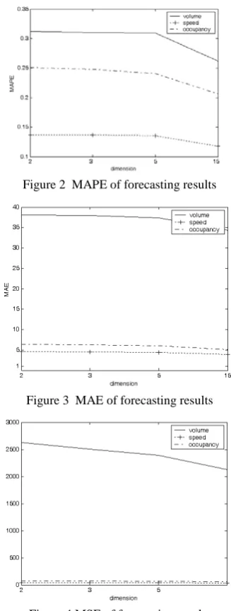
number MAPE MAE MSE 2 0.3123 38.09 2629.40 3 0.3099 37.90 2507.73 5 0.3092 37.32 2394.04 15 0.2617 34.34 2128.12
Table 5 forecasting result of speed with SVM Dimension
number MAPE MAE MSE 2 0.1371 4.60 37.40 3 0.1366 4.51 36.78 5 0.1352 4.44 35.37 15 0.1181 3.97 29.93 Table 6 forecasting result of occupancy with SVM Dimension
number MAPE MAE MSE 2 0.2512 6.40 76.74 3 0.2479 6.26 72.89 5 0.2405 5.98 66.54 15 0.2063 5.14 54.10
5.5 Forecasting with common used method
For comparison, the samples are analyzed with average value and multiple linear regression methods. 5.5.1 Average value method
We take used of previous 15 time point’s traffic flow parameters X1,X2,,X15 to forecast the current time
point’s traffic flow parameter Y . The forecasting equation is
Y=(X1+X2++X15)/15
It doesn’t need history data to determine the calculation model. The forecasting errors are shown as in table 7.
Table 7 forecasting result of Volume based on average method Parameter MAPE MAE MSE
volume 0.2899 37.53 2477 speed 0.1423 4.94 40.48 occupancy 0.3440 7.85 124.89
5.5.2 Forecasting with multiple linear regression
Let variable Y be dependent variable and , be independent variables. The regression equation is
31048 samples are used as training samples to determine the regression parameters with minimum least square methods. The left 20699 samples are used to test. The forecasting errors are shown as in table 8.
Table 8 forecasting result of occupancy with SVM with multiple regression method
parameter MAPE MAE MSE Volume 0.2841 37.10 2366.3
Speed 0.1346 4.64 35.99 occupancy 0.2464 6.09 68.16
5.6 Results analysis
The computation cost of training time and MDS processing time are shown as in figure 1. From the analysis results we can find the computation cost can be decreased markedly with the decrease of dimension number. It illustrates that feature extraction is efficient in traffic flow forecasting.
Figure 1 computation time based on different dimension number
The test results of different traffic parameters are shown as in figure 2, 3 and 4. From the results we can found that forecasting precision based on SVM is higher than that of classical forecasting methods. Although the
2 3 5 15 0
50 100 150 200 250 300
dimension
c
om
put
at
ion t
im
e
forecasting precision based on dimension reduction is decreased, it is still higher or similar to that of classical method. The affection of the reduction method is not marked in the sample is because that the dimension of input is not very higher.
Figure 2 MAPE of forecasting results
Figure 3 MAE of forecasting results
Figure 4 MSE of forecasting results
6 Conclusions
How to improve the forecasting precision of traffic flow is still an important topic in intelligent transportation systems because of the complexity and nonlinear character. In this paper, a novel forecasting method combining MDS with nonlinear SVM to forecast traffic flow data is proposed. The MDS is used to decrease the input feature vector dimension. Interpolation MDS is used to improve the dimension reduction speed. The example analysis results show that the proposed method can improve the forecasting speed. At the same time, the forecasting precision will not decrease markedly. With the development of ITS, the input dimension of traffic flow forecasting will increase
markedly and the scale of traffic flow data will become more large. The effective of the method will be more and more important to large scale traffic flow forecasting.
Acknowledgements
This work is partially supported by national youth science foundation (No. 61004115), national science foundation (No. 61272433), and Provincial Fund for Nature project (No. ZR2010FQ018).
References
1 Yang Z S. Basis traffic information fusion technology and its application. Beijing, China Railway Publish House, 2005.
2 Wang, F, Tan G Z, Deng C. Parallel SMO for Traffic Flow Forecasting. Applied Mechanics and Materials, 2010, 20(1): 843-848
3 Stephen C. Traffic Prediction Using Multivariate Nonparametric Regression. Journal of Transportation Engineering, 2003, 129(2): 161-168.
4 Cortes C, Vapnik V. Support Vector Networks[J]. Machine Learning, 1995, 20: 273–297.
5 Chang C C, Lin C J. LibSVM: a library for support vector machines. ACM Transactions on Intelligent Systems and Technology, 2001, 2(3): 1--27.
6 Hong, W C. Application of seasonal SVR with chaotic immune algorithm in traffic flow forecasting. Neural Computing & Applications; 2012, 21(3): 583-593
7 Jolliffe, I. T. Principal component analysis. New York: Springer, 2002.
8 George K M. Self-Organizing Maps. INTECH, 2010 9 Borg I, Patrick J F. Modern Multidimensional Scaling:
Theory and Applications. New York : Springer, 2005: 207– 212
10 Seung-H B, Judy Q, Geoffrey F. Adaptive Interpolation of Multidimensional Scaling. International Conference on Computational Science, 2012: 393-402
Zhanquan Sun,Ph.D, associated professor of Shandong Computer Science Center. Major on intelligent transportation systems, data mining and cloud computing. Has presided and attended 10 research projects and published about 40 academic papers.