University of Southern Queensland
Faculty of Engineering and Surveying
The Finite Difference Time Domain Method for
Computational Electromagnetics
A dissertation submitted by
CHAN, Auc Fai
in fulfillment of the requirements of
Courses ENG4111 and 4112 Research Project
towards the degree of
Bachelor of Engineering (Electrical and Electronic)
i
Abstract
Three computer programs are presented in this dissertation. The first one is a one-
dimensional (1D) program, simulating a sinusoidal signal propagating along the
x-axis. The second one is a two-dimensional (2D) program, simulating radiation from a
narrow slit. The third one is also a 2D program, which is a simulation of a Time
Domain Reflectometer (TDR) probe.
A graphical user interface (GUI) is included in the 1D program, which makes the
computer program user-friendly. A flowchart with details is included in the
appendices.
When applying FDTD to problems where solution regions are unbounded, difficulty
arises. Since no computers can store unlimited amount of data, it is necessary to
somehow, limit the solution regions. Mur’s first-order absorbing boundary condition
(ABC) is a method to achieve this. The derivation of Mur’s ABC is given in details in
Chapter Four, and implemented in the 1D program. This program serves as an
introduction to FDTD.
The 2D program simulating radiation from a narrow slit has two interesting aspects.
The perfectly matched layer (PML) is expected to absorb all electromagnetic (EM)
waves. No EM waves are supposed to pass through a perfect electric conductor
(PEC). Surprisingly, EM waves do penerate through the connecting points between
PEC and PML. The reason and solution for this ‘leakage’ are given in this
dissertation. Also one might find it a bit confusing to observe that in this program, the
x-component of electric field seems to be propagating along the y-direction. The
clarification is given in this dissertation.
University of Southern Queensland
Faculty of Engineering and Surveying
---ENG4111 & ENG4112
Research Project
---Limitations of Use
The Council of the University of Southern Queensland, its Faculty of Engineering
and Surveying, and the staff of the University of Southern Queensland, do not accept
any responsibility for the truth, accuracy or completeness of material contained
within or associated with this dissertation.
Persons using all or any part of this material do so at their own risk, and not at the
risk of the Council of the University of Southern Queensland, its Faculty of
Engineering and Surveying or the staff of the University of Southern Queensland.
This dissertation reports an educational exercise and has no purpose or validity
beyond this exercise. The sole purpose of the course pair entitled “Research Project”
is to contribute to the overall education within the student’s chosen degree program.
This document, the associated hardware, software, drawings, and other material set
out in the associated appendices should not be used for any other purpose: if they are
so used, it is entirely at the risk of the user.
Professor R Smith
Dean
iii
Certification
I certify that the ideas, designs and experimental work, results, analyses and
conclusions set out in this dissertation are entirely my own effort, except where
otherwise indicated and acknowledged.
I further certify that the work is original and has not been previously submitted
for assessment in any other course or institution, except where specifically stated
.
CHAN, Auc Fai
Student Number: 0031138976
__________________________________
Signature
Acknowledgements
The computer programs in this dissertation are modifications of programs written by
Dr. Susan C. Hagness supplied with the book Computational Electrodynamics. The
authors of the book are Dr. Allen Taflove and Dr. Susan C. Hagness.
v
Table of Contents
Page
Abstract
i
Disclaimer
ii
Certification
iii
Acknowledgments
iv
List of Figures
viii
List of Appendices
x
Abbreviations
xi
Chapter 1: Introduction
1.1
Background Information
1
1.2
Finite Element Method (FEM)
3
1.3
Method of Moments (MOM)
4
1.4
Finite Difference Time Domain (FDTD) method
5
1.5
Broad Aims and Specific Objectives
8
1.6
Dissertation Overview
8
Chapter 2: Literature Review of FDTD
2.1
Introduction
10
2.2
Conformal Transformations
11
2.3
Separation of Variables
14
2.4
Numerical Dispersion and Stability
15
2.5
Incident Wave Source Conditions
17
2.6
Soil Water Content Using TDR
20
2.7
Recent Development of FDTD
21
2.8
Recent Trends on the Development of FDTD 23
Chapter 3: Review of Available FDTD Software Packages
3.1
Software Development in FDTD
24
3.2
Review on FDTD software packages
25
Chapter 4: Theory of FDTD
4.1
Yee’s Algorithm
28
4.2
Stability Condition
31
4.3
Absorbing Boundary Conditions (ABCs)
33
4.4
Determination of Sampling Rate
38
Chapter 5: Application of FDTD to One-Dimensional ABC
5.1
Introduction
39
5.2
Modifications
39
5.3
User Guide
40
5.4
The Graphical User Interface (GUI)
51
Chapter 6: Application of FDTD to Radiation from a Narrow Slit
6.1
Introduction
53
6.2
General Features of the Seven Programs
53
6.3
Explanation of Slit Width and Huygen’s Principle
63
6.4
Further improvement in programs
68
6.5
The Program fdtd2d_gaussian_planewave
74
6.6
Directions of Propagation
75
Chapter 7: Application of FDTD to Time Domain Reflectometer
(TDR)
7.1
Introduction
80
7.2
The TDR Probe Structure
81
7.3
Calculation of the Time-Constant, T
81
7.4
Program Result
83
7.5
Removal of Leakage in TDR probe
85
7.6
Generation of a Plane Wave using Point Source
86
Chapter 8: Suggestions for Further Work and Conclusions
8.1
Suggestions for Further Work
88
vii
List of References
92
Appendices
97
Appendix A
98
Appendix B
100
Appendix C
137
Appendix D
240
List of Figures
Title
Page
Figure 2.1
Conformal Transformation
12
Figure 2.2
Conformal Transformation from a uniform field to fringing of
capacitor
14
Figure 4.1
Positions of the field components in a unit cell of the Yee’s
lattice
29
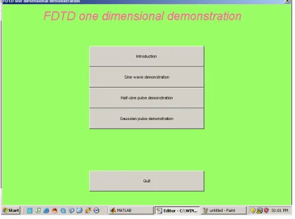
Figure 5.1
Main screen
41
Figure 5.2
Flow chart of main menu
42
Figure 5.3
Sine wave menu
43
Figure 5.4
Sample waveforms
44
Figure 5.5
Illegal inputs
45
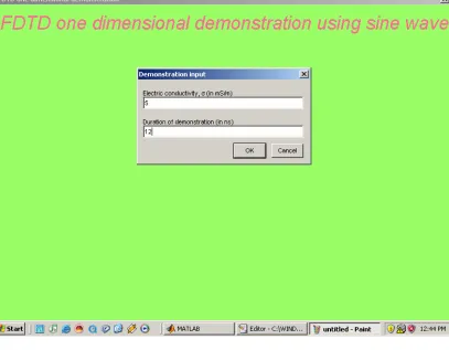
Figure 5.6
Request dialog
45
Figure 5.7
Replay dialog
46
Figure 5.8
Prompt for saving demonstration
47
Figure 5.9
Dialog for entering file name
48
Figure 5.10
Request for overwriting existing file
49
Figure 5.11
Half-sine pulse menu
50
Figure 5.12
Gaussian pulse menu
51
Figure 5.13
Flowchart of main menu
52
Figure 6.1
Snapshots of movie from onewl1.m
55
Figure 6.2
Snapshots of movie from onewl2.m
56
Figure 6.3
Snapshots of movie from onewl3.m
57
Figure 6.4
Snapshots of movie from onewl4.m
58
Figure 6.5
Snapshots of movie from twowl2.m
59
Figure 6.6
Snapshots of movie from threewl3.m
60
Figure 6.7
Snapshots of movie from PEC2.m
61
Figure 6.8
Leakage from PEC
62
Figure 6.9
Structure with a slit
64
Figure 6.10
Position of PML origin and propagation of E
x69
ix
Figure 6.13
Snapshots of movie from onewl2_new.m
72
Figure 6.14
Snapshots of movie from onewl1_wall.m
72
Figure 6.15
Snapshots of movie from onewl2_wall.m
73
Figure 6.16
Plane wave using bandpass Gaussian pulse
74
Figure 6.17
E
xin free space
78
Figure 6.18
E
yin free space
78
Figure 6.19
H
zin free space
79
Figure 7.1
A TDR System
80
Figure 7.2
The TDR Probe Structure
81
Figure 7.3
Raised-cosine step function
82
Figure 7.4
Snapshots of movie from fdtd2d_tdr_ver1.m
83
Figure 7.5
Leakage from TDR probe
84
Figure 7.6
Snapshots of movie from fdtd2d_tdr_ver2.m
85
Figure 7.7
The Modified TDR Probe Structure
86
Figure 7.8
Snapshots of movie from fdtd2d_tdr_ver3.m
87
Figure 8.1
Simulation of a sinusoidal wave hitting a dielectric medium
88
Figure 8.2
Simulation of a sinusoidal wave hitting lossy dielectric
List of Appendices
Number Title
Page
A
Project Specification
98
B
One-dimensional FDTD simulation of ABC source code
100
C
Two-dimensional FDTD simulation of radiation from a narrow
slit excited by a bandpass pulse source code
137
D
Two-dimensional FDTD simulation of TDR excited by a raised
cosine time waveform source code
240
xi
Abbreviations
1D :
One-Dimensional
2D :
Two-Dimensional
3D :
Three-Dimensional
ABC :
Absorbing Boundary Condition
EM:
Electromagnetic
FDTD :
Finite-Difference Time-Domain
FEM:
Finite Element Method
GUI :
Graphical User Interface
MOM :
Method of Moments
PEC :
Perfect Electric Conductor
PML :
Perfectly Matched Layer
RF:
Radio Frequency
Chapter 1: Introduction
1.1
Background Information
James Clerk Maxwell formulated Maxwell’s equations in 1873 (Umashankar &
Taflove, 1995). Exact analytical solutions of Maxwell’s equations were limited to
simple and symmetrical structures. Some classical methods of obtaining analytical
solutions included separations of variables and conformal transformations.
Separation of variables is applied only to electrically small shapes that can be fitted
into ortho-normal coordinate systems. For this reason, separation of variables has
limited usage on solving electromagnetic problems.
Conformal transformation is useful for analytical solution of Laplacian fields with
complicated shape. The chief limitation in this method is that equipotential boundaries
coincident with flux line are assumed. The other major disadvantage of this method is
to find a suitable transformation equation that converts a simple boundary into the
complicated boundary containing the required field to be solved.
In 1881, Rayleigh succeeded in solving exactly, the scattering of an electromagnetic
wave by a perfect conducting cylinder. In 1891, an approximate method was devised
by Kirchoff for the diffraction through a hole in a thin screen.
FDTD Method for Computational Electromagnetics
Chapter 1: Introduction
2
In 1960s, the advancement of computer technology and the increase of military
defense and industrial needs prompted the researchers to investigate the use of
numerical methods on solving electromagnetic problems (Umashankar & Taflove,
1995). Some of the popular numerical methods are methods of moments (MOM),
finite element methods (FEM) and finite difference time domain method (FDTD).
1.1.1
Classical methods to solve Maxwell’s equations
The classical methods to solve Maxwell’s equations are conformal transformations
and separation of variables.
a)
Conformal Transformations
The analytic function,
)
v
,
u
(
jy
)
v
,
u
(
x
)
t
(
f
z
=
=
+
defines a complex variable z = x+jy as a function of another complex variable
t = u+jv.
Transformations described by the above general equation are called conformal
transformations.
A detailed description of conformal transformations is given in Chapter 2: Literature
Review.
Here in this section, only the limitations and difficulty of conformal transformations
are emphasized.
The limitation of conformal transformations is that, boundaries have to coincide with
equipotential lines or flux lines inclusively; i.e. boundaries have to either coincide
with equipotential lines, or coincide with flux lines, or coincide with both
equipotential and flux lines (Binns, Lawrenson & Trowbridge 1994, pp. 121-122).
It is also rather difficult to find the transformation equation that converts a simple
boundary into more complicated boundary containing the field which is required to
solve (Binns, Lawrenson & Trowbridge 1994, p.125).
b)
Separation of variables
To obtain the analytical solution of Laplace’s equation
,
1
y
u
x
u
2 22 2
=
∂
∂
+
∂
∂
let u to be the product of two functions,
u(x,y) = X(x) Y(y)
Separation of variables means assuming that, the solution for u is the product of two
functions, one of which is a function of x only, and the other is a function of y only.
Again, detailed description of separation of variables is given in Chapter 2: Literature
Review, and only the limitation is emphasized here.
The separation of variables can only be applied to problems that fit into orthonormal
coordinate systems. This type of problems are limited in number (Umashankar &
Taflove 1993, p.2).
1.1.2
Numerical Methods to solve Maxwell’s equations
In order to overcome the limitations of classical methods, numerical methods were
developed. The commonly used methods are finite element methods (FEM), methods
of moments (MOM) and finite difference time domain (FDTD) methods.
1.2
Finite Element Method (FEM)
The origin of FEM traced back to Courant in 1943, who used triangular elements and
the principle of minimum potential energy, in the appendix of his paper (Huebner,
Thornton & Byron 1995, p.9) also (Volakis, Chatterjee & Kempel 1998, p.65).
FDTD Method for Computational Electromagnetics
Chapter 1: Introduction
4
The advantage of FEM is its capability to handle problems of complex geometries and
inhomogeneous materials (Sadiku 2003, p.377).
FEM analysis of problems involves the following steps:
•
defining the problem’s computational domain;
•
choosing the shape of discrete elements;
•
generation of mesh (preprocessing);
•
applying wave equation on each element;
•
for statics, applying Laplace’s/Poisson’s equations on each element;
•
applying boundary conditions;
•
assembling element matrices to form overall sparse matrix;
•
solving matrix system;
•
postprocessing field data to extract parameters, such as capacitance, impedance,
radar cross section and so on (Volakis, Chatterjee & Kempel 1998, p.68).
1.3
Method of Moments (MOM)
Consider the following inhomogeneous equation
g
L
ϕ
=
where L is an operator which can be differential or integral; g is the known excitation
or source function; and
ϕ
is the response or unknown function to be found. It is
assumed that L and g are given and the task is to determine
ϕ
(Harrington 1993, pp.
1-2).
The procedure of solving the above equation as presented by Roger F. Harrington is
called method of moments. The procedure expands
ϕ
as a series of functions
∑
ϕ
=
ϕ
and multiples
ϕ
by a set of weighting functions w
nand finally solves for a
n(Harrington 1993, pp. 5-6).
In other words, MOM reduces
L
ϕ
=
g
into matrix equations by using a method
known as the method of weighted residuals.
MOM has been successfully used to model:
•
scattering by wires and rods;
•
scattering by two-dimensional (2D) metallic and dielectric cylinders;
•
scattering by three-dimensional (3D) metallic and electric objects of arbitrary
shapes; and
•
many other scattering problems.
MOM requires significant computer memories (Umashankar & Taflove 1993, p.4)
also (Sadiku 2003, p.285).
MOM is not suitable for analyzing the interior of conductive enclosures (Todd 1991,
p.7).
1.4
Finite Difference Time Domain (FDTD) method
FDTD Method for Computational Electromagnetics
Chapter 1: Introduction
6
The basic algorithm of FDTD was first proposed by K.S. Yee in 1966. In 1975, Allen
Taflove and M.E. Brodwin obtained the correct criterion for numerical stability for
Yee’s algorithm and, firstly solved the sinusoidal steady-state electromagnetic
scattering problems, in two- and three-dimensions. This solution becomes a classical
computer program example in many FDTD textbooks. Many researchers follow; and
among them are G. Mur and J.P. Berenger. Mur published the first numerically stable
absorbing boundary condition (ABC) in 1981. Berenger introduced, the best ABC for
the time being, the perfectly matched layer (PML) in 1994.
1.4.1
Comparison between FDTD and FEM
FDTD is good for Radio Frequency (RF) and microwave applications. It is not too
difficult to write computer programs to implement FDTD and there is no need to
solve matrix equations. The final results of FDTD computer programs are displayed
in movies and therefore easy to understand, and good for physical insight. As a result,
FDTD is suitable for teaching purposes.
FEM is more suitable for low frequency of 50 Hz. It uses fewer elements than FDTD.
FEM needs more preprocessing and postprocessing, as mentioned in section 1.2.
1.4.2
Comparison between FDTD and MOM
FDTD permits the modeling of electromagnetic wave interactions with a level of
detail as high as that of MOM. For FDTD, the overall computer storage and running
time requirements are linearly proportional to N, the number of field unknowns, but
MOM requires more storage and running time. MOM leads to systems of linear
equations having dense, full coefficient matrices, which require computer storage
proportional to N
2, N being the number of field unknowns. The computer execution
time to invert the MOM system matrix has N
2to N
3dependence (Umashankar &
Taflove 1993, pp. 4-5).
1.4.3
Comparison between FDTD and Frequency-Domain
Techniques
After 1960, the advent of digital computers enabled the frequency-domain techniques
to become quite sophisticated. In this period, the main computational approaches for
Maxwell’s equations were high-frequency asymptotic methods and integral equations,
both being frequency-domain techniques.
However, these frequency-domain techniques have many shortcomings.
Asymptotic method is suitable for modeling the scattering properties of electrically
large complex shapes. However, if has difficulty in treating nonmetallic material
composition, and volumetric complexity of a structure.
Integral equations can handle material and structural complexity. However, they lead
to systems of linear equations, which limits the electrical size of possible models.
Although progress has been made in solving huge systems of equations generated by
frequency-domain integral equations, the capabilities of even the latest technologies
to solve them, are exhausted by many structures of engineering interest (Taflove &
Hagness 2000, pp. 3-4).
1.4.4
Justification for the Use of FDTD
In 1970s and 1980s, researchers realized the limitations of frequency-domain
techniques. This led to an alternative approach: the FDTD.
The advantages of FDTD are as follows:
•
Frequency-domain integral-equation and finite-element methods can model
10
6electromagnetic field unknowns. FDTD can model 10
9unknowns.
•
In FDTD, specifying a new structure is only a problem of mesh generation,
which is much easier than the complex reformulation of an integral equation.
FDTD Method for Computational Electromagnetics
Chapter 1: Introduction
8
1.5
Broad Aims and Specific Objectives
The aims of this project are to search in the Internet for available software for solving
electromagnetic problems, and to write computer programs to display the phenomena
of electromagnetic wave propagations in the form of movies for the purpose of
teaching.
The specific objectives are:
(a)
to write a one-dimensional Finite Difference Time Domain (FDTD)
simulation of Absorbing Boundary Condition;
(b)
to write a two-dimensional FDTD simulation modeling the radiation from a
narrow slit excited by a plane wave which is a bandpass pulse;
(c)
to write a two-dimensional FDTD simulation of a Time Domain Reflectometer
probe (TDR) excited by a DC pulsed plane wave having a raised cosine time
waveform.
1.6
Dissertation Overview
The first chapter is to provide the background information about the historical
development of solutions for Maxwell’s equations. The project aims and objectives
are also specified.
Chapter 2: Literature Review is to acquire enough knowledge about FDTD to support
the computer programming in FDTD.
Chapter 4: Theory of FDTD is a brief description of all the theories required before
the programs are designed and constructed.
Chapter 5: Application of FDTD to one-dimensional ABC is about 1D-computer
programs. It is a good introduction to FDTD, and is useful as a training exercise.
Chapter 6: Application of FDTD to Radiation from a Narrow Slit is to write a
program to show a 2D model of radiation from a narrow slit excited by a plane wave,
which is a bandpass pulse.
Chapter 7: Application of FDTD to Time Domain Reflectometer (TDR) is to simulate
a 2D model of a TDR probe of given geometry.
FDTD Method for Computational Electromagnetics
Chapter 2: Literature Review
10
Chapter 2: Literature Review of FDTD
2.1
Introduction
The objectives of this literature review are to acquire enough knowledge about FDTD
to support the computer programming in FDTD, and to acquire knowledge relevant to
this project.
The central part of this literature review, the theory of FDTD, because of its
importance, deserves a single chapter. It is described in Chapter 4.
A summary of sections in this review are given below :
Section 2.2 Conformal Transformations, and section 2.3 Separation of Variables, are
analytical methods for solving Maxwell’s equations. These two sections present
introductions to these two methods.
Section 2.4 Numerical Dispersion and Stability, and section 2.5 Incident Wave Source
Conditions, are book reviews on Computational Electrodynamics, by A. Taflove and
S.C. Hagness.
Allen Taflove has pioneered the FDTD method since 1975 (the year in that he
published his PhD dissertation), and is a leading authority in FDTD. He is one of the
most-cited researchers in FDTD (Taflove & Hagness, 2000).
Therefore reading of Taflove’s book is essential. Two of the chapters from the book
are presented in literature review.
Section 2.6 Soil Water Content Using TDR, is a review on a research paper. The
paper “Electromagnetic Determination of Soil Water Content Using TDR,” by Topp
et al., 1982, inspired the part on TDR, of this project.
2.2
Conformal Transformations
When there are no charges in space, the differential form of Gauss’ law is,
Div E = 0
Furthermore, in a purely electrostatic field, E may be expressed as minus the gradient
of the potential U:
E = -grad U
Therefore
div grad U = 0
It is convenient to think of div grad as a single differential operator, which is called
the Laplacian.
Laplacian U = 0,
which is Laplace’s equation.
Laplace’s equation can be solved analytically by conformal transformations.
The analytic function,
)
v
,
u
(
jy
)
v
,
u
(
x
)
t
(
f
z
=
=
+
defines a complex variable z = x+jy as a function of another complex variable
t = u+jv.
Transformations described by the above general equation, are called conformal
transformations.
Let us consider an example of conformal transformation.
Suppose
z = sin t
It has already been defined that z = x+jy and t = u+jv
Therefore
x+jy = sin t
= sin(u+jv)
= sin u cos jv + cos u sin jv
= sin u cosh v + jcos u sinh v
Equating the real and imaginary parts,
FDTD Method for Computational Electromagnetics
Chapter 2: Literature Review
12
Squaring and adding these equations eliminates u, giving
,
1
v
sinh
y
v
cosh
x
2 2
2 2
=
+
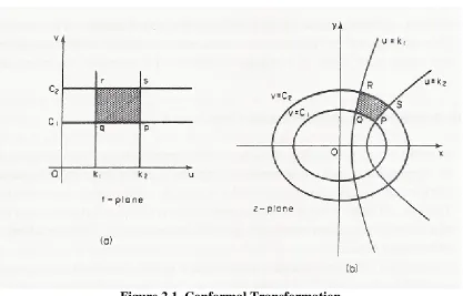
which is the equation of an ellipse.
Squaring and subtracting them eliminates v, so that
,
1
u
cos
y
u
sin
x
2 2
2 2
=
−
which is the equation of a hyperbola.
[image:24.595.90.507.311.578.2]Therefore a straight line described by v = constant is transformed into an ellipse;
while a straight line described by u = constant is transformed into a hyperbola.
Figure 2.1 Conformal Transformation
Properties of conformal transformations are summarized below:
•
For any two intersecting curves, the angle of intersection is unaltered by the
conformal transformation.
•
To pass from one arm of the angle to the other arm, one must travel around the
point of intersection in the same sense.
•
If an analytic function satisfies Laplace’s equation in some region R’ of the
t-plane, the transformation of that analytic function still satisfies Laplace’s equation
in the appropriate region R of the z-plane.
•
Expressing in another way, if possible to find a solution of Laplace’s equation in a
region of the t-plane, then the same function expressed in terms of x, y in the
plane will be a solution of Laplace’s equation in the transformed region in the
z-plane.
(Binns, Lawrenson & Trowbridge 1995, pp.117-122)
(Sokolnikoff & Redheffer 1958, pp.576-586)
(Jeffreys & Swirles 1966, pp.409-411)
2.2.1
Example of Conformal Transformation
Let us have an example to illustrate how conformal transformation can be applied to
solve the flux fringing at the end of a parallel plate capacitor.
Consider first the complex plane t where there is a uniform electric field. The lines u
= constant are flux lines, while the lines v = constant are equipotential lines. This
uniform field is the simplest Laplacian field to which all other solutions are related.
The following conformal transformation will transform the uniform field to flux
fringing at the end of the capacitor.
z = t + e
t(This transformation is stated without proof here. Proof is given in
The
Analytical and Numerical Solution of Electric and Magnetic Fields
, but it is beyond
the scope of this dissertation. The proof presented in the Book, and also the equation
log z = log t + t log e = log t + t useful.)
Therefore x + jy = (u + jv) + e
u+jv= (u + jv) + (e
u) (e
jv)
FDTD Method for Computational Electromagnetics
Chapter 2: Literature Review
14
Equating the real and imaginary parts,
x = u + e
ucos v
y = v + e
usin v
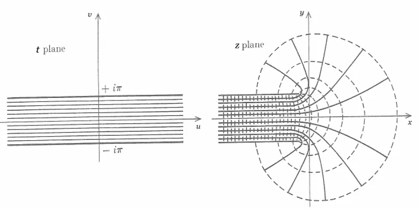
[image:26.595.92.503.178.383.2]A plot of x, y gives the fringings.
Figure 2.2 Conformal Transformation from a uniform field to fringing of
capacitor
(Sokolnikoff & Redheffer 1958, p.586; Binns, Lawrenson & Trowbridge 1995,
pp.155-157)
2.3
Separation of Variables
Unlike conformal transformation, which can only be found in textbooks of advanced
level, separation of variables can be found in almost any textbooks on
electromagnetics.
To obtain the analytical solution of Laplace’s equation
,
1
y
u
x
u
2 22 2
=
∂
∂
+
∂
∂
Hence
0
dy
Y
d
Y
1
dx
X
d
X
1
2 2 2 2=
+
Putting
2 2 2dx
X
d
X
1
ϖ
−
=
and
2 2 2dy
Y
d
Y
1
ϖ
=
where
ϖ
is any real number,
,
y
sinh
D
y
cosh
C
Y
,
x
sin
B
x
cos
A
X
ϖ
+
ϖ
=
ϖ
+
ϖ
=
A, B, C and D being arbitrary constants.
The solution is
u(x,y) = XY
)
y
sinh
D
y
cosh
C
)(
x
sin
B
x
cos
A
(
ϖ
+
ϖ
ϖ
+
ϖ
=
(Rao 2004, pp.726-728; Binns, Lawrenson & Trowbridge 1995, pp.57-58)
2.4
Numerical Dispersion and Stability
This is a summary of Chapter 4, of
Computational Electrodynamics
by A. Taflove
and S.C. Hagness.
In the FDTD algorithm, numerical dispersion and stability are the two main factors
that affect the choice of time step,
Δ
t and lattice space increments,
Δ
x ,
Δ
y and
Δ
z .
In a uniform one-dimensional grid, numerical dispersion is reduced to ideal
dispersion, when the magic time-step is used. That is, the Courant factor S, is 1.
Under this condition, the solution of a continuous one-dimensional wave equation,
given by the Yee algorithm, is exact.
FDTD Method for Computational Electromagnetics
Chapter 2: Literature Review
16
Along the diagonal of a two-dimensional square grid, if S is
1
2
, numerical
dispersion reduces to ideal dispersion.
Similarly, along the diagonal of a three-dimensional cube grid, if S is
1
3
,
numerical dispersion reduces to ideal dispersion.
The numerical dispersion error can be quantified by the physical phase-velocity error
and the velocity-anisotropy error.
Physical phase-velocity error measures the amount of phase lead or lag.
Velocity-anisotropy error measures the wavefront distortion due to the Velocity-anisotropy of the space
lattice. Physical phase-velocity error can be reduced by proper choice of grid
discretization.
Stability problem becomes complex when the Yee algorithm is used with :
1.
boundary conditions;
2.
variable and unstructured meshing; and
3.
lossy, dispersive, nonlinear, and gain materials.
In this book, four strategies are suggested to reduce the effect of numerical dispersion
in the Yee algorithm.
These strategies are:
1.
to create a specific numerical phase-velocity curve about c;
2.
to use fourth-order-accurate spatial differences;
3.
to use hexagonal grids; and
Short descriptions on these four strategies are given below.
§
Centre a specific numerical phase-velocity curve about c
The physical phase-velocity can be reduced by shifting the phase-velocity curve
so that it is centred about c, the speed of light in free-space. However, the
velocity-anisotropy remains unchanged.
§
Fourth-order accurate spatial differences
The phase-velocity anisotropy error can be reduced by using
fourth-order-accurate finite difference scheme in the Yee algorithm. Also, under this situation,
the computer storage is greatly reduced. The only drawback is large stencil
needed to calculate fourth-order spatial differences when dealing with material
interfaces.
§
Use Hexagonal grids
Hexagonal grids exhibit a fourth-order dependence, in spite of the second-order
accuracy of spatial difference being used.
Difficulties arise when hexagonal grids are used in three dimensions. An
automated computer-based mesh generation is needed.
Hexagonal grid, in comparison with fourth-order-accurate spatial differences, has
lower numerical dispersion. Hence, less computer storage is required.
§
Use Discrete Fourier Transform to calculate the spatial derivatives
Pseudo-spectral time-domain (PSTD) method is used on unstaggered, collocated
Cartesian space lattices. The velocity-anisotropy error is reduced to zero.
However, PSTD can only be used in structures comprised entirely of dielectrics.
2.5
Incident Wave Source Conditions
This is a summary of Chapter 5, of
Computational Electrodynamics
, by A. Taflove
and S.C. Hagness.
FDTD Method for Computational Electromagnetics
Chapter 2: Literature Review
18
Four kinds of electromagnetic wave sources are discussed. They are:
•
hard-sourced E and H fields in one-and two-dimensional grids;
•
J and M sources in three-dimensional lattices;
•
total-field/scattered-field formulation for plane-wave excitation in one, two, and
three dimensions; and
•
waveguide sources.
2.5.1
Hard sources in one dimension
A hard source can be set up by using an analytical time-domain function at specific
components of E and H in the FDTD space lattice.
For a pulsed hard source or continuous sinusoidal wave, established at grid-point
i
s,
the reflected wave from a material structure will eventually return to i
s.
At i
sthe total tangential E-field is specified without considering any possible reflected
waves in the grid. The hard source generates purious, nonphysical/retroreflection
waves at i
s, back to the material structure.
This problem can be solved by turning off the hard source before any reflected waves
reach the hard source. However, this will limit the maximum number of time steps in
FDTD simulation.
2.5.2
Hard sources in two dimensions
After careful analysis, it is found that a “pointwise” hard source in two dimensions is
not a point. The hard source has a finite effective radius of approximately 0.2 grid cell
in two-dimensional FDTD models, when the grid cell size,
Δ
is much less than
10
0
2.5.3
J
and
M
current sources in three dimensions
Yee space lattice is divergence-free in free-space regions when there is no
J and M
sources. However, current sources having specific geometry and temporal property
can deposit charges in the Yee lattice.
Since Yee lattice can deposit electric and magnetic charges, it is possible to calculate
the capacitance and inductance between cells of the space lattice.
After some calculation, the intrinsic lattice capacitance and inductance between
adjacent FDTD space lattice in free space are found to be
3
ε
0Δ
and
4
Δ
0
µ
respectively, where
Δ
is the length of a cubic-cell.
When a lumped-element capacitor or a lumped-element inductor is added at a specific
point within the FDTD space lattice, the total capacitance or inductance at that point
is the sum of the intrinsic lattice capacitance or inductance plus the lumped-element
capacitance or inductance.
2.5.4
The total-field/scattered-field technique
The total-field/scattered-field (TF/SF) attempt to model a plane-wave source by using
the linearity of Maxwell’s equations.
The total electric and magnetic fields E
totaland H
totalare assumed to be decomposed in
the following manner:
E
total= E
inc+ E
scatH
total= H
inc+ H
scatE
incand
H
incare the known incident-wave fields that exist in vacuum without any
materials in the space lattice.
FDTD Method for Computational Electromagnetics
Chapter 2: Literature Review
20
When the Yee algorithm is applied across the interface, inconsistency arises because
of the arithmetic difference between scattered- and total-field values. Correction can
be made by using the fact that the total-field value is the sum of the incident-field and
scattered-field values.
For two-dimensional and three-dimensional problems, the calculation of the incident
field is simplified by a table look-up procedure.
2.5.5
Total-field/reflected-field model formulation for waveguide system
The method used in waveguide system is similar to that used in the TF/SF technique.
Region 1 is the total-field region and it contains the interacting structures of interest.
Region 2 contains only the reflected-field and the absorbing boundary condition. The
consistency condition at the interface between Region 1 and Region 2 is corrected by
using the similar procedures in TF/SF technique.
The total-field/reflected-field programming for a waveguide can be adapted from the
TF/SF technique.
2.6
Soil Water Content Using TDR
The technology of Time-Domain Reflectometry (TDR) was applied in vertical
transmission lines constructed by using parallel wires. The transmission lines were
inserted vertically into soil. It was found that this method gave a good measure of the
soil water content (Topp et al. 1982, p.678).
This paper inspired the third computer programming on TDR in this project
2.7
Recent Developments of FDTD
Descriptions of seven journal papers were given below.
i)
The first paper, A New FDTD Algorithm Based on Alternating-Direction
Implicit (ADI) Method, by Takefumi Namiki, was published in 1999. The
ADI method removes the Courant-Friedrich-Levy (CFL) condition. Two
simulation examples are given.
The first example is a 2D free-space simulation, with Mur’s first-order ABC and a
sine-wave (squared and then added to the source position, i.e. soft source). The results
are given below.
For conventional FDTD:
delta t = 9.4 ps
number of time-steps = 5000
CPU time = 215.5s
computer memory = 429.8 Kb
For ADI:
delta t = 235.0 ps
number of time-steps = 200
CPU time = 27.5s
computer memory = 566.7 Kb
The ADI, after removing Courant condition, has larger delta t, so less time-steps and
CPU time. It is faster.
FDTD Method for Computational Electromagnetics
Chapter 2: Literature Review
22
ii)
The second paper, Toward the Development of a Three-Dimensional
Unconditionally Stable Finite-Difference Time-Domain Method, by Fenghua
Zheng, Zhizhang Chen, and Jiazong Zhang, was published in 2000. This is a
modification of ADI, and an extension from 2D to 3D.
iii)
The third paper, the Concurrent Complementary Operators Method for FDTD
Mesh Truncation, by Omar M. Ramahi, was published in 1998. This paper
introduced a new absorbing boundary condition.
iv)
The fourth paper, Numerical Dispersion Analysis of the Unconditionally
Stable 3-D ADI-FDTD Method, by Fenghua Zheng and Zhizhang Chen, was
published in 2001. This is related to the second paper. It continues to discuss
the dispersion of the 3-D ADI introduced in the second paper.
v)
The fifth paper, FDTD Dispersion Revisited: Faster-Than-Light Propagation,
by John B. Schneider and Christopher L. Wagner was published in 1999. It
discusses the dispersion relation for the second-order FDTD, first derived by
Taflove.
vi)
The sixth paper, A Conformal FDTD Software Package Modeling Antennas
and Microstrip Circuit Components, was written by Wenhua Yu and Raj
Mittra.
Conventional FDTD proposed by K.S. Yee uses cubical cells in
three-dimensions and square cells in two-three-dimensions. Consequently the errors in
modeling perfect electric conductors (PECs) with curved surfaces will be
significant. Reducing the size of the cells to better fit the curve will increase
computer timing.
Wenhua and Raj Mittra proposed Conformal FDTD to handle PECs with
curved surfaces and developed a software package on Conformal FDTD
vii)
The seventh paper, An Effective PML for the Absorption of Evanescent
Waves in Waveguides, by Jean-Pierre Berenger, was published in 1998.
The abstract of this paper states that, as emphasized by several authors in
literature, the evanescent modes are not absorbed by usual PML terminating
waveguiding structures. A new version of PML, denoted as PML-D, is
presented in this paper, which substantially absorbs such waves.
2.8
Recent Trends on Development of FDTD
Based on the journal papers, the recent trends are:
•
reducing CPU time;
•
searching for new ABCs;
•
re-examining dispersion;
•
modification of conventional FDTD to handle PECs with curved surfaces;
•
development of software packages on FDTD
FDTD Method for Computational Electromagnetics
Chapter 3: Review of Available
FDTD Software Packages
24
Chapter 3: Review of Available FDTD Software
Package
3.1
Software development in FDTD
Since the introduction of FDTD approach nearly thirty years ago, FDTD had become
a popular computer technique for solving electromagnetic field problems in many
applications, ranging from the design of antennas to biophotonics.
FDTD was a relatively new method when it was compared to other computational
methods, such as finite element method or the method of moments.
FDTD commercial packages appeared later than those in FEM due to the fact that
satisfactory absorbing boundary was not available until 1994.
Many companies and educational institutes offered FDTD software packages with
free or limited usage. It was possible to convert some of the free FDTD software with
limited capability to a software with complete features after paying the license fee.
The license fee can be a yearly license or a one-time license.
Over the last decade, the development of personal computer had a great progress,
therefore the speed of computation, the accuracy of FDTD solution and the electrical
size of the electromagnetic problem increased. The speed of a personal computer
increased from 133MHz to 2.93GHz. The number of bits that a computer could
handle rose from 16 bits to 32 bits. The random access memory (RAM) increased
from 8MB to 8GB.
The increase in number of bits that a computer could handle helped to reduce the error
induced by truncation. Thus the accuracy of the FDTD simulation results had been
improved.
The electrical size of an electromagnetic problem depended on the size of RAM. With
the increase in the size of RAM, more unknown FDTD variables could be handled.
The size of a grid cell could be made smaller because of more RAM available.
Besides the new development in personal computers, dedicated hardware for FDTD
was available to improve the performance of FDTD. However, dedicated hardware
was expensive.
An alternative way to solve general-purpose FDTD problem was to use the graphic
card for FDTD computation. High performance graphic card was much cheaper than
dedicated FDTD hardware. The only problem for this approach was that pre and pro
processing were needed in transforming between FDTD data and image data.
3.2
Review on FDTD software packages
The review was given below after a survey on available FDTD software packages.
•
EZ-FDTD software package
FDTD Method for Computational Electromagnetics
Chapter 3: Review of Available
FDTD Software Packages
26
•
Fidelity- FDTD software module
Fidelity is a software module in Zealand application package. It is a software module
using FDTD to solve problems. The evaluation version of this software is
network-based software. It can only be used online. It is advisable to have internet connection
speed of more than 56Kbps if the evaluation version is used. Fidielty provides some
standard structure like waveguide, antenna, coaxial port and microstrip port. Fidielty
also provides point source and plane wave source. Fidielty can have far and short field
view. (http://www.zeland.com)
•
Empire-FDTD software package
Empire software package can be run on Windows and Linux platform. Empire
software also supports 64-bit operation. 64MB of RAM and 400MB of hard disk
space are needed for installation. For optimum operation, an Intel Pentium IV
processor with chipset, 1 GB DDR RAM at 400MHz and a graphic card with 128MB
are recommended. Near and far field plots are available. AutoCAD import and export
of design is possible. (http://www.empire.de)
•
Concerto-FDTD software module
•
XFDTD-software package
XFDTD can be run on multiple processor computers and it is able to have parallel
computation. XFDTD requires Windows 2000/XP for 32-bit operating systems. It
needs minimum 256 MB RAM. However, 512 MB (or more) RAM is recommended.
16 bit color OpenGL compliant video card (Matrox cards not supported, ATI or
NVidia cards recommended) with 1024x768 display resolution is needed. A hard disk
of 500 MB space is needed for full installation. XFDTD provides high fidelity human
meshes for biological electromagnetic simulations. The meshes can be stretched and
rotated. CAD design can be import for FDTD simulation. Utilizing the ability of the
GPU (Graphics Processing Unit) in modern computer graphics cards to stream
floating point calculations, XFDTD achieves extremely fast calculation speeds.
(http://www.remcom.com)
3.3
Conclusion
FDTD Method for Computational Electromagnetics
Chapter 4: Theory of FDTD
28
Chapter 4: Theory of FDTD
4.1
Yee’s Algorithm
In 1966, K.S. Yee published his classic research paper “Numerical solution of initial
boundary value problems involving Maxwell’s equations in isotropic media.” (Yee
1966).
Yee’s paper introduced a set of finite-difference equations for the time-dependent
Maxwell’s curl equations. Using the two Maxwell’s curl equations, Yee solved both
electric and magnetic fields in time and space, in a leapfrog manner. Yee also
introduced the Yee’s lattice, which is shown on next page Figure 4.1.
Sadiku (2003, pp. 160-163) presented the following derivation.
Maxwell’s equations in an isotropic medium are as below
A grid point in the solution region is defined as
and functions of space and time are defined as
where
δ
=
Δ
x
=
Δ
y
=
Δ
z
is the space increment; t
Δ
is the time increment;
i, j, k,
and
n
are integers. Using central finite difference approximation for space and time
derivatives, it becomes:
Yee positioned the components of E and H about a unit cell of the lattice as shown in
Figure 4.1. Every
E components is surrounded by four
H components, and every H
component is surrounded by four E components.
FDTD Method for Computational Electromagnetics
Chapter 4: Theory of FDTD
30
Equations (4.1) to (4.7) are direct reproductions from Sadiku’s book.
4.2
Stability Condition
The following is based on the book
Time-Domain Computer Analysis of Nonlinear
Hybrid Systems
by Wenquan Sui.
Sui (2001, pp.154-156) expressed that FDTD is an explicit finite-difference method.
Therefore all unknowns at present time-step are evaluated from known values at
previous time-step.
The time increment
Δ
t
in FDTD is limited by the stability requirement known as the
Courant-Friedrichs-Lewy (CFL) condition (Taflove & Hagness, 2000).
For 3D FDTD in a uniform grid, the stability requirement is:
2
2
2
Δ
z
1
Δ
y
1
Δ
x
1
v
1
t
Δ
+
+
FDTD Method for Computational Electromagnetics
Chapter 4: Theory of FDTD
32
where
v
is the propagation speed of electromagnetic wave inside the medium.
When all the cell sizes are the same,
Δ
Δ
z
Δ
y
Δ
x
=
=
=
v
Δ
577
.
0
3
v
Δ
t
Δ
≤
=
For 2D FDTD, with the same cell sizes, the stability requirement is
v
Δ
71
.
0
2
v
Δ
t
Δ
≤
=
For 1D FDTD, with the same cell sizes, the stability requirement is:
v
Δ
t
Δ
≤
A convenient time-step that satisfies the stability requirement for 1D, 2D and 3D is:
v
Δ
5
.
0
v
2
Δ
t
Δ
=
=
The equal sign “=” but not “
≤
” is used here
and 0.5 < 0.577 < 0.71 < 1
t
Δ
can be smaller, but cannot be bigger, than the stability requirement.
To obtain higher accuracy in solution, the grid size has to be smaller. Hence the
time-step will be smaller.
The spatial sampling rate is required to be between 10 samples per wavelength to 20
samples per wavelength.
For a system excited by a sinusoidal source of 3GHz, the wavelength is 0.1 meter. If
the sampling rate is 20, the cell size will be 0.1/20 = 0.5 cm.
A convenient time-step for 1D, 2D and 3D will be
12
8
/
10
3
.
8
10
3
2
20
0.1
t
Δ
=
×
−
×
×
=
second
4.3
Absorbing Boundary Conditions (ABCs)
This section consists of three sub-sections, namely the classification of ABCs, Mur’s
first-order ABC, and the perfectly matched layer (PML).
4.3.1
Classification of ABCs
Sadiku in his book,
Numerical Techniques in Electromagnetics
, page164, explains the
need to use ABCs.
Taflove in his book, Advances in Computational Electrodynamics, page 3, presents a
concise classification of ABCs.
When applying FDTD to problems where the solution regions are unbounded,
difficulty arises. Since no computers can store unlimited amount of data, it is required
to somehow, limit our solution regions. ABC is the method to limit the solution
regions and it creates the numerical illusion of an infinite space.
Most of the Absorbing Boundary Conditions (ABCs) can be grouped into two
categories. One category is ABCs derived from differential equations. The other
category is ABCs using material absorbers.
Mur’s first-order and second-order absorbing boundary conditions are examples of
ABCs derived from differential equations.
FDTD Method for Computational Electromagnetics
Chapter 4: Theory of FDTD
34
4.3.2
Mur’s first-order ABC
(a)
Mur’s first-order ABC by Common Sense Approach
Sullivan in his book, Electromagnetic Simulation Using the FDTD Method, page 4,
presents what he said ‘
a common sense approach
’.
Suppose a wave is travelling at c, the speed of light, along the negative x direction,
towards a boundary at the end of the computational domain.
If
Δ
t =
Δ
x/c, then it takes one time step for a wave front to cross
Δ
x, one cell.
Therefore, a common sense approach is:
u at next time step = u at present time step
Written in symbols, it is
(u at time step n+1, at spatial step 0) = (u at time step n, at spatial step 1)
Note that the wave is travelling from spatial step 1 to spatial step 0, along the negative
x direction.
That is u
n+1(0) = u
n(1)
It is easy to implement this ABC. Simply store the value u
n(1), and then put it at
u
n+1(0).
(b)
Mur’s first-order ABC by Derivation
The following derivation is based on the book
Computational Methods for
Electromagnetics
by A.F. Peterson, S.L. Ray and R. Mittra, page 511 to page 513.
The first order ABC developed by Mur is discussed here.
The one-dimensional wave equation is
0
t
u
c
x
u
2 2
2 2 2
1
=
−
∂
∂
∂
The wave equation can be factored by treating the differential operators algebraically.
0
t
u
c
1
x
u
t
u
c
1
x
u
=
∂
∂
+
∂
∂
∂
∂
−
∂
∂
The two brackets can be equated to zero to give the one-way wave equation
0
t
u
c
1
x
u
=
∂
∂
−
∂
∂
(4.8)
or
0
t
u
c
1
x
u
=
∂
∂
+
∂
∂
(4.9)
Solutions to Equation (4.8), u(x+ct) are –x travelling waves, while solutions to
Equation (4.9), u(x-ct) are +x travelling waves. Thus, to simulate an open-region
problem, Equations (4.8) and (4.9) are used as boundary conditions on the left and
right boundaries respectively. The above Book then jumps to the result, Equation
(4.11).
The elaborations to find the final result Equation (4.11) were given below.
Discretizing Equation (4.8), the first-order equation for negative x direction
propagating waves, is:
( )
( )
[
]
[
( )
( )
]
+
−
+
+ +0
0
2
1
1
1
2
1
x
Δ
1
u
u
u
u
n 1 n n 1 n( )
( )
[
]
[
( )
1
( )
0
]
0
2
1
0
1
2
1
x
Δ
1
c
1
u
u
u
u
n 1 n 1 n n
=
+
−
+
−
+ +(4.10)
Multiple both sides by
2
c
( )( )
Δ
t
Δ
x
( )
Δ
t
( ) ( ) ( ) ( )
1
c
Δ
t
1
c
Δ
t
( )
0
c
u
n+1+
u
n−
u
n+1( ) ( ) ( )
Δ
t
0
Δ
x
( ) ( )
1
Δ
x
( ) ( ) ( ) ( ) ( )
0
Δ
x
1
Δ
x
0
0
c
u
n−
u
n 1−
u
n 1+
u
n+
u
n=
FDTD Method for Computational Electromagnetics
Chapter 4: Theory of FDTD
36
Grouping like terms together to give
( ) ( ) ( ) ( ) ( )
Δ
t
1
Δ
x
1
c
Δ
t
( ) ( )
1
Δ
x
( ) ( ) ( ) ( ) ( )
1
Δ
x
0
c
Δ
t
0
c
u
n+
u
n+
u
n+1−
u
n+1+
u
n−
u
n( )
Δ
t
( ) ( )
0
Δ
x
( )
0
c
u
n+1+
u
n+1=
Factorizing to get
( ) ( )
0
[
c
Δ
t
Δ
x
]
u
n+1+
=
u
n( ) ( )
1
[
c
Δ
t
+
Δ
x
]
+
u
n+1( ) ( )
1
[
c
Δ
t
−
Δ
x
]
−
u
n( ) ( )
0
[
c
Δ
t
−
Δ
x
]
( ) ( )
0
[
c
Δ
t
Δ
x
]
u
n+1+
=
u
n( ) ( )
1
[
c
Δ
t
+
Δ
x
]
+
[
c
( )
Δ
t
−
Δ
x
]
[
u
n+1( )
1
−
u
n( )
0
]
( )
0
u
( )
1
[
c
( )
Δ
t
Δ
x
]
[
c
( )
Δ
t
Δ
x
]
*
[
u
( )
1
u
( )
0
]
u
n 1 n/
n 1−
n
+
−
+
=
++
(4.11)
If
c
( )
Δ
t
−
Δ
x
=
0
, the second term on the right hand side of Equation (4.11) will
vanish.
Under the condition
Δ
t
=
Δ
x
/
c
i.e. the magic step,
( )
0
u
( )
1
u
n+1=
nwhich is the same as the result obtained by common sense approach.
4.3.3
The Perfectly Matched Layer (PML)
PML is realized by surrounding the computational domain with a lossy material that
dampens the outgoing fields.
With properly designed parameters of the PML, incident waves, with any incident
angle, will penetrate into the PML without reflection, and are rapidly attenuated inside
the PML. The reflection coefficient is zero at boundaries if the parameters of the PML
have the following relation:
µ
=
ε
σ
σ
e mε
is the permittivity,
σ
mis the magnetic conductivity, and
µ
is the permeability.
The outer boundary of the PML has a perfect electric conductor (PEC) wall, which
will reflect waves back into the PML.
When the above relation is satisfied, the 2D TE mode field inside the PML is found to
be
F = F
opqr
where
F
ois the initial field
p
is exp
(
)
φ
+
φ
−
x
cos
y
sin
c
jw
jwt
q
is exp
φ
ε
−
σ
cos
c
x
xr
is exp
φ
ε
−
σ
sin
c
y
yand
ε
µ
=
2 1Ζ
The field inside the PML decreases exponentially. Since the impedance of the PML,
Ζ
, is the same as the impedance just outside the PML, incident waves, at any angle,
will transmit into the PML without reflection (Sui 2001, pp.162-163).
FDTD Method for Computational Electromagnetics
Chapter 4: Theory of FDTD
38
4.4
Determination of Sampling Rate
This section is based on the book,
Finite Difference Time Domain Method for
Electromagnetics
, by K.S. Kunz and R. J. Luebbers.
The sampling rate is usually between 10 samples per wavelength to 20 samples per
wavelength. The source, such as Gaussian pulse, may contain many wavelengths. The
wavelength in sampling rate should be the shortest wavelength in the source.
For accurate determination, such as of radar scattering cross-section, 20 samples per
wavelength are necessary. For other cases, reasonable results may be obtained by 10
samples per wavelength.
The paragraphs below present a more detailed description on sampling rate.
According to Nyquist sampling theorem, there must be at least two samples per
wavelength in order for the spatial information to be obtained.
In addition to Nyquist theorem, the grid dispersion error has to be considered. In
FDTD, waves of different frequencies propagate at slightly different speeds through
the grid. The propagation speed also depends on the direction of propagation relative
to the grid. A sampling rate of 10 to 20 samples per wavelength, will give accurate
results, under dispersion error, and satisfy Nyquist sampling theorem.
Chapter 5: Application of FDTD to One-Dimensional
ABC
5.1
Introduction
This program serves to illustrate the necessity of ABC when using FDTD. The 1D
computer program is a suitable learning process for undergraduates, who have no idea
of what FDTD is. It is a good introduction to FDTD, and has been useful as a training
exercise during this project.
The fdtd1D computer program written by Dr. Hagness (2000), is a direct
implementation of the FDTD equations. Therefore, the source codes are easy to
understand. In this program, Mur’s 1st order absorbing boundary is used.
5.2
Modification
Four modifications have been made to the program fdtd1D.
(a)
Renaming of variables
Variables are given names that tell what they are. For examples,
cc is changed to light_velocity_freespace
epz is changed to epsilon
eps is changed to epsilon_r (i.e. relative epsilon)
After renaming, the program is easier to re