Developing a methodology using multi spectral remote sensing data for mapping vegetation change - a key variable in soil erosion mapping

University of Southern Queensland

Faculty of Engineering and Surveying

Developing a Methodology Using Multi

Spectral Remote Sensing Data for

Mapping Vegetation Change – A Key

Variable in Soil Erosion Mapping

A dissertation submitted by

David Master Stimela

In fulfillment of the requirements of

Courses ENG4111 and ENG4112

Research Project

towards the degree of

Bachelor of Technology

(Geographic Information Systems)

Abstract

This project investigates the use of multispectral remote sensing data for

developing vegetation change detection methodology and creation of

Geographic Information System (GIS) layers in an automated manner. The

vegetation change detection GIS layer has the potential to be used in modeling

the risk from soil erosion in Botswana, Africa. Soil erosion is widespread in

eastern Botswana and adversely affects the rangeland where livestock is grazed

and arable lands are used for crop production. Since there are no spatial and

temporal data sets which explain the distribution of soil erosion in Botswana

there is a need to develop an automated methodology to derive such GIS layers

in near real time. The GIS layers can then be used for several reasons such as a)

understanding the spatial and temporal distribution and b) modeling risk from

soil erosion. The main objective of this paper is to develop a methodology to

map changes in vegetation cover and to generate GIS layers in an automated

manner. Standard image analysis and GIS routines were performed on time

series multispectral landsat TM datasets in order to detect the changing

vegetation in three sample study sites in Queensland Australia. Results from

three different methods used for mapping changes in the distribution of

vegetation from 1988-2004 clearly shows the potential of this methodology to

be used in eastern Botswana for mapping changes in vegetation. This approach

to map vegetation changes can prove useful in Botswana where there are no

spatial and temporal datasets for showing vegetation changes. This

methodology may also prove useful in automated mapping of many GIS layers

that influence soil erosion and assist in modeling the risk from soil erosion in

University of Southern Queensland

Faculty of Engineering and Surveying

Limitations of Use

The Council of the University of Southern Queensland, its Faculty of

Engineering and Surveying, and the staff of the University of Southern

Queensland, do not accept responsibility for the truth, accuracy or completeness

of material associated with or contained in this dissertation.

Person using all or any part of this dissertation do so at their own risk, and not

at the risk of the Council of the University of Southern Queensland, its Faculty

of Engineering and Surveying or the staff of the University of Southern

Queensland. The sole purpose of the unit entitled “Project” is to contribute to

the overall education process designed to assist the graduate enter the

workforce at a level appropriate to the award.

The project dissertation is the report at of an educational exercise and the

document, associated hardware, drawings and other appendices or parts of the

project should not be used for any other purpose. If they are so used, it is

entirely at the risk of the user.

Prof G Baker

Dean

Faculty of Engineering and Surveying

Certification

I certify that the ideas, designs and experimental work, results, analyses and

conclusions set out in this dissertation are entirely my own effort, except where

otherwise indicated and acknowledged.

I further certify that the work is original and has not been previously submitted

for assessment in any other course or institution, except where specifically

stated.

David Master Stimela

Student Number: D98305540

Signature

Acknowledgements

Firstly I must acknowledge the support, guidance and professional advice of my

project supervisor, Dr Sunil Bhaskaran, of the University of Southern

Queensland. Throughout this project his words of wisdom and support have

proven to be invaluable.

I would also like to take this opportunity to acknowledge Dr Peter Scarth and

staff of the Department of Natural Resources and Mines, Queensland

Government for providing the remote sensing imagery data used in this project.

My sincere gratitude goes to the Ministry of Agriculture for sponsoring me

thereby affording me with the opportunity to do my degree.

Last but not least I would like to acknowledge the two most beautiful woman of

my life, my wife and daughter, Kebonye and Wangu, who made it through the

harsh realities of life for the two years that I was doing my studies far away

Table of Contents

Abstract………..……….………ii

Disclaimer………..……….iii

Certification………..……….……….iv

Acknowledgements………...……….………..v

List of Figures……….………..……...ix

List of Tables………...….………...xi

Acronyms…..………...………...xii

CHAPTER 1 – INTRODUCTION

1.2 RATIONALE OF THE STUDY………..………...1

1.3 OBJECTIVES………...………...2

CHAPTER 2 – BACKGROUND

2.1 BACKGROUND………...…………...7

2

2.1.2 Soils……….…………..9

2.1.3 Vegetation………9

2.1.3.1 Problems and Concerns on the Use of Vegetation……….….10

CHAPTER 3 – METHODOLOGY

3.0 INTRODUCTION……….………..………...11

3.0.1 Landsat/Spot Image………....12

3.0.2 Image Processing……….14

3.0.3 Change Detection………...………..15

3.0.4 Accuracy Assessment..………....17

3.1 STUDY AREA…………..……….……….17

3.2 DATA ANALYSIS 3.2.1 Data Projections………...22

3.2.2 Data Clipping………...………22

3.2.3 Data Processing………...………….24

3.2.4 Classification……….25

3.2.4.1 Unsupervised Classification………..26

3.2.4.2 Supervised Classification (Scientific Visualization)………29

3.2.4.3 Supervised Classification (Aerial Photography)……….…32

3.2.4.5 Change Detection………...35

3.2.4.5 Masking ………..………..………..38

CHAPTER 4 – RESULTS

4.1 VEGETATION MAPS………..39

CHAPTER 5 – DISCUSSIONS

5.1 INTRODUCTION……….45

5.2 DATA PREPROCESSING………...………45

5.2.1 Clipping………..45

5.2.2 Image Classification………..46

4.2.3 Change Detection………..46

CHAPTER 6 – CONCLUSIONS AND RECOMMENDATIONS

6.1 RECOMMENDATIONS………...………49

6.1.1 Further Work………..……….49

List of Figures

Figure 1.0:Different factors that affect soil erosion ………...4

Figure 2.0: Location of Botswana ………...………..7

Figure 3.0: Methodology Flow Chart………...11

Figure 4.0: Landsat TM imagery ………...……….13

Figure 5.0: SPOT XS (multi-spectral), image………..………...14

Figure 6.0: Example of Change Detection resultant images ………...….….…16

Figure 7.0: Study Area Location ………...………..18

Figure 8.0: Study Area Sites………...………..19

Figure 9.0: Study Area Sites Clipped Images………..21

Figure 10.0: Unsupervised Classification Steps.……….…….………...…………26

Figure 11.0: Unsupervised Classification Images Results………..……28

Figure 12.0: Supervised Classification Steps………...30

Figure 13.0: Supervised Classified Images Results (Scientific Visualization)………..…31

Figure 14.0: Supervised Classified Image Results using Aerial Photographs……….….34

Figure 15.0: Change Detection Steps………...………35

Figure 16.0: Change Detection Using ERDAS Imagine ………..………..39

Figure 18.0: Vegetation Maps ………..………...……….40

Figure 19.0: Raster to Vector Conversion Steps...………..…………41

List of Tables

Table 1.0: Study Area Sites Coordinates………...……..23

Table 2.0: Datasets Used………...….24

Table 3.0: Landsat TM channel Wavelength Range………...………...25

Table 4.0: Table Showing Vegetation Areas Within Study Sites………...41

Table 5.0: Table Showing Vegetation Change Within Study Sites………...……....42

ACRONYMS

DOT

Department of Tourism

DSM

Department of Surveys and Mapping

EPA

Environmental Protection Agency

MOA

Ministry of Agriculture

Dedication

I dedicate this project to my beloved father, Moffat Morse Stimela who passed

away before I could finish my studies. His wise words of wisdom made me into

CHAPTER 1

1.0 INTRODUCTION

Soil erosion is increasingly becoming more evident in agricultural areas of Botswana. It is essential that the remaining quality land is preserved and not allowed to degrade further. A t the same time, it is imperative that soil conservation measures are put in place to manage and rehabilitate land already severely affected or under threat of becoming degraded. The main method of managing land to ensure that further degradation is minimized, is to know areas that are susceptible to soil erosion and put in place stringent management plans which will help protect and rehabilitate land. Since there are no readily available datasets to model soil erosion areas in Botswana, such datasets have first to be developed. This study looked into ways of developing a methodology for creating datasets relevant to mapping soil erosion using time series remote sensing data. There are different factors that affect soil erosion and the methodology developed will help create datasets for the varied factors.

1.1 RATIONALE OF THE STUDY

Soil erosion is widespread in eastern Botswana and adversely affects the rangeland where livestock is grazed and arable lands are used for crop production. Since there are no spatial and temporal data sets which explain the distribution of soil erosion in Botswana there is a need to develop an automated methodology to derive such GIS layers in near real time.

1.2 OBJECTIVES

The main aim of this study is to develop a methodology using multi-spectral remote sensing data for mapping vegetation change. Vegetation is one of the factors that affect soil erosion. The methodology developed to create the Geographic Information Systems vegetation cover change layer will be applied anywhere in the world to help create GIS layers where datasets are not available for outdated.

Objectives of this study are;

i) To develop an accurate and cost-effective methodology for mapping vegetation changes in an automated manner by using time-series of multispectral images. ii) To analyze time-series of Multi-spectral datasets (Landsat TM) over three study

sites in Queensland, Australia.

1.3 SCOPE AND LIMITATIONS OF THE STUDY

This study is conducted using available remote sensing multi-spectral data to develop a methodology for mapping vegetation change. Therefore, the accuracy of the results presented in this study is only true as the quality and accuracy of the data used.

This study wishes to develop the methodology that will be used to develop datasets to be used to examine the extent of soil erosion in Botswana and also to elucidate all the soil conservation efforts carried so far. It is very important to understand the extent of soil erosion in Botswana since if the process can go unchecked it can lead to the following impacts:

a. loss of good arable and grazing land

b. decrease in soil fertility leading to less crop production and carrying capacity c. Land use competition and conflicts due to competing demands around villages

The key message delivered by this project is to recognize that remote sensing and GIS are powerful tools which can be used to generate a wide range of datasets to help better understand and mitigate problems we are faced with in this century.

CHAPTER 2

BACKGROUND

2.0 Introduction

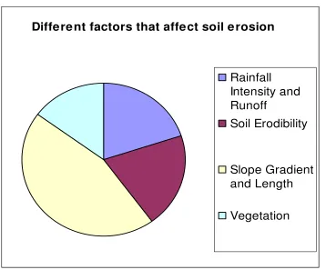
Soil erosion is the detachment and movement of soil particles by the erosive forces of wind or water. Soil detached and transported away from one location is often deposited at some other place (Wijesekera 2001). While soil erosion can be controlled, it is almost impossible to be completely stopped. Factors of soil erosion among others include rainfall intensity and runoff, soil erodibility, slope gradient and length and vegetation (fig 1.0).

Figure 1.0: Different factors that affect soil erosion

Soil erosion is one form of soil degradation along with soil compaction, low organic matter, loss of soil structure, poor internal drainage, Stalinization, and soil acidity problems (Wall et al. 2004). These other forms of soil degradation, serious in themselves, usually contribute to

Differe nt factors that affect soil e rosion

accelerated soil erosion. Soil erosion may be a slow process that continues relatively unnoticed, or it may occur at an alarming rate causing serious loss of topsoil. The loss of soil from farmland may be reflected in reduced crop production potential, lower surface water quality and damaged drainage networks.

Soil erosion in Botswana affects various aspects of the environment more specially rangeland where livestock is grazed. Traditionally, Batswana are cattle-keepers but unfortunately the idea of carrying capacity is not well understood within a large community of farmers. As a result "tragedy of the commons" scenario prevails where everybody wants to use the resources and nobody takes responsibility for their destruction and subsequent rehabilitation of the land (Totolo & Bogatsu, 2001). As the population increases, there has been a lot of pressure on land more especially around settlements. Wood resources have been significantly reduced as they are used for source of energy (firewood) by villagers. If woody vegetation is cleared, then land is left unprotected from soil erosion agents. Most of the harvesting of trees is done beyond sustainable yield and therefore recuperation of these trees is very slow. These human needs, in the long run, have a negative impact on the environment. In the meantime the process of soil erosion eats away the landscape thus reducing land available for the needs of the population. Other factors such as land clearance for agriculture, overgrazing, fire damage, use of timber for construction, poor land management and general land degradation all contribute to the overall problem. Accelerated soil erosion by water or wind may affect both agricultural areas and the natural environment, and is one of the most widespread of today's environmental problems. It has impacts which are both on-site (at the place where the soil is detached) and off-site (wherever the eroded soil ends up).

From satellite imagery, incidence of soil erosion features could be monitored throughout the whole country and after some time then statements of whether such features are increasing or not could be made. From the monitoring results, soil erosion prediction models could be used to help in the formulation of soil conservation program (Stein 2004). The main advantages of models is that they give many options under different management conditions and therefore help decision makers to adopt the best possible soil management strategy.

Soil erosion prediction models could be used to predict different soil erosion scenarios under different management conditions. Models are advantageous because a lot of time and resources are saved. For example, to predict how land will respond to specified management conditions, then you have to input parameters as required and then run the model. The results indicate the possible soil erosion scenarios from certain management conditions (Wallace 1994).

The other modern technique that could be used is Geographic Information Systems (GIS) which has the capability of overlaying several information layers and pointing out areas which are likely to suffer from soil erosion. This technique enables us to take precautionary measures, when planning, against the most sensitive areas.

2.1 BACKGROUND

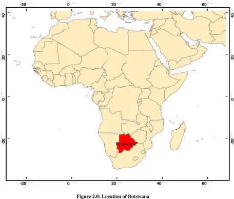
Botswana is a land-locked country dominated in geographical terms by the Kalahari Desert - a sand-filled basin averaging 1,100 metres above sea level (DSM 2000). The country lies between longitudes 200 and 300 degrees east of Greenwich and between the latitudes 180 and 270 degrees approximately south of the Equator. The country is situated in the southern African region and about two-thirds of Botswana lies within the Tropics; it is bisected by the Tropic of Capricorn (the imaginary line of latitude which is 23° 30' south of Equator).

Figure 2.0: Location of Botswana

Botswana is bordered by Zambia and Zimbabwe to the northeast, Namibia to the north and west, and South Africa to the south and southeast (figure 2). At a single point mid-stream in the Zambezi River, four countries - Botswana, Zimbabwe, Zambia and Namibia - meet. The Kalahari Desert stretches west of the eastern hardveld, covering 84% of the country. The

Kalahari extends far beyond Botswana's western borders, covering substantial parts of South Africa, Namibia and Angola.

'Desert', however, is a misnomer: its earliest travelers defined it as a 'thirstland'. Most of the Kalahari is covered with vegetation including stunted thorn and scrub bush, trees and grasslands (DOT 2001). The largely unchanging flat terrain is occasionally interrupted by gently descending valleys, sand dunes, and large numbers of pans and, in the extreme northwest, isolated hills.

In general, Botswana environmental conditions are harsh, with irregular, dramatic occurrences of droughts, floods, storms, heat and cold. Soils are of shallow depth especially along hills and slopes consisting of fine to loamy sands with considerable rock content. In valleys, along rivers and on flat land soils are deeper and fertility increases with sandy clay loams, duplex soils and black clay. Structurally these soils are relatively delicate and shallowness makes them susceptible to damage through water and wind erosion. Low humus content makes it difficult to maintain fertility and soil quality is easily exhausted if not managed in a sensitive manner.

Most of Botswana inhabitants are pastoral farmers who keep large herds of livestock and also rely on subsistence farming. This means of livelihood have put much pressure on land resources and impacted significantly on hastening soil erosion.

2.1.1 Geology of Botswana

rock. The geology of the bedrock under the Kalahari is gleaned from regional gravity and aeromagnetic surveys which cover the whole of Botswana and from drilling during mineral and water exploration programs. The oldest rocks in Botswana are Archaean in age (older than 2.5 billon years) and form part of the three major geological provinces or terrains. These are the Zimbabwe, the Limpopo Mobile Belt and Kaapvaal craton.

2.1.2 Soils

In Botswana, the legend of the soil map of the world has been adopted as the general soil classification system. It is based on measurable criteria, relatively simple and comprehensive (MOA 1990). The system is widely used internationally and therefore, forms a basis for soil correlation (comparison) with other countries with similar geophysical condition as Botswana. The original United States Development Agency (USDA), Soil Taxonomy and its subsequent editions is only used for benchmark soil profiles, but not for general mapping purposes. This system is more sophisticated, relatively more quantitative and also comprehensive. It is also widely used internationally and therefore facilitates for effective communication amongst pedologists the world over.

The Kalahari Desert stretches west of the eastern hardveld, covering 84% of the country. The desert area is mostly covered by Arenosols. The rest of the country, which is the hardveld in the east is covered by Lixisols, Leptosols, Acrisols and Regosols.

2.0.3 Vegetation

regions. Nevertheless, human activities cause some degradation or changes of vegetation types and resources and these activities and impacts influence soil erosion.

2.1.3.1 Problems and Concerns on the Use of Vegetation

Due to mismanagement and Land Tenure systems which allow for communal use of the vegetation resources the following problems are associated with vegetation (MOA 1990);

• Overgrazing due to overstocking in most of the production areas such as cattle-posts, homestead, ranching and mixed farming lands. These activities could lead to soil erosion and development of desert – like conditions (desertification or land degradation).

• As the rangelands are not protected from fire by using firebreaks and other management systems which could control and manage fire frequency and extent of burning, much of the rangelands and vegetation area subjected to burning (bushfires). These may change the density, cover, structure and the productivity of the vegetation. Animal/game habitats could change thereby, leading to changes in animal/game densities and availability.

2.1.3.2 Over-cutting, Deforestation and Over-browsing

Much of the vegetation around settlement areas, arable fields, boreholes and cattle-posts have been removed by both animals and human activities. The results of these activities are the reduction of fuelwood for the households, decline in the production of building materials (wood-based) and less browsable materials for livestock and the game.

CHAPTER 3

METHODOLOGY

3.0 INTRODUCTION

Figure 3.0: Methodology Flow Chart

In order to develop the methodology for creating GIS layers using remote sensing multi-spectral (Landsat) images, the first step was to start by creating a vegetation change layer, which is one of the factors needed to map soil erosion. Then the same methodology will be used to create other GIS layers needed in modeling soil erosion.

Images Acquisition

Study Sites Selection

Image Analyses Change Detection GIS Vegetation Change Layer Unsupervised Classification Supervised Classification Using High Resolution

Aerial Photo Images Unsupervised

Classification Using Scientific

The methodology for creating the GIS layer will be as follows;

i) Acquire Landsat/SPOT image from 1988 – 2004.

ii) Develop methodology in selected study areas.

iii) Perform Image Analysis.

iv) Develop change detection algorithms and perform change detection.

v) Create GIS Vegetation Layers.

3.0.1 Landsat/Spot Image

Satellite image data such as Landsat TM or SPOT XS have valuable characteristics due to their multi-spectral characteristics (7 bands with TM and 4 bands with SPOT), which can be used to provide a lot of quantitative information on land use and vegetation cover. On the other hand, the spatial resolution of these sensors is limited to 30m with Landsat TM and 20m with SPOT XS) which restricts their use for large scale mapping. Panchromatic (black and white) SPOT imagery has a spatial resolution of 10m, but the IRS-1 panchromatic sensor provides even higher resolution at 5.8 m (Delgadoa 2003).

Figure 4.0: Landsat TM imagery showing False Colour Band Combination

that emphasizes vegetation communities (EROS Data Centre)

SPOT imagery has a small footprint relative to MSS and TM and is good for seasonal green-up in arid-regions. Because the sensor can be pointed at areas of high interest, users can receive quicker revisit images and stereo capabilities. Spatial resolution of SPOT image is 10-meters for the panchromatic sensor 30-meters for the Multi-spectral sensor. SPOT is also priced a higher cost than Landsat TM. For this reason, SPOT images could not be acquired to be used in this project.

Figure 5.0: SPOT XS (multi-spectral), The infrared spectra emphasizes the vegetation communities (EROS Data Centre)

In this study Landsat TM were used, though if SPOT images could have been sourced, they could have enhanced the accuracy of the resultant coverage’s.

3.0.2 Image Processing

Three steps of image classification were then carried out to analyze images for different classes. All this was aimed at helping to develop change detection algorithm and perform change detection.

3.0.3 Change Detection

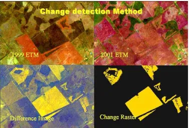
Change detection involves the comparison of images from a given location at two or more points in time. One can simply compare summaries of classifications for a given area at different points in rime or conduct a spatially explicit analysis involving direct comparisons on a pixel-by-pixel basis. Commonly used algorithms for conducting change detection include image differencing and image rationing (Singh 1986; Muchoney and Haack 1994). Bi-temporal change detection compares changes between data acquired from two discrete time periods. Trend analysis compares data across a continuous time scale. Many change detection algorithms have been developed for change detection. Some of them are Post-classification Comparison, Composite Analysis, Image Differencing, Image rationing, Change Vector Analysis etc.

Post-classification Comparison is the most commonly used method for change detection. It involves independently classifying images from two dates (usually using supervised or unsupervised classification), (Jensen, 1996). The classified images are then compared pixel by pixel to identify change. Composite Analysis technique involves placing selected bands from two images into a single dataset. The new composite dataset can then be analyzed using unsupervised classification to detect change and no-change areas. Prior knowledge of the study area is often necessary for this method since understanding the inter-relationships between classes in the composite dataset may be difficult.

Image Rationing is a simple method like image differencing. The data from two registered images are rationed pixel by pixel. Pixels that show no change will have a value of one, while pixels that changed will have a higher or lower value. Image differencing and image rationing are simple and efficient methods for detecting changes in brightness values, but the method offers no way of assessing change from one class of land-cover to another.

Change Vector Analysis this method involves determining the vector that describes both the direction and magnitude of change for each pixel between the first and second dates. Change vector analysis is able to make use of both spectral and temporal dimensions of the image data and can analyze change in all data layers, not just in selected bands.

Figure 6.0: Example of Change Detection resultant images (SLATS, 2002)

3.0.4 Accuracy Assessment

Confusion matrix is used for checking the accuracy of a classification. On the basis of a classified image and a set of regions representing test areas, a cross-tabulation of occurrence frequencies is constructed. Using confusion matrix, a number of accuracy measures can be calculated (Chips Development Team 2000).

The first step in the process is to define the relationship between test areas and pixel values in the classified image. A classification result lookup table was created during classification, this table was used to automatically establish the relationship.

Derived spectral indices for high resolution aerial photography were used to compare with scientific visualization supervised classified images. This showed areas which were wrongly classified and the accuracy of the classification.

3.1 STUDY AREA

Study Sites Area

B

C

Brisbane

Ipswitch

Beenleigh

Warwick

Beaudesert

Study

Site

Consultations were held with the Department of Environmental Protection Agency (EPA) and Natural Resources and Mines (DNRM), Queensland, to identify areas where noticeable vegetation change had occurred. This resulted in the selection of three study sites within the image that showed considerable vegetation change from year 1988 to 2004 (figure 9.0). Since the main aim of the project was to develop a methodology to map vegetation change, it was apparent to select areas where noticeable vegetation change had occurred so as to be able to see the trend of vegetation change and test whether the methodology worked.

The Greater Brisbane Region contains outstanding landscapes of great variety from the mountains to the mangroves, coastal hills and fertile valleys abutting a narrow coastal plain with a patchwork of freshwater wetlands tucked in behind ribbons of deep green estuaries. It is estimated that there are 4000 plant species (taxa) present (EPA 1999). Although there are no plants considered extinct, there are 230 that are rare or threatened of which there are 31 endangered, 68 vulnerable and 131 that are rare (Young and Dillewaard 1999). Despite dramatic changes more recently in land use and substantial loss of native vegetation, the greater Brisbane region remains a biodiversity rich part of Australia. The human settlement of Australia, since at least the late Pleistocene (more than 40 000 years ago) has reinforced the change towards sclerophyllous (Eucalypt dominated) vegetation, principally due to increases in fire frequency (Archer, et. al, 1998).

Figure 9.0: Study Area Sites Clipped Images

From the 1950’s through to the end of the 1980’s the predominant and growing land use activity for greater Brisbane was rapid urbanisation. The period 1974-1989 was characterized by rapid large scale clearance of bushland, 33% of the 1974 bushland cover on the coastal South East Queensland mainland was cleared and another 17% of the mainland part of Brisbane City had been cleared for

Site A

1988 1993 1999 2004

1988

1988

1993 1999 2004

1993 1999 2004

urbanisation in the 8 year period up to 1990. Whilst the 1980’s continued to see rapid vegetation losses there were active attempts to begin to describe the bushland values and to explore the options available to secure them for future generations (Barton 1990). The 1990’s were a period of increasing effort by governments to address community concerns about vegetation clearing. Vegetation protection laws have also been steadily improving, some councils are expanding the lands protected by their local laws. This has been reinforced by the adoption in 2000 of the Queensland Vegetation Management Act 1999 that deals with vegetation management on freehold land across all of Queensland.

3.2 DATA ANALYSIS

Analyses in this project were done within the GIS Remote Sensing environment. Data was analyzed using ERDAS Imagine 8.7 and ArcGIS 9.0. The images used in this project were for the years 1988, 1993, 1999 and 2004. All the four selected images were of the same season and same time of the year so that vegetation change could be analyzed based on the same time frame to minimise errors.

3.2.1 Data Projections

An essential step in change detection and other analysis procedures is to ensure that all data used as inputs is in the same projection. If datasets are not in the same projection they will not project to the same place on the earth and hence will not be able to be used in analysis. The datasets were acquired already geometrically corrected by Statewide Landcover and Trees Study a division within DNRM. The common projection used for this project is GDA 1994 (Geocentric Datum of Australia) and MGA Zone 56 (Map Grid of Australia).

3.2.2 Data Clipping

twelve study sites images, four for each of the three sites for the four different years, 1988, 1993, 1999 and 2004. The same coordinates were used to clip all the three sites from the four different years images so that when analysis were carried out all the images will be properly registered to each other and the cells overlay directly on each other (table 1). The process was done in ERDAS Imagine using image interpreter functions.

Site A

ULX 472250.000000 LRX 479900.000000

ULY 694305.000000 LRY 6934725.000000

Site B

ULX 491875.000000 LRX 499525.000000

ULY 6934975.000000 LRY 6926725.000000

Site C

ULX 508875.000000 LRX 516500.000000

ULY 6926775.000000 LRY 6918550.000000

3.2.3 Data Processing

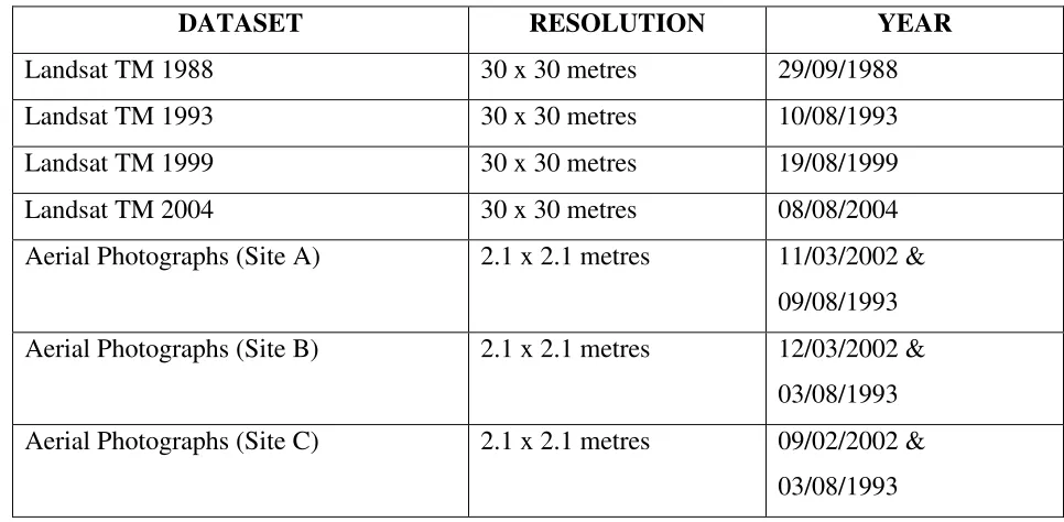
Data used in this project was obtained from the department of Natural Resources and Mines (NRM), Queensland. The data comprised of Landsat TM images for the years, 1988, 1993, 1999 and 2004. High Resolution Aerial Photographs for the study sites were also obtained from NRM (table 2). The photographs for the study sites were used to validate the Landsat TM image.

DATASET RESOLUTION YEAR

Landsat TM 1988 30 x 30 metres 29/09/1988 Landsat TM 1993 30 x 30 metres 10/08/1993 Landsat TM 1999 30 x 30 metres 19/08/1999 Landsat TM 2004 30 x 30 metres 08/08/2004 Aerial Photographs (Site A) 2.1 x 2.1 metres 11/03/2002 &

09/08/1993 Aerial Photographs (Site B) 2.1 x 2.1 metres 12/03/2002 &

03/08/1993 Aerial Photographs (Site C) 2.1 x 2.1 metres 09/02/2002 &

03/08/1993

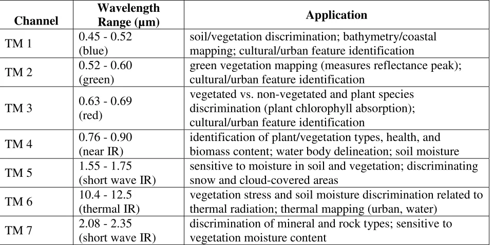
Channel

Wavelength

Range (µm) Application

TM 1 0.45 - 0.52 (blue)

soil/vegetation discrimination; bathymetry/coastal mapping; cultural/urban feature identification TM 2 0.52 - 0.60

(green)

green vegetation mapping (measures reflectance peak); cultural/urban feature identification

TM 3 0.63 - 0.69 (red)

vegetated vs. non-vegetated and plant species discrimination (plant chlorophyll absorption); cultural/urban feature identification

TM 4 0.76 - 0.90 (near IR)

identification of plant/vegetation types, health, and biomass content; water body delineation; soil moisture TM 5 1.55 - 1.75

(short wave IR)

sensitive to moisture in soil and vegetation; discriminating snow and cloud-covered areas

TM 6 10.4 - 12.5 (thermal IR)

vegetation stress and soil moisture discrimination related to thermal radiation; thermal mapping (urban, water)

TM 7 2.08 - 2.35 (short wave IR)

discrimination of mineral and rock types; sensitive to vegetation moisture content

Table 3.0: Landsat TM channel Wavelength Range (EROS 2005)

3.2.4 Classification

Classification is the process of sorting pixels into a finite number of individual classes, or categories of data based on their data file values (ERDAS Imagine, 2001). If a pixel satisfies a certain set of criteria, then the pixel is assigned to the class that corresponds to that criterion.

3.2.4.1 Unsupervised Classification

Figure 10.0: Unsupervised Classification steps using ISODATA

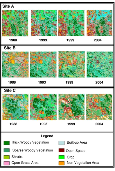
Unsupervised classification is more computer-automated. It allows the user to specify parameters that the computer uses as guidelines to distinguish different reflectance patterns in the data. With these different patterns clustered together, then different features are identified in the image. Iterative Self-Organizing Data Analysis Technique, ISODATA, algorithm was used to perform the classification. The ISODATA clustering method clusters cells reflectance pattern according to the number of classes specified within similar reflectance pattern. It is iterative in that it repeatedly performs an entire classification (outputting a thematic raster layer) and recalculates statistics (ERDAS Imagine, 2001).

The number of classes was set to eight (8). This represented the number of features in the image as could be seen through different tonal variance. Maximum Iterations was set to 24. This is the maximum number of times that the ISODATA utility recluster’s the data. It prevents this utility from running too long, or from potentially getting stuck in a cycle without reaching the convergence threshold. The conveyance threshold was set to 0.950. The convergence threshold is the maximum percentage of pixels whose cluster assignments can go unchanged between iterations. This threshold prevents the ISODATA utility from running indefinitely. 0.950 means that as soon as 95% or more

DataPrep Menu _{Select Unsupervised}

Classify Image Enter no. of classes

Enter Input and Output Enter Skip Factor

Enter Conveyance Threshold

Evaluate Classification _{Analyze individual}

of the pixels stay in the same cluster between one iteration and the next, the utility should stop processing.

Since all cells in the image were to be processed the skip factors for X and Y were set to 1. The result of the classification is shown on figure 11.0 and the detailed classification maps are shown in Appendix B.

FIGURE 11.0: Unsupervised Classification Images Results

Site A

1988 1993 1999 2004

1988

1988

1993 1999 2004

1993 1999 2004

Site C

Site B

Legend

Thick Woody Vegetation

Sparse Woody Vegetation

Shrubs

Open Grass Area

Built-up Area

Open Space

Crop

3.2.4.2 Supervised Classification (Scientific Visualisation)

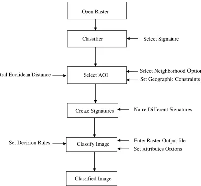
The user more closely controls supervised classification than unsupervised classification. In this process, pixels that represent recognizable patterns or those identified with help from other sources were selected. Knowledge of the data, the classes desired, and the algorithm to be used is required before selecting training samples. By identifying patterns in the imagery, the computer system is trained to identify pixels with similar characteristics. In this classification, classification was done using scientific visualization. The method uses elements of photo interpretation such as pattern colour shape etc. to aid in classification.

Figure 12.0: Supervised Classification steps using Neighborhood Options

Open Raster

Classifier Select Signature

Set Decision Rules

Select AOI

Create Signatures Name Different Signatures

Classify Image Enter Raster Output file

Set Attributes Options

Classified Image

Set Spectral Euclidean Distance Select Neighborhood Options

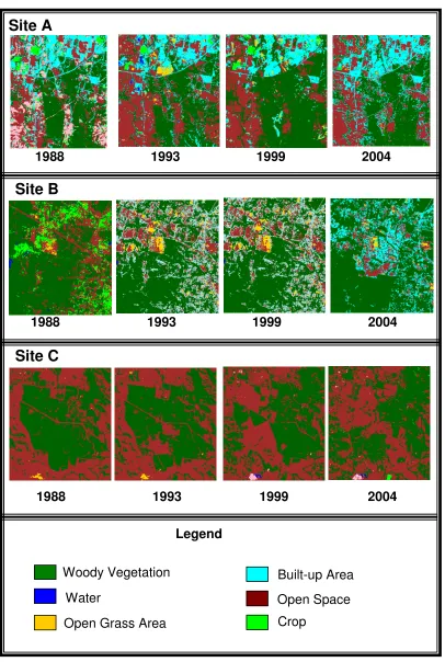
Figure 13.0: Supervised Classified Image using Scientific Visualisation

Site A

1988 1993 1999 2004

1988

1988

1993 1999 2004

1993 1999 2004

Site C

Site B

Legend

Woody Vegetation

Water

Open Grass Area

Built-up Area

Open Space

Decision rules that were used were Non Parametric Rule, selecting Feature Space option, Overlap Rule, selecting Parametric Rule option, Unclassified Rule selecting Parametric Rule option and Parametric Rule selecting Maximum Likelihood option. Decision rules help to define how the pixels will be classified. For Non Parametric Rule, Feature Space option was selected. On the Overlap Rule, the Parametric Rule option was selected. This option classifies pixels that fall into the overlap region of the classification. The pixel will be tested against the overlapping signatures only. If they don’t fall in any class then the pixel will be left unclassified (ERDAS Imagine 2001). If they fall in within any signatures, then the pixel will automatically be assigned to that signature's class. For the Unclassified Rule using Parametric Rule option, this option will classify the pixel according to the selected classes. The pixel will be tested against all of the classes’ signatures. If none of the signatures is the class signatures, the pixel will be left unclassified. With Parametric Rule using Maximum Likelihood option, classifies all pixels based on the probability that a pixel belongs to a particular class. The basic equation assumes that these probabilities are equal for all classes, and that the input bands have normal distributions (ERDAS Imagine 2001).

This method showed that it can be useful in analyzing small areas as compared to large complex areas with many different classes to be classified. The result of the classification is shown on figure 13.0 and the detailed classification maps are shown in Appendix C. The accuracy or the number of different classes that can be analyzed using this methodology depends much on the expertise of the user and his/her ability to differentiate features.

3.2.4.3 Supervised Classification (High Resolution Aerial Photography)

signature. This uses the maximum likelihood decision rule based on the probability that a pixel belongs to a particular class. The basic equation assumes that these probabilities are equal for all classes, and that the input bands have normal distributions (ERDAS Imagine 2001).

This method of classification yielded comprehensive results because training sites used for analysis were verified using aerial photographs. This method of classification helped to come as close as possible with a classified image resembling status of the area as at the time of image capture. Images from this methodology were used on the project analysis. The result of the classification is shown on figure 14.0 and the detailed classification maps are shown in Appendix D.

Figure 14.0: Supervised Classified Image (Validated with Aerial photographs)

Site A

1988 1993 1999 2004

1988

1988

1993 1999 2004

1993 1999 2004

3.2.4.5 Change Detection

Figure 15.0: Change Detection steps using ERDAS Imagine

Changes in landscapes and their components can occur in a variety of ways and at a variety of rates. Spatially, they may occur in isolation or unevenly and need to be aggregated in order to be efficiently interpreted (Blaschke T 2004). Change detection in ERDAS Imagine is useful to compute the differences between two images and to highlight changes that exceed a user-specified threshold (ERDAS Imagine, 2004).

Image Interpreter Menu

Utilities

Change Detection

Run Change Detection

Change Detection Select Change Parameters

Figure 16.0: Change Detection Using ERDAS Imagine

Site A Change

1988 _{1988-1993 1988-1999} 1988-2004

1988

1988

1988-1993 1988-1999 1988-2004

1988-1993 1988-1999 1988-2004

Site C Change

Site B Change

Legend

Change detection is applied in ERDAS Imagine through image interpreter menu. Two images of different years are entered to compute the change. These images are entered as the Before and After Image. The Before Image is the earlier of the two images whilst the After Image is the more recent of the two images. The After Image is subtracted from the Before Image to provide the image difference and Highlight Change image over time. In the output option, two files to be outputted are entered as Image Difference File and Highlight Change File. The Image Difference File (Raster Image) is the direct result of subtraction of the Before Image from the After Image. Since Change Detection calculates change in brightness values over time, the Image Difference File reflects that change using the grayscale image (ERDAS Imagine 2001). The Highlight Change Image is a five-class thematic image, typically divided into the five categories of Background, Decreased, Some Decreased, Unchanged, Some Increase, and Increased. The highlighted changes can be as percentage or value. For this project percentage output option was used. The result of the classification is shown on figure 16.0 and the detailed classification maps are shown in Appendix E.

3.2.4.6 Masking

Figure 17.0: masking steps

To be able to detect vegetation change in ERDAS Imagine all the other classes have to be masked. This operation enables one to use an image file to select (mask) specific areas from a corresponding raster file and uses those areas to create one or more new files. The areas to mask are selected by class value. All the class values of classes to be masked are set to zero or recoded to zero. When masking is executed all the zero values features are ignored. Input mask file and input file have to be the same as masking will be performed on the image area that both files have in common through intersection process. All areas were masked and the vegetation areas left so that analysis can be carried out using vegetation images.

Masking was done to select vegetation feature indices from the indices of other features. This enabled change detection to be done on vegetation only and show those areas where vegetation has changed between 1988 to 2004.

Image Interpreter Menu

Utilities

Enter output file Mask Enter input file Input mask file

CHAPTER 4

RESULTS

4.0 INTRODUCTION

The three methods of classification used namely unsupervised classification, supervised classification using scientific visualization parameters and supervised classification using aerial photographs to validate the data yielded good results. Supervised classification using aerial photographs yielded more precisely good results than the other two methods of classification. Therefore, all the analyses were done using images classified using aerial photographs.

4.1 VEGETATION MAPS

Figure 18.0: Vegetation Maps

Site A

Change

1988 1993 1999 2004

1988

1988

1993 1999 2004

1993 1999 2004

Site C

Change

Site B

Change

Legend

The above figure shows vegetation status as computed for different years with the study sites. The images were converted from raster to vector in ERDAS Imagine to create ArcInfo coverage’s to enable calculation of vegetation areas.

Figure 19.0: Raster to Vector Conversion Steps

Area m2 Hectares

Year

Vegetation Vegetation

1988 A 45979375 4597.94

1988 B 53825627 5382.56

1988 C 53750624 5375.06

1993 A 18703125 1870.31

1993 B 37563749 3756.37

1993 C 40866876 4086.69

1999 A 31776250 3177.63

1999 B 50973125 5097.31

1999 C 43331252 4333.13

2004 A 21006875 2100.69

2004 B 35586875 3558.69

2004 C 34598125 3459.81

Table 4.0: Table Showing Vegetation Areas within Study Sites

Vector Menu

Raster To Vector

Enter output vector file name Enter Image Parameters

Vector File

The maximum vegetation removed within the study sites was from between 1988 and 1993 in site A which was about 61% (table 2). That totaled approximately 2,727 hectares of removed vegetation. The area that experienced the lowest or minimum vegetation removal was between 1988 and 1993 in site B. Vegetation loss was around 15% amounting to approximately 735 hectares of vegetation loss. The years between 1993 and 1999 scored less vegetation loss when compared with vegetation loss between 1988 to 1993 and 1999 to 2004.

Year Vegetation Change

Hectares

Vegetation Percentage Change (%)

1988 – 1993 A 2825.50 61.45

1988 – 1999 A 1770.13 38.50

1988 – 2004 A 2574.38 55.99

1988 – 1993 B 1781.13 33.09

1988 – 1999 B 849.81 15.79

1988 – 2004 B 2066.50 38.39

1988 – 1993 C 1509.75 28.09

1988 – 1999 C 1560.19 29.03

1988 – 2004 C 2189.50 40.73

Table 5.0: Table Showing Vegetation Change Within Study Sites

4.2 ACCURACY ASSESSMENT (Error Matrix)

Figure 20.0: Accuracy Assessment Steps

Classifier

Accuracy Assessment

Create random points Enter reference points

Enter Images to be assessed

Accuracy assessment is a process which helps to evaluate classified images. The Accuracy Assessment CellArray is an organized way of comparing your classification with ground truth data, previously tested maps, aerial photos, or other data (ERDAS Imagine 2001).

In this project the supervised classified images using scientific visualization were assessed to see how accurately they were processed by comparing them with images which were classified using aerial photographs. The helps to show which class values were clustered wrongly, that is error matrix. The report generated also shows the accuracy of the classified image and kappa statistics. This process involves entering the image to be assessed and then generating random points, which will be used to cross tabulate with similar reference points in the image, used to assess (aerial photograph classified image).

Image Error Matrix Accuracy (%) Kappa Statistics

1988a 6 60.00 0.4444

1988b 2 86.67 0.7345

1988c 4 73.33 0.4828

1993a - 100.00 1.0000

1993b 1 93.33 0.8611

1993c 2 86.67 0.6667

1999a 1 93.33 0.8864

1999b 3 80.00 0.5455

1999c 1 93.33 0.8649

2004a - 100.00 1.0000

2004b 1 93.33 0.8214

2004c 2 86.67 0.7458

Table 6.0: Classification Accuracy Assessment Report

CHAPTER 5

DISCUSSIONS

5.1 INTRODUCTION

This chapter aims to review and discuss various issues that resulted from this project, including data accuracy and quality.

5.2 DATA PREPROCESSING

During the data-preprocessing stages, images underwent processing in order to make them usable during the classification processes conducted during this project. The processing steps that occurred during this project which require discussions are clipping, image classification and vegetation change detection.

5.2.1 Clipping

5.2.2 Image Classification

All the image classification was done in ERDAS Imagine. Two methods of Image classification were conducted in the classification of study sites, unsupervised and supervised classification. Unsupervised classification which is an automated processing procedure done by the software, was performed to get a glimpse of the features spatial arrangement in the study sites. Class features were set to eight classes. The results were pleasing though some features were aggregated with others, e.g. some areas, which were identified as water areas, were also picked as vegetation areas. However this was overcome by altering the convergence threshold.

Supervised classification was conducted using scientific visual techniques such as pattern and adjacency of features. The classification results were good. To verify the results as no field checks were conducted, classification was also conducted using high-resolution aerial photography. The results after comparing the scientific visualization classified and aerial photography classified images were quite interesting. The results accuracy ranged from 60% to 100%. It showed that no matter how classification is done, verification of results either through ground truthing and use of high-resolution photography is crucial and cannot be compromised.

All the images were acquired rectified for any distortions, e.g. geo-rectified, contrast etc. from DNRM. The high-resolution imagery used to verify the classification was geo-referenced so that it could be overlaid with the images. When classifying the images, vegetation comprised of woody vegetation, sparse vegetation and shrubs. This was maintained like that because the essence of the study is to develop vegetation cover maps, which may be used to model soil erosion. However, doing some sites visits and picking vegetation species can further classify the vegetation composition. Using SPOT images can also enhance accuracy. In this project SPOT images could have been used if they were readily available.

5.2.3 Change Detection

CHAPTER 6

CONCLUSIONS AND RECOMMENDATIONS

6.0 CONCLUSIONS

The initial main aim of this project was to model soil erosion risk areas in Botswana. Since modeling involves the use of different accurate data sets, datasets in Botswana were old and comprised of digital maps which were compiled in 1988 a small scale ranging from 1:1,000,000 and 1:1,500,000. Despite the fact that datasets were old, also there was no time series datasets that could be used to model trend. This necessitated the need to use remote sensing multi-spectral data for creating GIS vegetation change layers.

Remote sensing multi-spectral data can be used to generate datasets that can be used in mapping soil erosion risk areas. Remote Sensing data has been used in a number of applications to develop accurate and near real time datasets for different scenarios. This led to this project looking into developing a methodology that will help in developing datasets to be used in soil erosion risk areas mapping. Though the project used the development of vegetation change datasets, it should be clear that the methodology would aid in development of other relevant datasets to enable modeling of soil erosion risk areas. The methodology might undergo some changes for the development of other datasets since different datasets require different parameters.

The accuracy of the datasets is acceptable because the verification for the classified featured was done using high-resolution aerial photography. This data can be further improved by doing some ground truth to establish the species of different vegetation stratus in the study sites.

6.1 RECOMMENDATIONS

This project main thrust was to develop a methodology for creating vegetation GIS layer, which is one of the key factors in soil erosion. This was achieved and methodology is subject to modification to suit the development of other datasets, which can be used in soil erosion mapping.

6.1.1 Further Work

Once all the relevant datasets have been generated, the Digital Elevation Model for the area where soil erosion risk areas are to be mapped can be obtained and used to aid in analysis. Terrain is one of factors, which influence soil erosion, and the DEM will help to use aspect to identify prone areas.

References

Armstron, J., Danaher, T., Goulevitch, B. and Byrne, M. 2002. Geometric correction of Landsat TM and ETM+ for mapping woody vegetation cover and change detection over Queensland. Proceedings 11th Australian Remote Sensing and Photogrammetry Conference, Brisbane.

Barton, A 1990, ‘Environmental History Literature Review’, viewed 06 April 2005, <http://urbac.wildlife.org.au/sop/env_his_lit_rev.pdf>

Blaschke, T 2004, Towards a Framework for Change Detection Based on Image Objects, Centre for Geoinformatics University of Salzburg Hellbrunner Str. 34, A-5020 Salzburg.

Boschetti, L., Flasse, S., Trigg, S., Brivio, P.A. and Maggi, M., 2001, A methodology for the

validation of low resolution remotely sensed data products, accepted for Proceedings of the 4th AITA Conference (Rimini, Italy, 9-12 October 2001).

Chips Development Team 2000, Creating a Confusion Matrix, viewed 28 May 2005 <http://www.geogr.ku.dk/chips/Manual/f168.htm>

Confusion Matrix, viewed 28 May 2005

<http://www2.cs.uregina.ca/~hamilton/courses/831/notes/confusion_matrix/confusion_matrix.html> Danaher, T Armston, J and Collett, L 2004, A Regression Model Approach for Mapping Woody Foliage Projective Cover Using Landsat Imagery in Queensland, Australia.

Department of Surveys and Mapping (DSM), 2000, ‘Botswana National Atlas’, viewed 16 April 2005,< http://www.atlas.gov.bw>

Department of Tourism (DoT), 2001, ‘Botswana Geographical Information’, viewed 16 April 2005, <http://www.botswana-tourism.gov.bw/tourism/geographical/geographical.html>

Donkor, S.M.K. 1995. Land Conservation and Rehabilitation in Botswana. Final Report. Ministry of Agriculture, Gaborone. Botswana.

Delgadoa J, Soares, A, Carvalho, J 2003, Landsat-Spot Digital Images Integration Using Geostatistical Cosimulation Techniques, 1049-001 Lisbon, Portugal EROS Data Center 2002,

LANDSAT TM , viewed 27 May 2005, <http://edcwww.cr.usgs.gov/webglis> ERDAS Imagine V8.5, 2001, Tour Guides, ERDAS Inc., Atlanta, Georgia

Goulevitch, B.M., Danaher, T.J., Stewart, A.J., Harris, D.P., and Lawrence, L.J. 2002,

Jensen, JR 1996, Introductory Image Processing, A Remote Sensing Perspective, Prentice Hall Inc, New Jersey , pg. 257-279

J.B. Collins and C.E. Woodcock, “An assessment of Several Linear Change Detection Techniques for Mapping Forest Mortality Using Multitemporal Landsat TM Data”, Remote Sensing of

Environment, Vol. 56, No 1, pp. 66-67, January 19996.

Mather, PM, Tso, B 2001, Classification Methods for Remotely Sensed Data, Taylor & Francis Inc. London

Otlogetswe Totolo, O, Bogatsu, YG, 2001, ‘How do we minimise soil erosion and its environmental impact?’, viewed 12 May 2005, <http://www.lethbridgecollege.ab.ca/dept/IEM/case.htm>

Pratt, WK 2001, Digital Image Processing, John Wiley & Sons Inc. New York

Procedures and Considerations for Conducting Digital Change Detection, viewed 28 May 2005 <http://www.personal.psu.edu/users/j/b/jbs191/steps.htm>

Queensland Department of Natural Resources and Mines, 2005, Land Cover Change in Queensland, viewed 25 May 2005 <http://www.nrm.qld.gov.au/slats>

Stein, A, Freek van der Meer, Gorte, B 1999, Spatial Statistics for Remote Sensing Kluwer Academic Publishers London

Stein, A, Freek van der Meer, Gorte, B 2004, Remote Sensing Image analysis, Kluwer Academic Publishers London

Sunstrum, M, 2000, Case Study - Environmental Impact of Fuelwood Use in Botswana, viewed 12 May 2005, <http://www.lethbridgecollege.ab.ca/dept/IEM/case.htm>

Wallace, J, Furby, S 1994, Detecting and Monitoring Changes in Land Condition Through Time using Remotely Sensed Data, viewed 24 May 2005,

<http://www.cmis.csiro.au/rsm/research/remveg/vegassess.html>

Appendix A

Appendix A

1.0

Introduction

The University of Southern Queensland Faculty of Engineering and Surveying

ENG4111/2 Research Project

PROJECT SPECIFICATION

FOR: Mr. David Stimela

TOPIC: Developing a Methodology Using Multi-spectral Remote Sensing Data for Mapping Vegetation Change – A Key Variable in Soil Erosion Mapping

SUPERVISOR: Dr Sunil Bhaskaran PROJECT AIMS:

1. To develop a project design (conceptual and logical) for creating a database of vegetation related spatial and temporal variables in a Geographic Information System (GIS) environment.

2. To study the different existing and available datasets and document their limitations with regard to data standards and accuracy in detail, and list datasets to be freshly acquired. 3. To develop a methodology to model detect vegetation change related data and to perform

spatial and digital image analysis using customised softwares for developing interactive maps showing areas affected by different degrees of vegetation change within and around Brisbane metropolitan area.

PROGRAMME: Issue B, 20 March 2005

1. Prepare draft proposal (3-4) with abstract, introduction and literature review (Harvard referencing system), methodology study area, data sources, availability, copy rights, data analysis, and anticipated results and a clear and practical project time line (Submit, 16th May 2005).

2. Develop procedures and steps – Conceptual and logical design for developing the information system database design (Submit by end June, 2005).

3. Build the database for modelling vegetation change and document limitations (Submit by mid July, 2005)

4. Spatial and Image Analysis and final output (Submit by end June, 2005). 5. Start writing dissertation by August, 2005. First Draft in to supervisor by 16

September, 2005.

6. Submit final dissertation by 27 October 2005. AGREED:

Appendix B

Appendix B

1.0

Introduction

Appendix C

Appendix C

1.0

Introduction

Appendix D

Appendix D

1.0

Introduction