Detecting the position of non-linear component in periodic structures from the system responses to dual sinusoidal excitations

promoting access to White Rose research papers

Universities of Leeds, Sheffield and York

http://eprints.whiterose.ac.uk/

This is an author produced version of a paper published in International Journal of Non-Linear Mechanics.

White Rose Research Online URL for this paper: http://eprints.whiterose.ac.uk/3583/

Published paper

Detecting the Position of Nonlinear Component in

Periodic Structures from the System Responses to

Dual Sinusoidal Excitations

Z.K. Peng, Z.Q. Lang

Department of Automatic Control and Systems Engineering, University of Sheffield Mappin Street, Sheffield, S1 3JD, UK

Email: [email protected]; [email protected]

Abstract: Based on the Nonlinear Output Frequency Response Functions (NOFRFs), a novel method is developed to detect the position of nonlinear components in periodic structures. The detection procedure requires exciting the nonlinear systems twice using two sinusoidal inputs separately. The frequencies of the two inputs are different; one frequency is twice as high as the other one. The validity of this method is demonstrated by numerical studies. Since the position of a nonlinear component often corresponds to the location of defect in periodic structures, this new method is of great practical significance in fault diagnosis for mechanical and structural systems.

1 Introduction

Periodic structures are defined as structures consisting of identical substructures connected to each other in identical manner. The real life systems which can be modelled as either finite or infinite, one-dimension or multi-dimension periodic structures range from the simple structures like periodically supported beams [1]~[6], plates[5][6] and building block [7]. Analysis of the free and forced vibration and the mode analysis of linear periodic structures are of particular interests [1]-[6]. Mead [8] provides an excellent review about periodic structure studies.

Attentions also have been paid to the study of nonlinear periodic structures [9]-[13]. Chi and Rosenberg [9] have studied the existence of classical normal mode motion in one-dimension non-linear mass-spring-damper systems with many degrees of freedom where all springs and / or all dampers may be strongly non-linear. Using exact and asymptotic techniques, Vakakis et al [10] have studied the localized responses of a nonlinear

semi-analytical framework for the study of mechanical systems with local nonlinearities has been presented. Chakraborty and Mallik [12] have investigated the harmonic vibration propagation in an infinite, non-linear periodic chain using a perturbation approach where the case of cyclic one-dimension nonlinear chain has also been discussed. Marathe and Chatterjee [13] have studied the Wave attenuation in one-dimension nonlinear periodic structures using harmonic balance and multiple scale method. In engineering practices, there are considerable periodic structures that behave nonlinearly just because one or a few components have nonlinear properties, and the nonlinear component is often the component where a fault or abnormal condition occurs. One of the well known examples is beam structures [14] with breathing cracks, the global nonlinear behaviors of which are caused only by a few cracked elements. Therefore it is of great significance to effectively detect the position of the nonlinear component in a periodic structure. The detection of damage in large periodic structures has been studied by Zhu and Wu [15]. In their studies, the periodic structure with damage is still considered to be linear and the locations and magnitude of damage in large mono-coupled periodic systems have been estimated using measured changes in the natural frequencies. Based on a one-dimensional periodic structure model, Sakellariou and Fassois [7][16] have used a stochastic output error vibration-based methodology to detect the damage in structures where the damage elements were modeled as components of cubic stiffness.

In this paper, a novel method is derived based on the NOFRF concept to detect the position of the nonlinear component in a periodic structure. The detection procedure requires exciting the nonlinear systems twice using two sinusoidal inputs separately. The frequencies of the two inputs are required to be different; one frequency is twice as high as the other one. Numerical studies verify the effectiveness of the method. The new method is of great practical significance in fault diagnosis for mechanical and structural systems.

The paper is organized as follows. Section 2 gives a brief introduction to the new concept of NOFRFs. Some important properties of the NOFRFs for locally nonlinear MDOF systems, which were first revealed in the authors’ recent studies [23], are introduced in Section 3. The novel method for the nonlinear component position detection is presented in Section 4. In Section 5, three numerical case studies are used to verify the effectiveness of the proposed method. Finally conclusions are given in Section 6.

2. Output Frequency Response Functions of Nonlinear Systems

2.1 Output Frequency Response Functions under General Input

The definition of NOFRFs is based on the Volterra series theory of nonlinear systems. The Volterra series extends the well-known convolution integral description for linear systems to a series of multi-dimensional convolution integrals, which can be used to represent a wide class of nonlinear systems [18].

Consider the class of nonlinear systems which are stable at zero equilibrium and which can be described in the neighbourhood of the equilibrium by the Volterra series

i n

i

i n

N

n

n u t d

h t

x( ) (τ ,...,τ ) ( τ ) τ

1 1

1

∏

∑∫ ∫

= =

∞

∞ −

∞

∞

− −

= _L (1)

where x(t) and u(t) are the output and input of the system, h_n(τ₁,...,τ_n) is the nth order

Volterra kernel, and N denotes the order of the Volterra series representation. Lang and

Billings [18] derived an expression for the output frequency response of this class of nonlinear systems to a general input. The result is

⎪ ⎪ ⎩ ⎪ ⎪ ⎨ ⎧

=

∀ =

∫

∏

∑

= +

+ =

− =

ω ω ω

ω σ ω ω

ω π

ω

ω ω

ω

n

n n

i

i n

n n

n

N

n n

d j U j

j H n

j X

j X j

X

,..., 1

1 1

1

1

) ( ) ,..., ( )

2 (

1 ) (

) ( )

( for

This expression reveals how nonlinear mechanisms operate on the input spectra to produce the system output frequency response. In (2), X(jω) is the spectrum of the system output, X_n(jω) represents the nth order output frequency response of the system,

n j

n n

n

n j j h e d d

H ( ω ,..., ω ) ... (τ ,...,τ ) ωτ ωnτn τ ... τ

1 ) ,..., ( 1

1 11

+ + − ∞

∞ − ∞

∞ −

∫

∫

= (3)

is the nth order Generalised Frequency Response Function (GFRF) [18], and

∫

∏

= +

+ ω ω =

ω

ω σ ω ω

ω

n

n n

i

i n

n j j U j d

H

,..., 1

1

1

) ( ) ,..., (

denotes the integration of

∏

n

i

i n

n j j U j

H

1

1,..., ) ( )

( ω ω ω

ω ω

ω₁+_L+ _n = . Equation (2) is a natural extension of the well-known linear relationship )

( ) ( )

(jω H jωU jω

X = , where H(jω) is the frequency response function, to the

nonlinear case.

For linear systems, the possible output frequencies are the same as the frequencies in the input. For nonlinear systems described by equation (1), however, the relationship between the input and output frequencies is more complicated. Given the frequency range of an input, the output frequencies of system (1) can be determined using the explicit expression derived by Lang and Billings in [18][24].

Based on the above results for the output frequency response of nonlinear systems, a new concept known as the Nonlinear Output Frequency Response Function (NOFRF) was recently introduced by Lang and Billings [22]. The NOFRF is defined as

∫ ∏

∫

∏

= + + = =

+

+ =

=

ω ω ω

ω ω

ω ω

ω

σ ω

σ ω ω

ω ω

n n

n n

i

i

n n

i

i n

n

n

d j U

d j U j

j H

j G

,..., 1

,..., 1

1

1 1

) (

) ( ) ,..., (

)

( (4)

under the condition that

0 )

( )

2 (

1 ) (

,..., 1

1 1

≠

=

∫ ∏

= + + = −

ω ω ω

ω σ ω π

ω

n

n n

i

i n

n U j d

n j

U (5)

Notice that G_n(jω) is valid over the frequency range of U_n(jω) , which can be

determined using the algorithm in [18].

By introducing the NOFRFs G_n(jω), n=1,_LN, equation (2) can be written as

∑

∑

= =

=

= N

n

n n

N

n

n j G j U j

X j

X

1 1

) ( ) ( )

( )

( ω ω ω ω (6)

output frequency response behaviour. It can be seen from equation (4) that G_n(jω) depends not only on H_n (n=1,…,N) but also on the input U(jω). For any structure, the

dynamical properties are determined by the GFRFs (n= 1,…,N). But, according to

equation (4), the NOFRF

n

H

) (jω

G_n is a weighted sum of Hn(jω1,..., jωn) over ω

ω

ω₁+_L+ _n = with the weights depending on the test input. Therefore G_n(jω) can be used as an alternative representation of the dynamical properties described by . The most important property of the NOFRF

n

H

) (jω

G_n is that it is one dimensional, and thus

allows the analysis of nonlinear systems to be implemented in a convenient manner similar to the analysis of linear systems. Moreover, there is an effective algorithm [22] available which allows the estimation of the NOFRFs to be implemented directly using system input output data.

2.2 Output Frequency Response Functions under Harmonic Inputs When system (1) is subject to a harmonic input

) cos(

)

(t = A ω t+β

u _F (7)

Lang and Billings [18] showed that equation (2) can be expressed as

∑

∑

∑

= + + =

= ⎟

⎟ ⎠ ⎞ ⎜

⎜ ⎝ ⎛ =

= N

n

k k

k k

n n

N

n n

kn k

n n A j A j

j j

H j

X j

X

1

1 ₁ 1 1

) ( ) ( ) , , ( 2

1 )

( )

(

ω ω ω

ω ω

ω ω

ω ω

L

L

L (8)

where

⎩ ⎨ ⎧ =

0 | | ) (

) ( sign β

ω_k A ej k

j A

i

if

{

}

otherwise

, , 1 , 1

,k i n

k _F

ki ∈ ω =± = L ω

(9)

Define the frequency components of nth order output of the system as . Then

according to equation (8), the frequency components in the system output can be expressed as

n Ω

U

1

=

Ω =

Ω (10)

and Ω_n is determined by the set of frequencies

{

}

i

n | , 1, ,

1+L+ =± = L

=ω ω ω ω

ω (11) From equation (11), it is known that if all

n

k

k ω

ω₁,_L, are taken as −ωF, then ω=−nωF. If k of these are taken as ω_F, then ω =(−n+2k)ω_F. The maximal k is n. Therefore the

possible frequency components of X_n(jω) are

n

Ω =

{

}

Moreover, it is easy to deduce that

} , , 1 , 0 , 1 , , ,

{

1

N N

k

k _F

N

n

n L L

U

Ω

=

Equation (13) explains why superharmonic components are generated when a nonlinear system is subjected to a harmonic excitation. In the following, only those components with positive frequencies will be considered.

The NOFRFs defined in equation (4) can be extended to the case of harmonic inputs [25] as

∑

∑

( (n = 1,…, N ) (14)

under the condition that

0 ) ( ) ( 2 1 ) ( 1 1 ≠ =

∑

n j A j A j

A

L

L (15)

Obviously, is only valid over GnH(jω) Ωn defined by equation (12). Consequently, the output spectrum X(jω) of nonlinear systems under a harmonic input can be expressed as

∑

∑

n j G j A j

X j X 1 1 ) ( ) ( ) ( )

( ω ω ω ω (16)

When k of the n frequencies of

n

k

k ω

ω , ,

1 L are taken as ωF and the remainders are as

F ω

− , substituting equation (9) into equation (15) yields,

β

ω _{| |} ( 2 )

2 1 ) ) 2 (

( k j n k

n n n F

n j n k A C e

A − + = − + (17)

Moreover β β ω ω ω ω ω ) 2 ( ) 2 ( | | 2 1 | | ) , , , , , ( 2 1 ) ) 2 ( ( k n j k n n n k n j k n n k n F F k F F n n F H n e C A e C A j j j j H k n j G + − + − − − − = + − 4 4 8 4 4 7 6 L 4 48 4 47 6 L ) , , , , ,

(6474_L484 64 74_L4 84

k n F F k F F

n j j j j

H

−

− −

= ω ω ω ω (18) where H_n(jω₁,...,jω_n) is assumed to be a symmetric function. Therefore, in this case,

over the nth order output frequency range

) (jω

G_nH Ω_n=

{

}

equal to the GFRFH_n(jω₁,...,jω_n) evaluated atω1 =L=ωk =ωF, ωk+1 =L=ωn =−ωF, .

n k=0,_L,

Substituting equations (17) and (18) into (16), it can be derived that the output spectrum )

(jω

Y of nonlinear systems subjected to a harmonic input can be expressed as

[ ]

∑

= + − + −

= ( 1)/2 1 ) 1 ( 2 ) 1 (

2 ( ) ( )

) ( k N n F n k F H n k

F G jk A jk

jk

X ω ω ω (k =0,1,_L,N) (19)

3. NOFRFs of Nonlinear Periodic Structures

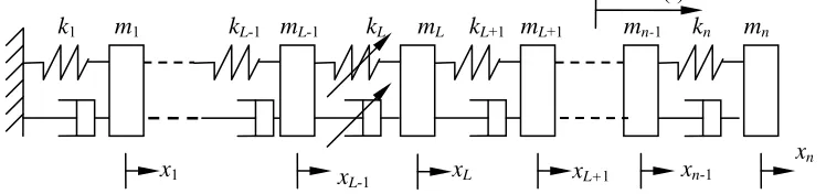
Consider the one-dimension nonlinear periodic structures where the Lth component is

nonlinear, which have be used in [7], [12], [13] and [15], shown in Figure 1.

mn

kn

mn-1

mL-1

m1 kL-1

k1

x1 _xL-1 xn-1

xn

u(t) mL+1

kL+1

mL

kL

xL xL+1

Figure 1, a locally nonlinear multi-degree freedom oscillator

Assume the restoring forces S_LS(Δ) and of the Lth spring and damper are the

polynomial functions of the deformation Δ and ) (Δ& LD

S

Δ& respectively, e.g.,

∑

( ,

∑

(& &

where P is the degree of the polynomial. Without loss of generality, further assume

. Denote

n L≠1,

∑

∑

i x x r x x

w NonF

2 1 2

1 ) ( )

(_{& &} (21)

}2 } '

0 0 0

0 _⎟⎟

⎠ ⎞ ⎜ ⎜ ⎝ ⎛ − = −

− n L

L

NonF NonF

NF _{L L} (22)

Then the motion of the nonlinear oscillator in Figure 1 is described in a matrix form as. ) (t F NF Kx x C x

M&&+ &+ =− + (23)

where M is the system mass matrix,

⎥ ⎥ ⎥ ⎥ ⎦ ⎤ ⎢ ⎢ ⎢ ⎢ ⎣ ⎡ = n m m m M L M O M M L L 0 0 0 0 0 0 2 1 and ⎥ ⎥ ⎥ ⎥ ⎥ ⎥ ⎦ ⎤ ⎢ ⎢ ⎢ ⎢ ⎢ ⎢ ⎣ ⎡ − − + − − + − − + = − − n n n n n n c c c c c c c c c c c c c C 0 0 0 0 0 0 1 1 3 3 2 2 2 2 1 L O M O O O M O L ⎥ ⎥ ⎥ ⎥ ⎥ ⎥ ⎦ ⎤ ⎢ ⎢ ⎢ ⎢ ⎢ ⎢ ⎣ ⎡ − − + − − + − − + = − − n n n n n n k k k k k k k k k k k k k K 0 0 0 0 0 0 1 1 3 3 2 2 2 2 1 L O M O O O M O L

are the system mass, damping and stiffness matrix respectively. is the displacement vector, and

'

1, , )

(x x_n

' 1 ) 0 , , 0 ), ( , 0 , , 0 ( )

( 67_L8 67_L8 J n J t u t F − −

= (24) is the external force vector acting on the Jth mass of the oscillator.

The system described by equation (23) is a typical locally nonlinear periodic structure. The Lth nonlinear component can lead the whole system to behave nonlinearly. In this

case, the Volterra series can be used to describe the relationships between the displacements x_i(t) (i=1,_L,n) and the input force u(t) as below

(25) Z j Z Z N j j j i

i t h u t d

x ( ) (τ ,...,τ ) ( τ ) τ 1 1 1 ) , (

∏

∑∫ ∫

where h_(i,j)(τ₁,...,τ_j) is the jth order Volterra kernel associated to the ith mass. In the

frequency domain, the relationship (16) can be expressed as

∑

∑

i j X j G j U j

X

1 (,) 1 (,)

) ( ) ( ) ( )

( ω ω ω ω (i=1,_L,n) (26) where )G_(i,l)(jω is the lth order NOFRF associated to the ith mass.

Without loss of generality, assume L<J, as revealed in [23], for any two consecutive masses,

the NOFRFs of system (23) satisfy following relationships

) ( ) ( ) ( ) ( ) ( ) ( ) , 1 ( ) , ( 1 , ) 2 , 1 ( ) 2 , ( 1 , 2 _ω ω ω λ ω ω ω λ j G j G j j G j G j N i N i i i N i i i i + + + + _{= = = =} L

(1≤i≤n−1) (27)

) ( ) ( ) ( ) ( ) ( )

( , 1

) , 1 ( ) , ( ) 1 , 1 ( ) 1 , ( 1 ,

1 _ω λ ω

ω ω ω ω λ j j G j G j G j G

j iZi

Z i Z i i i i i + + + + _{= = =}

(1≤i≤L−2 or J ≤i≤n−1; 2≤Z ≤N) (28)

) ( ) ( ) ( ) ( ) ( )

( , 1

) , 1 ( ) , ( ) 1 , 1 ( ) 1 , ( 1 ,

1 _ω λ ω

ω ω ω ω λ j j G j G j G j G

j i_Zi

Z i Z i i i i i + + + + _{= ≠ =}

(L−1≤i≤J−1,2≤Z ≤N) (29)

Based on these relationships of the NOFRFs, a novel method can be developed to determine the position of the nonlinear element in system (23).

As equations (27)~(29) are the basis of this study, but the derivation and justification of these equations can take quite a lot of contents and, therefore, the elaboration of them are not given in this paper. However, for the sake of completion, a numerical case is given here to justify equations (27)~(29). The numerical case study is conducted on a damped 8-DOF oscillator whose fourth spring (L = 4) was nonlinear. As widely used in

modal analysis, the damping was assumed to be proportional to the stiffness, e.g., C=μK .

The values of the system parameters are taken as 1

8

1 = =m =

m _L , r₁ =k₁ =_L=k₈ =3.5531×104, μ=0.01 2

8 . 0 r

and the input was a harmonic force acting on the 6th mass (J = 6), u(t)=Asin(2π×20t).

If only the NOFRFs up to the 4th order is considered, according to equations (16) and (17), the frequency components of the outputs of the 8 masses can be written as

) ( ) ( ) ( ) ( )

( (,1) 1 (,3) F 3 F H i F F H i F

i j G j U j G j U j

X ω = ω ω + ω ω

) 2 ( ) 2 ( ) 2 ( ) 2 ( ) 2

( (,2) 2 (,4) F 4 F H i F F H i F

i j G j U j G j U j

X ω = ω ω + ω ω

( 3 ) (,3)( 3 F) 3( 3 F)

H i F

i j G j U j

X ω = ω ω

) 4 ( ) 4 ( ) 4

( (,4) F 4 F H

i F

i j G j U j

X ω = ω ω (i=1,L,8) (30)

From equation (30), it can be seen that, using the method in [22], two different inputs with the same waveform but different strengths are sufficient to estimate the NOFRFs up to 4th order. Therefore, in this numerical study, two different inputs are used with A=0.8 and A=1.0 respectively. The simulation studies were conducted using a fourth-order Runge-Kutta method to obtain the forced response of the system.

The evaluated results of , , and for all masses are given in Table 1. According to relationships (27)~(29), it is known that the following relationships should be tenable.

) (

1 F

H

j

G ω ₃ ( F)

H

j

G ω G₂H(j2ω_F) G₄H(j2ω_F)

) ( ) ( ) ( ) ( ) ( )

( , 1

3 ) 3 , 1 ( ) 3 , ( ) 1 , 1 ( ) 1 , ( 1 , 1 F i i F H i F H i F H i F H i F i i j j G j G j G j G

j λ ω

ω ω ω ω ω λ + + +

+ _{= = = for =1,2,6,7}

i ) ( ) ( ) ( ) ( ) ( )

( , 1

3 ) 3 , 1 ( ) 3 , ( ) 1 , 1 ( ) 1 , ( 1 , 1 F i i F H i F H i F H i F H i F i i j j G j G j G j G

j λ ω

ω ω ω ω ω λ + + +

+ _{= ≠ = for =3,4,5}

i ) 2 ( ) 2 ( ) 2 ( ) 2 ( ) 2 ( ) 2

( , 1

4 ) 4 , 1 ( ) 4 , ( ) 2 , 1 ( ) 2 , ( 1 , 2 F i i F H i F H i F H i F H i F i i j j G j G j G j G

j λ ω

ω ω ω ω ω λ + + +

+ _{= = = for 1, ,7} L =

i

(31) Table 1. The evaluated results of ₁H( _F), and

j

G ω ₃ ( F)

H

j

G ω G₂H(j2ω_F) 4 ( 2 F) H j G ω ) ( 1 F H j G ω

(×10-6)

) ( 3 F H j G ω

(×10-9)

) 2 ( 2 F H j G ω

(×10-9)

) 2 ( 4 F H j G ω

(×10-10)

Mass 1 -1.9442+2.8776i 5.4586-7.3663i 6.0215-12.9855i -1.9521-3.4108i

Mass 2 -4.1766+4.8383i 11.5721-12.2812i 18.5089-19.1412i -1.3474-7.1855i

Mass 3 -6.7369+5.061i 18.3492-12.5736i 38.1986-9.3255i 3.9767-10.0350i

Mass 4 -9.2319+2.952i -12.7969+5.4557i -38.0890+6.2165i -4.6556+9.5167i

Mass 5 -10.7758-1.6643i -5.4352+7.5922i -16.5271+16.8545i 1.1500+6.3785i

Mass 6 -10.1014-8.3275i 1.2207+7.2432i -1.2526+13.2872i 2.7770+2.3907i

Mass 7 -15.1122-0.8377i 6.0974+5.9104i 6.2132+5.7292i 2.2699-0.4817i

Table 2, the evaluated values of , 1( ), and 1 F i i jω λ + ) ( 1 , 3 F i i jω

λ + , 1_{( 2 )}

2 F

i i

j ω

λ + , 1_{( 2 )}

4 F i i j ω λ + ) ( 1 , 1 F i i jω

λ + , 1_{( )}

3 F

i i

jω

λ + , 1_{( 2 )}

2 F

i i

j ω

λ + , 1_{( 2 )}

4 F

i i

j ω

λ +

i=1 0.5396-0.0639i 0.5396-0.0639i 0.5078-0.1764i 0.5078-0.1765i

i=2 0.7412-0.1614i 0.7412-0.1614i 0.5727-0.3613i 0.5729-0.3613i

i=3 0.8211-0.2856i -1.5678 +0.3142i -1.0158+0.0791i -1.0158+0.0791i

i=4 0.7955-0.3968i 1.2730+0.7743i 1.3178+0.9677i 1.3176+0.9674i

i=5 0.7160-0.4255i 0.8963+0.9014i 1.3735+1.1144i 1.3735+1.1145i

i=6 0.6969+0.5124i 0.6969+0.5124i 0.9568+1.2563i 0.9568+1.2562i

i=7 0.8277+0.2166i 0.8277+0.2166i 0.7570+0.6108i 0.7570+0.6108i

From the NOFRFs in Table 1, , , and

( ) can be evaluated, and the results are given in Tables 2. The results shown in Tables 2 have a strict accordance with the relationships in (31). Therefore, the numerical study verifies relationships (27)~(29).

) ( 1 , 1 F i i jω

λ + , 1_{( )}

3 F

i i

jω

λ + , 1_{( 2 )}

2 F

i i

j ω

λ + , 1_{( 2 )}

4 F i i j ω λ + 7 , , 1_L = i

4. The Nonlinear Component Position Detection Method

When the input u(t) is a sinusoidal type force of frequency ωF , according to the definition of NOFRFs under a harmonic input in Section 2.2, it is known from equations (27)~(29), that ) ( ) ( ) ( ) ( ) ( ) ( )

( _{, 1}

) 1 2 , 1 ( ) 1 2 , ( ) 3 , 1 ( ) 3 , ( ) 1 , 1 ( ) 1 , ( F i i F D i F D i F i F i F i F i j j G j G j G j G j G j G ω λ ω ω ω ω ω ω ₊ + + + + + = = = =

= _{L L}

(D=1,2,_L) (1≤i≤L−2 or J ≤i≤n−1) (32)

) ( ) ( ) ( ) ( ) ( ) ( )

( _{, 1}

) 1 2 , 1 ( ) 1 2 , ( ) 3 , 1 ( ) 3 , ( ) 1 , 1 ( ) 1 , ( F i i F D i F D i F i F i F i F i j j G j G j G j G j G j G ω λ ω ω ω ω ω ω ₊ + + + + + = = = =

≠ _{L L}

(D=1,2,_L) (L−1≤i≤J−1) (33)

) 2 ( ) 2 ( ) 2 ( ) 2 ( ) 2 ( ) 2 ( ) 2

( _{, 1}

) 2 , 1 ( ) 2 , ( ) 4 , 1 ( ) 4 , ( ) 2 , 1 ( ) 2 , ( F i i D i D i F i F i F i F i j j G j G j G j G j G j G ω λ ω ω ω ω ω ω ₊ + + + = = = =

= _{L L}

) 3 ( ) 3 ( ) 3 ( ) 3 ( ) 3 ( ) 3 ( ) 3

( _{, 1}

) 1 2 , 1 ( ) 1 2 , ( ) 5 , 1 ( ) 5 , ( ) 3 , 1 ( ) 3 , ( F i i F D i F D i F i F i F i F i j j G j G j G j G j G j G ω λ ω ω ω ω ω ω ₊ + + + + + = = = =

= _{L L}

M (D=1,2,_L) (i=1,_L,n−1) (34)

According to equation (19), the first harmonic components of ( ) can be written as

) (t

xi i=1,L,n

[ ]

∑

= − −

= /2 1 1 2 ) 1 2 , ( ( ) ( ) ) ( N k F k F H k i F

i j G j A j

For the masses which are on the left of the nonlinear spring or on the right of the input force, substituting equation (32) into (35) yields

[ ] ) ( ) ( ) ( ) ( ) ( )

( /2 , 1 ₁

1 1 2 ) 1 2 , 1 ( 1 , F i F i i N k F k F H k i F i i F

i j j G j A j j X j

X ω λ ω ω ω λ + ω ₊ ω

= + − −

+ ₌

=

∑

(1≤i≤L−2 or J ≤i≤n−1) (36)

Therefore, ) ( ) ( ) ( 1 1 , F i F i F i i j X j X j ω ω ω λ +

+ _{= (1≤ ≤ −2}

L

i or J ≤i≤n−1) (37)

For the masses located between the nonlinear spring and the input force, substituting equation (33) into (35) yields,

[ ] [ ] ) ( ) ( ) ( ) ( ) ( ) ( ) ( ) ( ) ( ) ( ) ( ) ( ) ( ) ( ) ( 1 1 , 2 /

1 ( 1,2 1) 2 1 1 , 1 ) 1 , 1 ( 1 , 2 /

1 ( 1,2 1) 2 1 1 , 1 ) 1 , 1 ( 1 , 1 F i F i i N k F k F H k i F i i F F H i F i i N k F k F H k i F i i F F H i F i i F i j X j j A j G j j A j G j j A j G j j A j G j j X ω ω λ ω ω ω λ ω ω ω λ ω ω ω λ ω ω ω λ ω + + = + + + + + + = + + + + + + = + ≠ + =

∑

∑

(L−1≤i≤J−1) (38) Obviously, ) ( ) ( ) ( 1 1 , F i F i F i i j X j X j ω ω ω λ +

+ _{≠ ( −1≤ ≤ −1) (39)}

J i L

According to equation (19), the second harmonic components of ( ) can be written as

) (t

x_i i=1,_L,n

[ ]

∑

= ( 1)/2 1

2 )

2 ,

( ( 2 ) ( 2 )

) 2 ( N k F k F H k i F

i j G j A j

X ω ω ω (i=1,_L,n) (40)

Substituting equation (34) into (40) yields

[ ] [ ] ) 2 ( ) 2 ( ) 2 ( ) 2 ( ) 2 ( ) 2 ( ) 2 ( ) 2 ( 1 1 , 2 / ) 1 ( 1 2 ) 2 , 1 ( 1 , 2 / ) 1 ( 1 2 ) 2 , ( F i F i i N k F k F H k i F i i N k F k F H k i F i j X j j A j G j j A j G j X ω ω λ ω ω ω λ ω ω ω + + − = + + − = = = =

∑

∑

(i=1,_L,n−1) (41) Consequently ) 2 ( ) 2 ( ) 2 ( 1 1 , F i F i F i i j X j X j ω ω ω λ +

+ _{= ( =1, , −1) (42)}

n

i _L

Similarly, it can be deduced that

) ( ) ( ) ( 1 1 , F i F i F i i jD X jD X jD ω ω ω λ +

+ _{= ( ≥2, ) (43)} D i=1,_L,n−1

FFT spectra of the system responses, denote them as X₍F_1,i₎(jDωF₁) and X(F2,i)(jDωF2)

(i=1,_L,n;D=1,2,_L) respectively. It can be known from (37), (39) and (43) that

) ( ) ( ) ( 2 ) 1 , 2 ( 2 ) , 2 ( 2 1 , F i F F i F F i i j X j X j ω ω ω λ +

+ _{= (1≤i≤L−2 or J ≤i≤n−1) (44)}

) ( ) ( ) ( 2 ) 1 , 2 ( 2 ) , 2 ( 2 1 , F i F F i F F i i j X j X j ω ω ω λ +

+ _{≠ (L−1≤i≤J−1) (45)}

) ( ) ( ) ( 1 ) 1 , 1 ( 1 ) , 1 ( 1 1 , F i F F i F F i i jD X jD X jD ω ω ω λ +

+ _{= (i=1, ,n−1) (46)} L

If ω_F1 =ω_F2 P and P is an integral, then for the PP

th _{harmonic components of}

, obviously, equation (46) can be rewritten as

) , 1 (F i

X

) , , 1 (i= _L n

) ( ) ( ) ( )

( , 1 ₂

1 ) 1 , 1 ( 1 ) , 1 ( 1 1 , F i i F i F F i F F i i j jP X jP X

jP λ ω

ω ω ω

λ +

+

+ _{= = (i=1, ,n−1) (47)} L

From (44), (45) and (47) it can be known that

) ( ) ( ) ( ) ( 2 ) 1 , 2 ( 2 ) , 2 ( 1 ) 1 , 1 ( 1 ) , 1 ( F i F F i F F i F F i F j X j X jP X jP X ω ω ω ω + +

= (1≤i≤L−2 or J ≤i≤n−1) (48)

and ) ( ) ( ) ( ) ( 2 ) 1 , 2 ( 2 ) , 2 ( 1 ) 1 , 1 ( 1 ) , 1 ( F i F F i F F i F F i F j X j X jP X jP X ω ω ω ω + +

≠ (L−1≤i≤J−1) (49)

The relationships given in (48) and (49) provide a simple way to detect the position of nonlinear components in the MDOF nonlinear systems using dual sinusoidal excitations. Usually, for simplicity and convenience, ω_F1 can be chosen asω_F1 =(1 2)ω_F2 . The detection procedure is summarized as:

1) Excite the nonlinear system by two sinusoidal inputs separately whose frequencies are ω_F1 and ω_F2 respectively, and ω_F1 =1/2ω_F2.

2) Calculate the FFT spectra of the two sets of system responses, denote them as and , .

) , 1 (F i

X X_(F2,i) (i=1,L,n)

3) Extract the first harmonics X_(F2,i)(jω_F2) from X_(F2,i), and the second harmonics

) 2 ( ₁ ) , 1

(F i j F

X ω from X_(F1,i), (i=1,L,n).

4) Calculate )X_(F2,i)(jω_F2)/X_(F2,i+1)(jω_F2 and X_(F1,i)(j2ω_F1)/X_(F1,i+1)(j2ω_F1) ,

denote them as , 1( ₂) and ,

2 F

i i F j

R + ω ( 2 1)

1 , 1 F i i F j

R + ω (i=1,L,n−1).

5) Find out the masses where , then the component on the right side of the furthest left mass is the nonlinear one.

≠ + _{( )} 2 1 , 2 F i i F j

R ω ( 2 1)

1 , 1 F i i F j

R + ω

the relationship . In addition, if there are no nonlinear components in the system, then there is no superharmonic component in the system response spectrum. Therefore there is no need to use the above detection procedure.

≠ + _{( )}

2 1 ,

2 F

i i F j

R ω R_Fi,i₁+1(j2ω_F1)

The novel nonlinear component position detection method requires only two tests where the MDOF system excited by two different sinusoidal forces. This is obviously very easy to carry out in practices. In the following section, the effectiveness of this method will be demonstrated using numerical studies.

5 Numerical Studies

In order to verify the nonlinear component position detection method, the same oscillator used in Section 3 was adopted.

Case Study 1 (L < J):

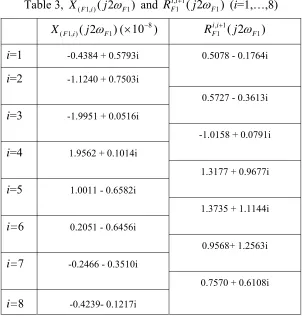
Table 3, X_(F1,i)(j2ω_F1) and R_Fi,i₁+1(j2ω_F1) (i=1,…,8)

) 2 ( ₁

) , 1

(F i j F

X ω (×10−8) R_Fi,₁i+1(j2ω_F1) i=1 -0.4384 + 0.5793i 0.5078 - 0.1764i

i=2 -1.1240 + 0.7503i

0.5727 - 0.3613i

i=3 -1.9951 + 0.0516i

-1.0158 + 0.0791i

i=4 1.9562 + 0.1014i

1.3177 + 0.9677i

i=5 1.0011 - 0.6582i

1.3735 + 1.1144i

i=6 0.2051 - 0.6456i

0.9568+ 1.2563i

i=7 -0.2466 - 0.3510i

i=8 -0.4239- 0.1217i

0.7570 + 0.6108i

In this case study, the 4th spring are nonlinear, that is L = 4. The two sinusoidal forces used

are u₁(t)=sin(2π×20t) and u₂(t)=sin(2π×40t) respectively, and were imposed on the

6th mass of this system, that is J = 6. The responses of the system were obtained using a

fourth-order Runge–Kutta method to integrate equation (31). The second super-harmonics

were used to calculate , 1( 2 ₁), which were extracted from the FFT spectra of the

1 F

i i F j

responses of the system subjected to . The results of the second super-harmonics are given in Table 3 together with the calculated values of (i=1,…,7). Table 4

gives the first harmonics of the FFT spectra of the responses of the system subjected to , together with the values of (i=1,…,7). The moduli of and

(i=1,…,7) are given in Table 5.

) (

1 t

u

) 2 ( ₁

1 ,

1 F

i i F j

R + ω

) (

2 t

u R_Fi,i₂+1(jω_F2) R_Fi,₁i+1(j2ω_F1)

) ( ₂

1 ,

2 F

i i F j

R + ω

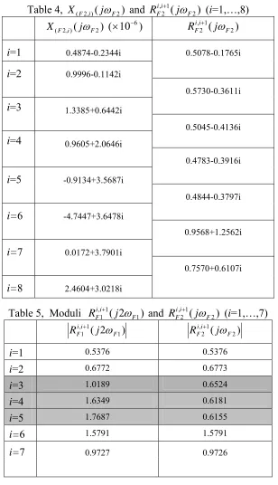
Table 4, X₍F_2,i₎(jωF₂) and ( 2) (i=1,…,8) 1

,

2 F

i i F j

R + ω

) ( ₂

) , 2

(F i j F

X ω (×10−6) R_Fi,i₂+1(jω_F2)

i=1 0.4874-0.2344i 0.5078-0.1765i

i=2 0.9996-0.1142i

0.5730-0.3611i

i=3 _{1.3385+0.6442i}

0.5045-0.4136i

i=4 _{0.9605+2.0646i}

0.4783-0.3916i

i=5 -0.9134+3.5687i

0.4844-0.3797i

i=6 -4.7447+3.6478i

0.9568+1.2562i

i=7 0.0172+3.7901i

i=8 2.4604+3.0218i

0.7570+0.6107i

Table 5, Moduli R_Fi,i₁+1(j2ω_F1) and R_Fi,i₂+1(jω_F2) (i=1,…,7)

) 2 ( 1 1

,

1 F

i i F j

R + ω i,i₂1( _F2)

F j

R + ω

i=1 0.5376 0.5376 i=2 0.6772 0.6773 i=3 1.0189 0.6524

i=4 1.6349 0.6181 i=5 1.7687 0.6155

i=6 1.5791 1.5791

The results given in Table 6 clearly show that ≠ at i = 3,4,5.

According to the detection method in Section 4, it can be known that the component on the right side of the 3

) 2 ( ₁

1 ,

1 F

i i F j

R + ω R_Fi,i₂+1(jω_F2)

rd _{mass is the nonlinear one, that is, the 4}th _{spring component.}

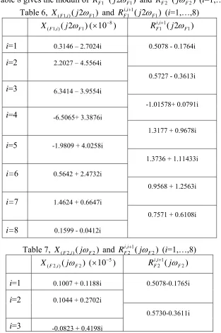
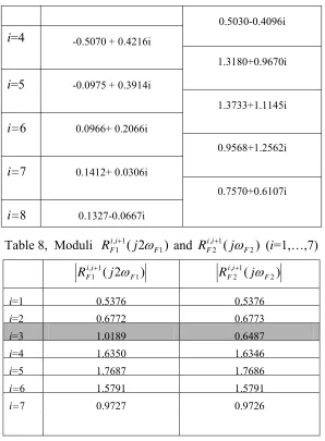
Case Study 2 (L = J):

In this case study, the 4th spring are nonlinear, that is L=4. The sinusoidal forces used in

this case are the same as the ones used in Case 1, but were imposed on the 4th mass of this system, that is J=4, so L=J. The results of X_(F1,i)(j2ω_F1) and (i=1,…,8) are

given in Table 6, and the results of

) 2 ( ₁

1 ,

1 F

i i F j

R + ω

) ( ₂

) , 2

(F i j F

X ω and (i=1,…,8) are given

in Table 7. Table 8 gives the moduli of and (i=1,…,7).

) ( ₂

1 ,

2 F

i i F j

R + ω

) 2 ( ₁

1 ,

1 F

i i F j

R + ω R_Fi,i₂+1(jω_F2)

Table 6, X₍F_1,i₎(j2ωF₁) and ( 2 1) (i=1,…,8) 1

,

1 F

i i F j

R + ω

) 2 ( ₁

) , 1

(F i j F

X ω (×10−8) R_Fi,₁i+1(j2ω_F1)

i=1 0.3146 – 2.7024i 0.5078 - 0.1764i

i=2 2.2027 – 4.5564i

0.5727 - 0.3613i

i=3 _{6.3414 – 3.9554i}

-1.01578+ 0.0791i

i=4 _{-6.5065+ 3.3876i}

1.3177 + 0.9678i

i=5 -1.9809 + 4.0258i

1.3736 + 1.11433i

i=6 0.5642 + 2.4732i

0.9568 + 1.2563i

i=7 1.4624 + 0.6647i

i=8 0.1599 - 0.0412i

0.7571 + 0.6108i

Table 7, X₍F_2,i₎(jωF₂) and ( 2) (i=1,…,8) 1

,

2 F

i i F j

R + ω

) ( ₂

) , 2

(F i j F

X ω (×10−5) R_Fi,i₂+1(jω_F2)

i=1 0.1007 + 0.1188i 0.5078-0.1765i

i=2 0.1044 + 0.2702i

i=3 _{-0.0823 + 0.4198i}

0.5030-0.4096i

i=4 _{-0.5070 + 0.4216i}

1.3180+0.9670i

i=5 -0.0975 + 0.3914i

1.3733+1.1145i

i=6 0.0966+ 0.2066i

0.9568+1.2562i

i=7 0.1412+ 0.0306i

i=8 0.1327-0.0667i

0.7570+0.6107i

Table 8, Moduli R_Fi,i₁+1(j2ω_F1) and R_Fi,i₂+1(jω_F2) (i=1,…,7)

) 2 ( ₁

1 ,

1 F

i i F j

R + ω ,₂1( F₂)

i i F j

R + ω

i=1 0.5376 0.5376 i=2 0.6772 0.6773 i=3 1.0189 0.6487 i=4 1.6350 1.6346 i=5 1.7687 1.7686 i=6 1.5791 1.5791

i=7 0.9727 0.9726

The results given in Table 8 clearly show that ≠ only at i = 3.

According to the detection method in Section 4, it can be known that the component on the right side of the 3

) 2 ( ₁

1 ,

1 F

i i F j

R + ω ,21( F2)

i i F j

R + ω

rd _{mass is the nonlinear one, that is, the 4}th _{spring component.}

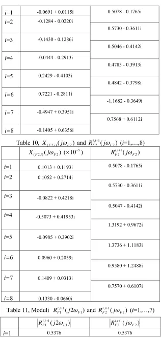
Case Study 3 (L>J):

In this case study, the 7th _{spring are nonlinear, that is}

L=7. The sinusoidal forces used in

this case are the same as the ones used above cases, but were imposed at the 4th _{mass of this}

system, that is J=4, so L>J. The results of X_(F1,i)(j2ω_F1), R_Fi,i₁+1(j2ω_F1), X₍F_2,i₎(jωF₂) and (i=1,…,8) are given in Table 9 and Table 10 respectively. Table 11

gives the moduli of and (i=1,…,7).

) ( ₂

1 ,

2 F

i i F j

R + ω

) 2 ( ₁

1 ,

1 F

i i F j

R + ω ,21( F2)

i i F j

R + ω

Table 9, X_(F1,i)(j2ω_F1) and R_Fi,i₁+1(j2ω_F1) (i=1,…,8)

) 2 ( ₁

) , 1

(F i j F

i=1 -0.0691 + 0.0115i 0.5078 - 0.1765i i=2 -0.1284 - 0.0220i

0.5730 - 0.3611i

i=3 -0.1430 - 0.1286i

0.5046 - 0.4142i

i=4 -0.0444 - 0.2913i

0.4783 - 0.3913i

i=5 0.2429 - 0.4103i

0.4842 - 0.3798i

i=6 0.7221 - 0.2811i

-1.1682 - 0.3649i

i=7 -0.4947 + 0.3951i

i=8 -0.1405 + 0.6356i

0.7568 + 0.6112i

Table 10, X_(F2,i)(jω_F2) and R_Fi,i₂+1(jω_F2) (i=1,…,8)

) ( ₂

) , 2

(F i j F

X ω (×10−5) R_Fi,i₂+1(jω_F2)

i=1 0.1013 + 0.1193i 0.5078 - 0.1765i

i=2 0.1052 + 0.2714i

0.5730 - 0.3611i

i=3 _{-0.0822 + 0.4218i}

0.5047 - 0.4142i

i=4 _{-0.5073 + 0.41953i}

1.3192 + 0.9672i

i=5 -0.0985 + 0.3902i

1.3736 + 1.1183i

i=6 0.0960 + 0.2059i

0.9580 + 1.2488i

i=7 0.1409 + 0.0313i

i=8 0.1330 - 0.0660i

0.7570 + 0.6107i

Table 11, Moduli R_Fi,₁i+1(j2ω_F1) and R_Fi,i₂+1(jω_F2) (i=1,…,7)

) 2 ( ₁

1 ,

1 F

i i F j

R + ω i,i₂1( _F2)

F j

R + ω

i=2 0.6772 0.6773

i=3 0.6528 0.6529

i=4 0.6179 1.6357 i=5 0.6154 1.7712 i=6 1.2238 1.5740

i=7 0.9727 0.9726

The results given in Table 11 clearly show that at i = 4, 5, 6.

According to the detection method in Section 4, it can be known that the component on the right side of the 6

) 2 ( ₁

1 ,

1 F

i i F j

R + ω ≠ i,i₂1( _F2) F j

R + ω

th _{mass is the nonlinear one, that is, the 7}th _{spring component.}

6 Conclusions and Remarks

Based on the properties of NOFRFs, a novel method is developed to detect the position of the nonlinear component in a periodic structure. The detection procedure requires exciting the nonlinear system under study twice using two sinusoidal inputs separately. The frequencies of the two inputs are different; one frequency is twice as high as the other one. Three numerical studies have been used to demonstrate the effectiveness of this method. The distinct advantage of this method is that it only needs the test data under two sinusoidal input forces, which can be readily carried out in practices. Since the positions of the nonlinear components in periodic structures often correspond to the locations of faults, the nonlinear component position detection method is of practical significance in the fault diagnosis for mechanical and structural systems. It is worthy to note here that in real periodic structures there are always minor non-linearities between each component and, such structures therefore should be better to model as weakly nonlinear chains which have been by Chakraborty and Mallik [12]. For such structures, the problem is then changed to detect the components with strong nonlinear property in the weakly nonlinear chains. It is a more complicated problem we are planning to investigate in future studies.

Acknowledgements

References

1. D. Duhame, B.R. Maceb, M.J. Brennan, Finite element analysis of the vibrations of waveguides and periodic structures, Journal of Sound and Vibration294 (2006) 205-220

2. A. Luongo, F. Romeo, Real wave vectors for dynamic analysis of periodic structures,

Journal of Sound and Vibration279 (2005) 309–325

3. F.Romeo, A.Luongo, Vibration reduction in piecewise bi-coupled periodic structures,

Journal of Sound and Vibration268 (2003) 601–615

4. J. Wei, M. Petyt, A method of analyzing finite periodic structures, Part 1: Theory and examples, Journal of Sound and Vibration, 202 (1997) 555-569

5. S. Mukherjee, S. Parthan, Normal modes and acoustic response of finite one- and

two-dimensional multi-bay periodic panels. Journal of Sound and Vibration, 197

(1996) 527-545

6. J. Yuan, S. M. Dickinson, On the determination of phase constants for the study of the free vibration of periodic structures, Journal of Sound and Vibration, 179 (1995)

369-383

7. S. D. Fassois, J.S. Sakellariou, Stochastic output error vibration-based damage detection and assessment in structures under earthquake excitation, Journal of Sound and Vibration 297(2006), 1048-1067

8. D.J. Mead, Wave propagation in continuous periodic structures: research

contributions from Southampton, 1964-1995, Journal of Sound Vibration. 190 (1996) 495-524.

9. C-C Chi, R. M. Rosenberg, On damped Non-linear Dynamic systems with many degrees of freedom, International Journal of Non-Linear Mechanics. 20 (1985) 371-384

10.A. F. Vakakis, M. E. King and A. J. Pearlstein, Forced Localization in a periodic chain of non-linear oscillators, International Journal of Non-Linear Mechanics.

29(1994) 429-447

11.T. J. Royston, R. Singh, Periodic response of mechanical systems with local non-linearities using an enhanced Galerkin technique, Journal of Sound and Vibration,

194 (1996) 243-263

13.Amol Marathe, Anindya Chatterjee, Wave attenuation in nonlinear periodic structures using harmonic balance and multiple scales, Journal of Sound and Vibration289 (2006) 871–888

14.S.A. Neild, P.D. Mcfadden and M.S Williams, A discrete model of vibrating beam using time-stepping approach. Journal of Sound and Vibration 239(2001), 99-121

15.H. Zhu, M. Wu, The Characteristic receptance method for damage detection in large Mono-coupled Periodic structures, Journal of Sound and Vibration 251(2002), 241-259

16.S. D. Fassois, J.S. Sakellariou, Time-series methods for fault detection and

identification in vibrating structures, Philosophical Transactions of the Royal Society A: Mathematical, Physical and Engineering Sciences, 365 (2007) 411 – 448

17.K. Worden, G. Manson, G.R. Tomlinson, A harmonic probing algorithm for the multi-input Volterra series. Journal of Sound and Vibration201(1997) 67-84 18.Z. Q. Lang, S. A. Billings, Output frequency characteristics of nonlinear system,

International Journal of Control 64 (1996) 1049-1067.

19.S.A. Billings, K.M. Tsang, Spectral analysis for nonlinear system, part I: parametric non-linear spectral analysis. Mechanical Systems and Signal Processing, 3 (1989) 319-339

20.S.A. Billings, J.C. Peyton Jones, Mapping nonlinear integro-differential equations into the frequency domain, International Journal of Control52 (1990) 863-879. 21.J.C. Peyton Jones, S.A. Billings, A recursive algorithm for the computing the

frequency response of a class of nonlinear difference equation models. International Journal of Control50 (1989) 1925-1940.

22.Z. Q. Lang, S. A. Billings, Energy transfer properties of nonlinear systems in the frequency domain, International Journal of Control78 (2005) 354-362.

23.ZK Peng, ZQ Lang, SA Billings, Nonlinear Output Frequency Response Functions of MDOF Systems with Multiple Nonlinear Components, International Journal of Non-linear Mechanics (2007), Doi:10.1016/j.ijnonlinmec.2007.04.001

24.Z.Q Lang, S. A. Billings, Output frequencies of nonlinear systems, International Journal of Control, 67 (1997)713~730.