This is a repository copy of Non-linear protocols for optimal distributed consensus in networks of dynamic agents..
White Rose Research Online URL for this paper: http://eprints.whiterose.ac.uk/89771/
Version: Accepted Version
Article:
Bauso, D., Giarré, L. and Pesenti, R. (2006) Non-linear protocols for optimal distributed consensus in networks of dynamic agents. Systems & Control Letters, 55 (11). 918 - 928. ISSN 0167-6911
https://doi.org/10.1016/j.sysconle.2006.06.005
[email protected] https://eprints.whiterose.ac.uk/ Reuse
Unless indicated otherwise, fulltext items are protected by copyright with all rights reserved. The copyright exception in section 29 of the Copyright, Designs and Patents Act 1988 allows the making of a single copy solely for the purpose of non-commercial research or private study within the limits of fair dealing. The publisher or other rights-holder may allow further reproduction and re-use of this version - refer to the White Rose Research Online record for this item. Where records identify the publisher as the copyright holder, users can verify any specific terms of use on the publisher’s website.
Takedown
If you consider content in White Rose Research Online to be in breach of UK law, please notify us by
Nonlinear protocols for optimal distributed
consensus in networks of dynamic agents
D. Bauso,
bL. Giarr´e
a,1and R. Pesenti
ba Dipartimento di Ingegneria dell’Automazione e dei Sistemi
Universit`a di Palermo, Viale Delle Scienze, 90128 Palermo, Italy.
b Dipartimento di Ingegneria Informatica
Universit`a di Palermo, Viale Delle Scienze, 90128 Palermo, Italy.
{dario.bauso,pesenti}@unipa.it
Abstract
We consider stationary consensus protocols for networks of dynamic agents with fixed topologies. At each time instant, each agent knows only its and its neighbors’ state, but must reach consensus on a group decision value that is function of all the agents’ initial state. We show that the agents can reach consensus if the value of such a function is time-invariant when computed over the agents’ state trajecto-ries. We use this basic result to introduce a non-linear protocol design rule allowing consensus on a quite general set of values. Such a set includes, e.g., any general-ized mean of order pof the agents’ initial states. As a second contribution we show that our protocol design is the solution of individual optimizations performed by the agents. This notion suggests a game theoretic interpretation of consensus prob-lems as mechanism design probprob-lems. Under this perspective a supervisor entails the agents to reach a consensus by imposing individual objectives. We prove that such objectives can be chosen so that rational agents have a unique optimal protocol, and asymptotically reach consensus on a desired group decision value. We use a Lyapunov approach to prove that the asymptotical consensus can be reached when the communication links between nearby agents define a time-invariant undirected network. Finally we perform a simulation study concerning the vertical alignment maneuver of a team of unmanned air vehicles.
Key words: Consensus Protocols, Decentralized Control, Optimal Control, Networks
1 Corresponding author L. Giarr´e, Research supported by PRIN “Robustness optimization
1 Introduction
Distributed consensus protocols are distributed control policies based on local information that allow the coordination of multi-agent systems. Agents implement a consensus protocol to reach consensus, that is to (make their states) converge to a same value, called consensus-value, or group decision value [1,2].
Coordination of agents/vehicles is an important task in several applications including au-tonomous formation flight [3,4], cooperative search of unmanned air-vehicles (UAVs) [5], swarms of autonomous vehicles or robots [6–8], multi-retailer inventory control [9–11] and congestion/flow control in communication networks [12].
Particularly interesting is the progress in the design and analysis of consensus protocols ob-tained merging notions and tools from the Graph Theory and Control Theory [13]. Actually, a central point in consensus problems is the connection between the graph topology, possi-bly switching, and delays or distortions in communication links [14]. Switching topology and directional communications are studied in [1,15–19], while cooperation based on the notion of coordination variable and coordination function in [20,21]. There, coordination variable is referred to as the minimal amount of information needed to effect a specific coordination ob-jective, whereas a coordination function parameterizes the effect of the coordination variable on the myopic objectives of each agent.
In this paper, n dynamic agents reach consensus on a group decision value by implement-ing optimal, distributed and stationary control policies based on neighbors’ state feedback. Here, neighborhood relations are defined by the existence of communication links between nearby agents. We assume that the set of communication links are bidirectional and define a time-invariant connected communication network. In this context, we argue that agents asymptotically reach consensus on the desired group decision value by studying equilibrium properties and stability of the group decision value via Lyapunov theory. Similarly to [1,3,13], our agents follow a first-order dynamics. We restrict the group decision value to be a permu-tation invariant function of the agents’ initial states. Permutation invariance means that the value of the function is independent of the agents indexes.
intelligence has on one hand a non insdifferent cost due to the necessity of equipping each agent with computational and processing units, but, on the other hand, reduces the monitor-ing costs. We show that, if the supervisor imposes convex penalty functions, rational agents have a unique optimal protocol. We prove this result through the Pontryagin Minimum Prin-ciple (see, e.g., [26]). From a slightly different point of view, the solution of a mechanism design problem allows to determine whether a set of agents with given individual objective functions will implement the considered protocol.
The present paper states consensus protocol definition and mechanism design as two separate problems for the sake of clarity. However, it must be noted that these two problems may be seen as two faces of the same coin. The consensus protocol definition problem answers to the question of determining the policies that the agents must implement to reach a given consensus. The mechanism design problem answers to the question of which policy is imple-mented, and hence which consensus value is reached, by selfish agents with given individual objectives.
Unfortunately, solving the mechanism design problem is a difficult task, unless the problem is an affine quadratic game [23]. Our idea is then to translate it into a sequence of more tractable receding horizon problems. At each discrete time tk, the receding horizon control scheme optimizes over an infinite planning horizon T → ∞, and executes the controls over a one-step action horizon δ = tk+1−tk [27,28]. The neighbors’ state whose evolution is un-predictable, are kept constant over the planning horizon (naive assumption) [29,30]. At time
tk+1 each agent re-optimizes its controls based on the new information on neighbors’ state which has become available. To find an approximate solution to Problem 2 we then take the limit for δ→0 of the given receding horizon solution.
The paper is organized as follows. In Section 2, we formulate the consensus problem (Prob-lem 1) and the mechanism design prob(Prob-lem (Prob(Prob-lem 2). Section 3 and 4 concern the solution to the consensus problem. In particular, in Section 3, we study the time invariancy property of the state trajectory. In Section 4, we provide sufficient conditions for the asymptotical stability of the group decision value via Lyapunov theory. Section 5 addresses the mechanism design problem, whose solution is derived starting from the results on the consensus prob-lem. More specifically, we exploit the Pontryagin Minimum Principle to derive necessary and sufficient optimality conditions. Then, we merge the results on time invariancy, stability, and optimality to design a mechanism for the distributed optimal consensus. In Section 6, we simulate the vertical alignment maneuver of a team of UAVs. Finally, in Section 7, we draw some conclusions.
2 Consensus and Mechanism Design Problems
Each edge (i, j) in the edgeset E means that there is communication from j to i. As (j, i) is also in the edgeset E the communication is bidirectional, namely, if agent i can receive information from agentj then also agentj can receive information from agenti. Also,Gnot complete means that each agent i exchanges information only with its neighbors.
Each agentihas a (simplified)first-order dynamics controlled by adistributed andstationary control policy
˙
xi =ui(xi, x(i)) ∀i∈Γ, (1)
where xi is the state of agent i and x(i) is the state vector of the agents in Ni with generic
component j defined as follows,x(i)j =
xj if j ∈Ni,
0 otherwise,
and such that (1) has unique solutions. The policy is distributed since, for each agent i, it depends only on the local information available to it, which isxiandx(i). No other information on the current or past system state is available to agent i. (We discuss the limitation of this assumption at the beginning of Section 3). The policy is stationary since it does not depend explicitly on time t. In other words, the policy is a time-invariant and memoryless function of the state. Define the system state vector x(t) = {xi(t), i ∈ Γ}, then the system initial state x(0) is the collection of the agents’ initial states. Define u(x) = {ui(xi, x(i)) : i ∈ Γ} as a distributed stationary protocol or simply a protocol. Let ˆχ : IRn → IR be a generic continuous and differentiable function ofnvariablesx1, . . . , xnwhich is permutation invariant, i.e., ˆχ(x1, x2, . . . , xn) = ˆχ(xσ(1), xσ(2), . . . , xσ(n)) for any one to one (permutation) mapping
σ(.) from the set Γ to the set Γ. Henceforth ˆχ is also called agreement function. Putting together slightly different definitions in [1,2,22], we say that a protocolu(.) makes the agents asymptotically reach consensus on a group decision value χˆ(x(0)) function of their initial states if kxi −χˆ(x(0))k −→ 0 as t −→ ∞. When this happens we also say that the system converges to ˆχ(x(0))1. Here and in the following, 1 stands for the vector (1,1, . . . ,1)T. Notwithstanding each agent i has only a local information (xi, x(i)) about the system state
x, we are interested in making the agents reach consensus on group decision values that are functions of the whole system initial statex(0). In particular, we are interested in agreement functions verifying
min
i∈Γ{yi} ≤χˆ(y)≤maxi∈Γ {yi}, for all y∈IR n
. (2)
The above condition means that the group decision value must be confined between the minimum and the maximum values of the agents’ initial states.
Finally, we define an individual objective for an agent i, i.e.,
Ji(xi, x(i), ui) = lim T−→∞
T
Z
0
F(xi, x(i)) +ρu2i
where ρ > 0 and F : IR×IRn → IR is a nonnegative penalty function that measures the deviation of xi from neighbors’ states. We say that a protocol isoptimal if each ui optimizes the corresponding individual objective.
In the above context, we face the following problem.
Problem 1 (Consensus Problem) Consider a network G = (Γ, E) of dynamic agents with
first-order dynamics. For any agreement function χˆ satisfying condition (2), determine a (distributed stationary) protocol, whose components have the feedback form (1), that makes the agents asymptotically reach consensus on χˆ(x(0)) for any initial state x(0).
In the following, a protocol that solves the consensus problem is also referred to as aconsensus protocol. In addition a consensus protocol is said optimal, if its components are the optimal controls ui(.) corresponding to minimizing (3).
Problem 2 (Mechanism design problem) Consider a networkG= (Γ, E)of dynamic agents
with first-order dynamics. For any agreement function χˆ(.) determine a penalty functionF(.) such that there exists an optimal consensus protocolu(.)with respect toχˆ(x(0))for any initial state x(0).
Notice that a pair (F(.), u(.)) solving Problem 2 must be such that all individual objectives (3) converge to a finite value. Then, it is necessary that the integrand in (3) be null if computed inχ1. We will check later on that this necessary condition is verified by our candidate penalty function F(.).
3 Time Invariancy of χˆ(x(t))
In this section and in the following one we focus on Problem 1. Initially, we show that if a protocol, which solves a consensus problem, is distributed and stationary then the system state trajectory enjoys the property that ˆχ(x(t)) is time-invariant. Then, we find a family of non trivial protocols that guarantee such a property. We prove that some of such protocols are consensus protocols with respect to ˆχ(x(0)) in the next section.
Lemma 1 (Time invariancy) Consider a network G= (Γ, E) of dynamic agents with
first-order dynamics. For an agreement function χˆ assume there exists a distributed stationary protocol u(.), whose components have the feedback form (1), that makes the agents asymp-totically reach consensus on χˆ(x(0)) for any initial state x(0). Then the value of χˆ(x(t)) is time-invariant, i.e., χˆ(x(t)) = ˆχ(x(0)) for all t >0.
Proof. The key idea is that the protocols used are time-invariant (so the system of differential equations (1) is autonomous) and such that the system has unique solutions. Since the system is autonomous and by assumption x(t)→χˆ(x(0))1as t→ ∞, thenys(t) = x(t+s) is also a solution (with ys(0) = x(s)) and we also have ys(t) →χˆ(ys(0))1 as t → ∞ for any s. Since
From continuity of function ˆχ and supposing that the state trajectory reaches the point ˆ
χ(x(0))1, the time invariancy property stated in Lemma 1 implies also that ˆχ(x(0)) = ˆ
χ( ˆχ(x(0))1). Note that the last condition satisfies (2). Actually, (2) imposes that function ˆ
χ(.) must be chosen such that any point λ1, for all λ ∈IR, is a fixed point, i.e., ˆχ(λ1) = λ, as it can be trivially derived assuming y=λ1.
With this consideration in mind, let us impose the time invariancy of ˆχ(x(t)) to derive a necessary property for the consensus protocol. As it holds ˆχ(x(t)) =const then
dχˆ(x(t))
dt =∇xχˆ(x)·x˙ =
X
i∈Γ
∂χˆ(x)
∂xi
˙
xi =
X
i∈Γ
∂χˆ(x)
∂xi
ui = 0. (4)
The trivial protocol constantly equal to 0 leaves any value ˆχ(x(t)) time-invariant, for any possible ˆχ(.), but obviously does not make the system converge. Consequently, it is no longer considered hereafter.
Some other solutions of equation (4) can be obtained easily when ˆχ(x) presents a particular structure. A first possibility is when the following condition holds
∂χˆ(x)
∂xi
ui = 0 ∀i∈Γ. (5)
For example, ˆχ(x) = min{xi} and ui = h(xi,minj∈Ni{xj}) satisfy the above condition, for
any h(x, y) : IR2 →IR such that h(x, y) = 0 when x =y. Actually, ∂ˆ∂xχ(x)
i 6= 0 only for i such
that xi = minj∈Γ{xj}, then, by definition of functionh(.), it holds ui(xi) = 0 and hence (5). Note that though ˆχ(x) = min{xi}is not differentiable, at points where the partial derivative
∂χ(x)ˆ
∂xi is not defined the protocol ui = 0. The system converges to ˆχ(x(0)) if we impose
the additional condition h(x, y) < 0 when x > y. Trivially, analogous argument applies to ˆ
χ(x) = max{xi}.
We specialize our study considering the following family of agreement function ˆχ(x).
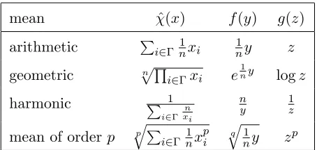
Assumption 1 (Structure ofχˆ(.)) Assume that the generic agreement function χˆ(.)satisfies condition (2) and is such that χˆ(x) = f(P
i∈Γg(xi)), for some f, g : IR →IR with dg(xdxii) 6= 0 for all xi.
A point of interest is that the above family of agreement function is more general than the arithmetic/min/max means already reported in the literature (see, e.g., Tab. 1). In this sense, observe that the structure of the agreement function is general to the extent that any value in the range between the minimum and the maximum values of the agents’ initial states can be chosen as a group decision value. To see this, it is sufficient to consider mean of order p
with p varying between −∞ and ∞.
Theorem 1 (Protocol design rule) For any agreement function χˆ(.)as in Assumption 1, the
non trivial protocol
ui(xi, x(i)) =
1 dg(xi)
dxi X
j∈Ni
mean χˆ(x) f(y) g(z)
arithmetic P
i∈Γ 1nxi 1
ny z
geometric pQn
i∈Γxi e 1
ny logz
harmonic P 1
i∈Γ
n xi n y 1 z
mean of order p qp P
i∈Γ 1nx p i
q q
1 ny z
[image:8.612.183.410.56.164.2]p
Table 1
Means under consideration and their representations in terms of f and g
lets the value χˆ(x(t)) be time-invariant if φ : IR2 → IR is an antisymmetric function, i.e.,
φ(xj, xi) =−φ(xi, xj).
Proof. A sufficient condition for ˆχ(x(t)) being time-invariant is that its argumentP
i∈Γg(xi(t)) is time-invariant, too. The latter condition means
X
i∈Γ
dg(xi(t))
dt =
X
i∈Γ
dg(xi)
dxi
˙
xi =
X
i∈Γ
dg(xi)
dxi
ui = 0.
It is immediate to verify that protocol (6) satisfies conditionP
i∈Γdg(xdxii)ui = 0. Actually, since φ is antisymmetric and the links are bidirectional then we haveP
i∈Γ
P
j∈Niφ(xj, xi) = 0. 2
Consider the linear function φ(xj, xi) = α(xj −xi) and the different means introduced in Tab. 1. The arithmetic mean is time-invariant under protocol u(xi, x(i)) =αPj∈Ni(xj −xi);
the geometric mean under protocolu(xi, x(i)) = αxiPj∈Ni(xj−xi); the harmonic mean under
protocol u(xi, x(i)) = −αx2i
P
j∈Ni(xj−xi); the mean of order p under protocol u(xi, x
(i)) =
αx1i−p
p
P
j∈Ni(xj −xi).
Obviously, due to the time invariancy of ˆχ(x(t)) if the system converges, it will converge to ˆ
χ(x(0))1, but it does not necessarily converge. As it turns out at the end of the next section, for the cases in the example, the system converges to ˆχ(x(0))1only ifα >0 (for the harmonic mean only if α <0). In addition, we must also assume that xi(0)>0 for all i∈Γ, when we deal with means different from the arithmetic one.
4 Sufficient conditions for convergence
In the previous section, we find a family of protocols as in (6) that guarantees the time invariancy of ˆχ(x(t)). In this section, we determine sufficient conditions on the structure of functions g(.) and φ(.) such that a protocol of type (6) makes the system converge to
ˆ
χ(x(0))1 for any agreement function ˆχ(.) and initial statex(0). In particular, we prove that the system converges when the function g(.) is strictly increasing and the function φ(.) is defined as follows:
whereα >0, function ˆφ: IR→IR is continuous, locally Lipschitz, odd and strictly increasing, and function ϑ: IR→IR is differentiable with dϑ(xi)
dxi locally Lipschitz and strictly positive.
Putting together (6) and (7) the resulting protocol is
ui(xi, x(i)) =α
1 dg dxi
X
j∈Ni
ˆ
φ(ϑ(xj)−ϑ(xi)), for all i∈Γ. (8)
Initially, we study the stability of the system under protocol (8).
Lemma 2 Consider a network G= (Γ, E) of dynamic agents with first-order dynamics and
implement a distributed and stationary protocol u(.) whose components have the feedback form (8). Then, all equilibria are of the form λ1 and if a trajectoryx(t) converges asymptot-ically to the equilibrium λ01 then λ0 = ˆχ(x(0)), for any initial state x(0).
Proof. First, we show that any equilibrium pointx∗ must have all its component equal, i.e.,
x∗ =λ1 where λ is a constant value. Then we prove thatλ is equal to ˆχ(x(0)).
Sufficiency. Assume,xi =λ, for alli∈Γ, thenuiφˆ(ϑ(λ)−ϑ(λ)) = 0 since ˆφ(.) is continuous and odd. Thus, the point x∗ =λ1 is an equilibrium point.
Necessity. Assume that there exists an equilibrium point x∗ 6= λ1. We prove that such an
assumption implies the existence of at least one agent i with ui < 0, and this last result contradicts the definition of equilibrium for x∗. Define I ={i∈ Γ :x∗
i ≥ x∗j, ∀j ∈ Γ} as the set of agents with maximum state value. Trivially,Iis included but not equal to Γ, asx∗ 6=λ1.
Then, i and j with (i, j) ∈ E such that x∗
i 6= x∗j exist, since the network G is connected. In particular, we can always choose i ∈ I such that there exists j ∈ Ni with x∗j < x∗i. Now observe that, since ˆφ(.) is an odd and strictly increasing and ϑ(.) is strictly increasing, then
P
j∈Niφˆ(ϑ(x
∗
j)−ϑ(x∗i))<0. Actually, all the terms of the sum are non positive and at least one is strictly negative. Since it also holds that α dg1
dxi
6
= 0, the contradiction is proved.
Convergence. The above arguments show that ˆχ(x(0))1is an equilibrium point. Now, we prove by contradiction that λ = ˆχ(x(0)). Indeed, if λ = ˆ6 χ(x(0)), then ˆχ(x) under protocol (8) is no longer time invariant. Let us assume that the system actually converges to a different equilibrium point x∗ = λ1 6= ˆχ(x(0))1. As ˆχ(.) enjoys the fixed point property, we have
ˆ
χ(x∗) =λ 6= ˆχ(x(0)).
2
We are now ready to prove that the agents asymptotically reach consensus on ˆχ(x(0))1when function g(.) is strictly increasing, i.e., dg(y)dy >0 for all y∈IR.
Theorem 2 Consider a network G = (Γ, E) of dynamic agents with first-order dynamics
and implement a distributed and stationary protocol whose components have the feedback form (8). If function g(.) is strictly increasing, the agents asymptotically reach consensus on
ˆ
χ(x(0))1 for any initial state x(0).
Proof. We follow a line of reasoning similar to the one in [1]. First, observe that consensus reaching corresponds to asymptotic stability of a new variable η = {ηi, i ∈ Γ}, where ηi =
strictly increasing asg(.), andη= 0 corresponds tox= ˆχ(x(0))1. We prove the asymptotical stability (in the quotient space IRn/span{1}) of the equilibrium point η= 0 by introducing a candidate Lyapunov function V(η) = 12P
i∈Γηi2. Trivially, V(η) = 0 if and only if η = 0;
V(η)>0 for all η6= 0. It remains to prove that ˙V(η)<0 for all η6= 0.
˙
V(η) =X
i∈Γ
ηiη˙i =
X
i∈Γ
ηi
dg(xi)
dxi
˙
xi = (9a)
=X
i∈Γ
ηi
dg(xi)
dxi
ui =
X
i∈Γ
ηi
dg(xi)
dxi
α dg1
dxi X
j∈Ni
ˆ
φ(ϑ(xj)−ϑ(xi)) = (9b)
=αX
i∈Γ
ηi
X
j∈Ni
ˆ
φ(ϑ(xj)−ϑ(xi)) = (9c)
=−α X
(i,j)∈E
(g(xj)−g(xi)) ˆφ(ϑ(xj)−ϑ(xi)) (9d)
In (9) we simply expressηi and ˙ηi in terms of the state variables and their derivatives.2 To get (9d) from (9c), we reorder the terms and exploit the fact thatj ∈Ni if and only ifi∈Nj for each i, j ∈Γ. From (9d) we have ˙V(η)≤0 for all η and, in particular, ˙V(η) = 0 only for
η = 0. Actually, as α > 0 and g(.), ˆφ(.), and ϑ(.) are strictly increasing, we have that, for any (i, j)∈E, xj > xi impliesg(xj)−g(xi)>0,ϑ(xj)−ϑ(xi)>0 and ˆφ(ϑ(xj)−ϑ(xi))>0. Hence, we obtain α(g(xj)−g(xi)) ˆφ(ϑ(xj)−ϑ(xi)) > 0 if xj > xi. Trivially, a symmetrical argument holds if xj < xi. 2
It is possible to partially relax the assumptions of Theorem 2 concerning the monotonicity of function g(.). The reason is evident from the following theorem establishing that all agents’ state trajectories are bounded.
Theorem 3 Assume all the conditions in Theorem 2 hold. Then, condition (7) implies that
for all i∈Γ and t ≥0
min
j∈Γ{xj(0)} ≤xi(t)≤maxj∈Γ{xj(0)}. (10)
Proof. Letα= minj∈Γ{xj(0)}andβ = maxj∈Γ{xj(0)}. The aim is to prove that all solutions stay inside the hypercube [α, β]n. This can be shown by noticing that, for each generic agenti, the state xi(t) is a continuous. Observe, that on the faces of the polyhedron [α, β]n the corresponding vector field does not point outwards. This translates into ui(α, x(i)) ≥0 (and
ui(β, x(i))≤0) which follows immediately from the definition of ui 2
2 Let K=g( ˆχ(x(0))), the dynamics of η can be equivalently expressed as
˙
ηi =α
X
j∈Ni
ˆ
φϑg−1(ηj +K)
−ϑg−1(ηi+K)
Trivially, condition (10) holds even if g(y) is strictly increasing only in the subset of IR defined by minj∈Γ{xj(0)} ≤y≤maxj∈Γ{xj(0)}, since the agents’ state trajectory values are bounded within the same set. The boundedness of the agents’ state trajectories allows us to partially relax the assumptions of Theorem 2 concerning the monotonicity of function g(.). Indeed, Theorem 2 still holds if g(.) is strictly increasing in only a subset X ∈ IR provided that xi(t) ∈ X, for all t ≥ 0 and for all i ∈ Γ. Theorem 3 proves that the latter condition is certainly satisfied if X is a connected subset and xi(0) ∈ X for all i ∈ Γ. As a further trivial generalization of Theorem 2 we observe that it holds even ifg(.) is strictly decreasing. However, in this case, α in (7) must be strictly negative instead of positive.
An immediate consequence of the above considerations is the following. Since the means introduced in Tab. 1 have the component g(.) strictly increasing except the harmonic mean, if we consider the linear function φ(xj, xi) = α(xj −xi), the system converges to ˆχ(x(0))1
for α > 0 except for the harmonic mean where we need α < 0. When we deal with means
different from the arithmetic one we also need that xi(0) > 0 for all i ∈ Γ, since g(y) may not even be defined fory ≤0.
The results to communication networks whose topology switches within set of directed graphs that are connected and balanced can be easily extended via a common Lyapunov function approach, see [31].
5 Penalty Functions and Optimal Protocols
In this section, we adopt a mechanism design perspective. We discuss whether we can make the agents asymptotically reach consensus on the group decision value by assigning to each agent an individual objective function to optimize (Problem 2).
Unfortunately, solving Problem 2 is a difficult task. Our idea is then to translate it into a sequence of more tractable problems (Problem 3). At each discrete time tk, the receding horizon control scheme of Problem 3 optimizes over an infinite planning horizon T → ∞, and executes the controls over a one-step action horizonδ =tk+1−tk. The neighbors’ state whose evolution is unpredictable, are kept constant over the planning horizon (Assumption 2) [29,30]. At time tk+1 each agent re-optimizes its controls based on the new information on neighbors’ state which has become available. To find an approximate solution to Problem 2 we then take the limit for δ→0 of the given receding horizon solution.
The receding horizon update times are tk =t0+δk, where k = 0,1, . . .. The cost of agent i depends on his state and others’ state trajectories as well. Let us denote with ˆxi(τ, tk) and ˆ
x(i)(τ, t
k), τ ≥tk respectively the predicted state of agent iand of his neighbors.
Problem 3 (Receding Horizon) For all agents i ∈ Γ and times tk, k = 0,1, . . ., given the initial state xi(tk), and x(i)(tk) find
ˆ
where
Ji(xi(tk), x(i)(tk),uˆi(τ, tk)) = lim T−→∞
T
Z
tk
F(ˆxi(τ, tk),xˆ(i)(τ, tk)) +ρuˆ2i(τ, tk)
dτ (11)
subject to
˙ˆ
xi(τ, tk) = ˆui(τ, tk) (12a)
˙ˆ
xj(τ, tk) = ˆuj(τ, tk) := 0, ∀j ∈Ni, (12b)
ˆ
xi(tk, tk) =xi(tk) (12c)
ˆ
xj(tk, tk) =xj(tk), ∀j ∈Ni. (12d)
In the above problem, equations (12a) and (12b) predict respectively the evolution of the state of agent i and of his neighbors, and conditions (12c) and (12d) represent the initial state at time tk. Note that whereas agent i may predict with a certain approximation the evolution of its state as described by (12a), nothing can he know about the evolution of the states of his neighbors (12b). In this context, agentiat timetk, k = 0,1, . . .assumes that the states of his neighbors are constant over the planning horizon, that is ˆx(i)(τ, t
k) = x(i)(tk),
∀τ > tk (naive assumption).
According to the standard receding horizon scheme, the agents update the receding horizon control policy when a new initial state updatex(i)(t
k+1) is available. As a result, for alli∈Γ, we have the following closed-loop system
˙
xi =uiRH(τ), τ ≥t0,
where the applied receding horizon control law uiRH(τ) satisfies
uiRH(τ) = ˆu
⋆
i(τ, tk), τ ∈[tk, tk+1).
Once we assume (12b) we have ˆx(i) constant in (11) and the receding horizon problem (Prob-lem 3) reduces to one dimension (in fact, n one-dimensional problems). This is evident, if we explicit dependence of F(.) only on the state ˆxi(τ, tk), and simplify the expression of the individual objective function (11) as
Ji = lim T−→∞
T
Z
tk
F(ˆxi(τ, tk)) +ρuˆ2i(τ, tk)
dτ. (13)
Now, to verify that a given control ˆui(τ, tk) is optimal, we use the Pontryagin Minimum Principle. To do this, first, we must construct the Hamiltonian function (for sake of simplicity dependence on τ and tk is dropped)
H(ˆxi,uˆi, pi) = (F(ˆxi) +ρuˆ2i) +piuˆi. (14)
Second, we must impose the Pontryagin necessary conditions.
Optimality condition: ∂H(ˆxi,uˆi, pi)
∂uˆi
= 0 ⇒ pi =−2ρuˆi. (15)
Multiplier condition: p˙i =−
∂H(ˆxi,uˆi, pi)
∂xˆi
. (16)
State equation: x˙ˆi =
∂H(ˆxi,uˆi, pi)
∂pi
⇒ x˙ˆi = ˆui. (17)
Minimality condition: ∂
2H(ˆx
i,uˆi, pi)
∂uˆ2 i
ˆ
xi=ˆx∗i,ˆui=ˆu∗i,pi=p∗i
≥0 ⇒ρ≥0. (18)
Boundary condition: H(ˆx∗i,uˆ∗i, p∗i) = 0. (19)
This last condition requires that the Hamiltonian must be null along any optimal path
{xˆ∗
i(t),∀t≥0} (see, e.g., [26], Section 3.4.3).
We recall that the Pontryagin Minimum Principle provides necessary but not sufficient op-timality conditions [26]. The above conditions become also sufficient to identify a unique optimal solution if also the following condition holds [26].
Uniqueness condition: F(xi) is convex. (20)
The following theorem states sufficient conditions on the structure ofF(xi) that allow us to determine analytically a unique optimal control policy ˆui(.) .
Theorem 4 Consider an agent i with first-order dynamics, at times tk = 0,1, . . ., assign it an objective function as (11) whose penalty function is
F(ˆxi(τ, tk)) =ρ
1 dg dxi
X
j∈Ni
(ϑ(xj(tk))−ϑ(ˆxi(τ, tk)))
2
(21)
where g(.) is increasing,ϑ(.)is concave, and dg1(y)
dy
is convex. Then the following control policy is the unique optimal solution to Problem 3
ˆ
u⋆i(τ, tk) =ui(xi(τ)) = α
1 dg dxi(τ)
X
j∈Ni
Proof. We first show that the problem of minimizing (13) is well posed by proving that, given a penalty function as in (21), there exists at least a control policy for which objec-tive (13) converges. Second we certificate the optimality of control policy (22) via Pontryagin Minimum Principle and, finally, we prove the uniqueness of the optimal solution by showing that F(.) is convex.
To prove that the problem is well posed, let us start by showing that there exists at least one reachable state x∗
i under a stationary control policy function only of local information (xi, x(i)) in which both the penalty (21) and the control itself are null. Now, the penalty (21) is null in a state ˆx∗
i such that
P
j∈Ni(ϑ(xj(tk))−ϑ(x
∗
i)) = 0. From the latter we also have
x∗
i = ϑ−1
P
j∈Niϑ(xj(tk))
|Ni|
which means that x∗
i can be determined on the basis of the local
information (ˆxi(τ, tk), x(i)(tk)) available to agent i. Therefore there trivially exists a control policy that is null in x∗
i and makes the objective function (13) converge.
Now, to certificate the optimality of control policy (22) withα = 1, let us show that it satis-fies conditions (15)-(20) imposed by the Pontryagin Minimum Principle. Our hypothesis on the agent dynamics and on the structure of the agent objective function trivially satisfy (17) and (18). By computing ˙pi from (15) and substituting the obtained value in (16) we have
2ρu˙ˆi =
∂H(ˆxi,uˆi, pi)
∂xˆi
. (23)
In (17), we can write ˙ˆui = ∂∂ˆuxˆiix˙ˆi = ∂ˆ∂ˆuxiiuˆi. Hence condition (23) becomes 2ρ∂∂uxˆˆiiuˆi = ∂H(ˆx∂ˆix,uˆii, pi). Integrating and imposing condition (19) we obtain that a possible solution of (23) must satisfy
ρuˆ2i =F(ˆxi). (24)
It is immediate to verify that ˆui(τ, tk) = dg1
dxiˆ
P
j∈Ni(ϑ(xj(tk))−ϑ(ˆxi(τ, tk))) satisfies the above
condition.
Finally, to prove that control policy (22) is the unique optimal solution, let us show thatF(ˆxi) is convex. To do this, let us write F =F3(F1(ˆxi),F2(ˆxi)) where function F1(ˆxi) =
∂g
∂xi
−1
, functionF2(ˆxi) =Pj∈Ni(ϑ(xj(tk))−ϑ(ˆxi)) andF3 = (F1(ˆxi)· F2(ˆxi))
2. WithF
3(.) being non decreasing in each argument, function F3(.) is convex if both functions F1(.) and F2(.) are also convex [32]. Function F1(.) is convex as
dg
dˆxi
−1
is convex by hypothesis. Analogously,
F2(.) is convex asϑ(.) is concave. 2
The above theorem holds trivially for α=−1 if dxdg
i <0 for all xi(0).
Note that the optimal control policy (22) is a feedback policy with respect to the only state ˆ
xi whereas is an open-loop one with respect to the neighbors’ states.
Then, an immediate consequence of Theorem 4 and of the above assumption is the following corollary.
at times tk = 0,1, . . ., assign it an objective function as (11) whose penalty function is
F(ˆxi(τ, tk)) =ρ
1 dg dxi
X
j∈Ni
(ϑ(xj(tk))−ϑ(ˆxi(τ, tk)))
2
(25)
where g(.) is increasing, ϑ(.) is concave, and dg1(y)
dy
is convex. If the update time interval
δ−→0 then the following conditions hold
i) the penalty function
F(xi(τ, tk))−→F(xi, x(i)) =ρ
1 dg dxi
X
j∈Ni
(ϑ(xj)−ϑ(xi))
2
(26)
ii) the applied receding horizon control law
u⋆iRH(τ)−→ui(xi, x
(i)) = 1 dg dxi
X
j∈Ni
(ϑ(xj)−ϑ(xi)). (27)
From the above corollary it is straightforward to derive a solution to the mechanism de-sign problem (Problem 2). Indeed, a supervisor can make the agents asymptotically reach consensus on the group decision value ˆχ(x) =f(P
i∈Γg(xi)) by assigning them an individual objective function (3) with penalty function (26) to optimize, provided thatg(.) is increasing,
1
dg(y)
dy
is convex and the update time interval δ is “sufficiently” small in comparison with the
speed of variation of state x(.).
It is worth to observe that, in general, control (27) cannot be proved to be optimal for (3) if the naive expectation assumption is dropped. However, to the best of authors’ knowledge, even in presence of more information about the evolution of x(i)(t), it would be difficult to determine the optimal control for the generic agent i as conditions (15)-(20) are in general difficult to solve. A notable exception is when dxdg
i = 1 and ϑ(xi) = xi for all i ∈ Γ. In this
case, agents asymptotically reach consensus on the arithmetic mean of the values of their initial states and it is immediate to verify that control (27) is optimal even when the naive expectation assumption is dropped (see, e.g.,linear quadratic differential games in [23], ch. 6).
6 Simulation Studies: Vertical Alignment Maneuver for UAVs
v1
v3 v
4 v2
Fig. 1. The information flow in a network of 4 agents
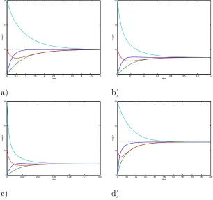
align their paths according the formation center at time 0 that we assume expressed as the generic agreement function of the initial UAVs heights. In particular, in the four simulated vertical alignment maneuvers, the position of the formation center is defined respectively as the i) arithmetic mean, ii) geometric mean, iii) harmonic mean, iv) mean of order 2 of the initial positions of all UAVs. The initial height isx(0) = (5,5,10,20)T. We stress once again that the challenging aspect is that the UAVs know the heights of only their neighbors and are required to align their paths according to the path of the formation center, which in turns depend on the unknown position of all UAVs.
In case i), (see e.g., [1,3,13]) the UAVs are given an individual objective (3) with penalty
F(xi, x(i)) =
P
j∈Ni(xj −xi)
2
and consequently implement the optimal linear protocol
u(xi, x(i)) =
X
j∈Ni
to asymptotically align on the arithmetic mean ofx(0). Notice that, the approximate objective function (13) converges even if the neighbors are not aligned, since both the above integrand penalty F(xi,x¯(i)) and the control (28) are null when xi is equal to the arithmetic mean computed over the only neighbors’ states. Figure 2 a) shows the simulation of the longitudinal flight dynamics.
In case ii) the UAVs are given an individual objective F(xi, x(i)) =
xiPj∈Ni(xj−xi)
2
and
0 0.5 1 1.5 2 2.5 3 3.5 4 4.5 5
5 10 15 20
time
height
0 0.1 0.2 0.3 0.4 0.5 0.6 0.7
5 10 15 20
time
height
a) b)
0 0.02 0.04 0.06 0.08 0.1 0.12
5 10 15 20
time
height
0 20 40 60 80 100 120 140 160 180 200 5
10 15 20
time
height
[image:17.612.142.448.171.458.2]c) d)
Fig. 2. Longitudinal flight dynamics converging to a) the arithmetic mean under protocol (28); b) the geometric mean under protocol (29); c) the harmonic mean under protocol (30); d) the mean of order 2 under protocol (31).
implement the optimal protocol
u(xi, x(i)) =xi
X
j∈Ni
(xj −xi) (29)
to asymptotically align on the geometric mean of x(0). Figure 2 b) shows the simulation of the longitudinal flight dynamics.
In case iii) the UAVs are given an objective function F(xi, x(i)) =
x2
i
P
j∈Ni(xj−xi)
2
and implement the optimal protocol
u(xi, x(i)) =−x2i
X
j∈Ni
to asymptotically align on the harmonic mean of x(0). Figure 2 c) shows the simulation of the longitudinal flight dynamics.
Finally, in case iv) the UAVs are given a function F(xi, x(i)) =
1 2xi
P
j∈Ni(xj−xi)
2
and implement the optimal protocol
u(xi, x(i)) =
1 2xi
X
j∈Ni
(xj−xi) (31)
to asymptotically align on the mean of order 2 of x(0). Figure 2 d) shows the simulation of the longitudinal flight dynamics.
Protocols (28)-(31) are characterized by different converging times (see Figs. 2). These dif-ferences are due to the fact that the protocols multiply the common term P
j∈Ni(xj −xi)
for different powers of xi, respectively 1, xi, −x2i and 21x−i 1. Being xi ≥ 1 for all i ∈ Γ and
t ≥0, the lower the power, the higher the converging time. Consider the vertical alignment to the mean of power 2. To obtain a converging time comparable with the one of the vertical alignment to the arithmetic mean, we modify the protocol so that it turns to be a ratio between polynomials whose numerator is of an order greater than the denominator as in the arithmetic mean case. As an example, in Fig. 3 a) results are reported with the protocol (31) modified as
u(xi, x(i)) =
1 2xi
X
j∈Ni
(x2j −x2i). (32)
An analogous result can be obtained if we multiply the protocol (31) by twice an upper bound of maxi∈Γ{xi(0)}. The resulting scaled protocol is
u(xi, x(i)) =
maxi∈Γ{xi(0)} 2xi
X
j∈Ni
(xj −xi) (33)
and the corresponding longitudinal dynamics is displayed in Fig. 3 b). Unfortunately both protocols (32) and (33) have some drawbacks. In (32), the functionϑ(xi) =x2i is not concave, whereas to implement protocol (33) the UAVs must have an a-priori knowledge or at least a bound of maxi∈Γ{xi(0)}.
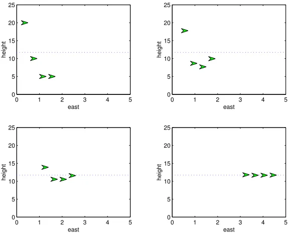
An example of vertical alignment maneuver under protocol (33) is displayed in Fig. 4.
7 Conclusions and Discussion
0 0.5 1 1.5 2 2.5 3 3.5 4 4.5 5 5
10 15 20
time
height
0 0.5 1 1.5 2 2.5 3 3.5 4 4.5 5
5 10 15 20
time
height
[image:19.612.145.447.55.202.2]a) b)
Fig. 3. Longitudinal flight dynamics converging to the mean of order 2: a) under protocol (32); b) under protocol (33).
0 1 2 3 4 5
0 5 10 15 20 25
height
east
0 1 2 3 4 5
0 5 10 15 20 25
height
east
0 1 2 3 4 5
0 5 10 15 20 25
height
east
0 1 2 3 4 5
0 5 10 15 20 25
height
east
Fig. 4. Vertical alignment to the mean of order 2 on the vertical plane.
stationary linear or non-linear protocol, provided that the networks defined by the communi-cation links between agents is time-invariant and connected Also, we have proposed a game theoretic approach to solve consensus problems. Under this perspective, consensus is the re-sult of a mechanism design. A supervisor imposes individual objectives. Then, the agents reach asymptotically consensus as a side effect of the optimization of their own individual objectives on a local basis.
Among the limitations of Assumption 1 on the structure of function ˆχ(x) = f(P
[image:19.612.152.441.255.488.2]If we consider a more general function gi(x,x(i)) for each agent, following a line of rea-soning as in Section 3, we can prove that, e.g., a protocol with component ui(x,x(i)) =
1
P
j∈Ni∪{i}∂xj∂gi
P
j∈Ni(xj−xi), for all i∈ Γ, leaves the value ˆχ(x) time-invariant. Also, we can
show that the same protocol makes the agents asymptotically converge to the group decision value if ∂gi
∂xj >0, for all j ∈Ni∪ {i}. However, in this case, we are able to prove the analogous
of Theorem 2 only making use of a Lyapunov function that takes into account of the struc-ture of the network G. Hence, the proof of convergence is not generalizable to networks with switching topology. This last negative result should not surprise as, in case of a switching topology, functionsgi(.) should be redefined at each switching instant as they are defined not only on the value of xi but also on the value ofx(i) and hence they depend on the topology of the network G.
As an example, consider a system withxi(0)>0, for alli∈Γ, for which the desired consensus value is ˆχ(x(0)) = 1
n
P
i∈ΓPj∈Niaij q
xi(0)xj(0) where aij > 0 and Pj∈Niaij = 1, for all
i∈Γ, j∈Ni. Then a possible consensus protocol on a fixed network is ui = 2
P
j∈Ni(xj−xi)
P
j∈Ni
qxi
xj+
xj xi
.
References
[1] R. Olfati-Saber, R. Murray, Consensus problems in networks of agents with switching topology and time-delays, IEEE Transactions on Automatic Control 49 (9) (2004) 1520–1533.
[2] W. Ren, R. Beard, E. M. Atkins, A survey of consensus problems in multi-agent coordination, in: Proc. of the American Control Conference, Portland, OR, USA, 2005, pp. 1859–1864.
[3] D. Bauso, L. Giarr´e, R. Pesenti, Attitude Alignment of a Team of UAVs under Decentralized Information Structure, in: Proc. of the IEEE Conference on Controls and Applications, Instanbul, Turkey, 2003, pp. 486–491.
[4] F. Giulietti, L. Pollini, M. Innocenti, Autonomous Formation Flight, IEEE Control Systems Magazine 20 (2000) 34–44.
[5] R. W. Beard, T. W. McLain, M. A. Goodrich, E. P. Anderson, Coordinated Target Assignment and Intercept for Unmanned Air Vehicles, IEEE Transactions on Robotics and Automation 18 (6) (2002) 911–922.
[6] H. G. Tanner, A. Jadbabaie, G. J. Pappas, Stable flocking of mobile agents, part i: Fixed topology, in: Proc. of the 42th IEEE Conference on Decision and Control, Maui, Hawaii, 2003, pp. 2010–2015.
[7] V. Gazi, K. Passino, Stability analysis of social foraging swarms, IEEE Trans. on Systems, Man, and Cybernetics 34 (1) (2004) 539–557.
[8] Y. Liu, K. Passino, Stable social foraging swarms in a noisy environment, IEEE Transactions on Automatic Control 49 (1) (2004) 30–44.
[10] D. Bauso, L. Giarr´e, R. Pesenti, Neuro-dynamic programming for cooperative inventory control, in: Proc. of the American Control Conference, Boston, Ma, 2004, pp. 5527–5532.
[11] A. J. Kleywegt, V. S. Nori, M. W. P. Savelsbergh, The Stochastic Inventory Routing Problem with Direct Deliveries, Transportation Science 36 (1) (2002) 94–118.
[12] S. H. Low, F. Paganini, J. C. Doyle, Internet Congestion Control, IEEE Control System Magazine 22 (1) (2002) 28–43.
[13] R. Olfati-Saber, R. Murray, Consensus protocols for networks of dynamic agents, in: Proc. of the American Control Conference, Vol. 2, Denver, Colorado, 2003, pp. 951–956.
[14] A. Fax, R. M. Murray, Information flow and cooperative control of vehicle formations, IEEE Transactions on Automatic Control 49 (9) (2004) 1565–1476.
[15] A. Jadbabaie, J. Lin, A. Morse, Coordination of Groups of mobile autonomous agents using nearest neighbor rules, IEEE Transactions on Automatic Control 48 (6) (2003) 988–1001.
[16] L. Moreau, Leaderless coordination via bidirectional and unidirectional time-dependent communication, in: Proc. of the 42nd IEEE Conference on Decision and Control, Maui, Hawaii, 2003, pp. 3070–3075.
[17] W. Ren, R. Beard, Consensus of information under dynamically changing interaction topologies, in: Proc. of the American Control Conference, Vol. 6, Boston, Massachussets, 2004, pp. 4939– 4944.
[18] W. Ren, R. Beard, Consensus seeking in multi-agent systems under dynamically changing interaction topologies, IEEE Transactions on Automatic Control 50 (5) (2005) 655–661.
[19] H. G. Tanner, A. Jadbabaie, G. J. Pappas, Stable flocking of mobile agents, part ii: Dynamic topology, in: Proc. of the 42th IEEE Conference on Decision and Control, Maui, Hawaii, 2003, pp. 2016–2021.
[20] T. W. McLain, R. W. Beard, Coordination Variables Coordination Functions and Coooperative Timing Missions, in: Proc. of the IEEE American Control Conference, Denver, Colorado, 2003, pp. 296–301.
[21] W. Ren, R. Beard, T. McLain, Coordination variables and consensus building in multiple vehicle systems, in: Proc. of the Block Island Workshop on Cooperative Control, Lecture Notes in Control and Information Sciences series, Vol. 309, Springer-Verlag, 2004, pp. 171–188.
[22] L. Xiao, S. Boyd, Fast linear iterations for distributed averaging, Systems and Control Letters 53 (1) (2004) 65–78.
[23] T. Basar, G. Olsder, Dynamic Noncooperative Game Theory, Academic Press, London, 1995, 2nd ed.
[24] P. Cardaliaguet, S. Plaskacz, Invariant solutions of differential games and Hamilton–Jacobi– Isaacs equations for time-measurable Hamiltonians, SIAM Journal on Control and Optimization 38 (5) (2000) 1501–1520.
[25] M. J. Osborne, A. Rubinstein, A Course in Game Theory, MIT press, Cambridge, MA, 1994.
[27] W. B. Dunbar, R. M. Murray, Distributed Receding Horizon Control with Application to Multi-Vehicle Formation Stabilization, Automatica. To appear.
[28] W. B. Dunbar, R. M. Murray, Receding Horizon Control of Multi-Vehicle Formations: A Distributed Implementation, in: Proc. of the 43rd IEEE Conference on Decision and Control, Vol. 2, Paradise Island, Bahamas, Dec., 2004, pp. 1995–2002.
[29] W. Li, C. G. Cassandras, A cooperative receding horizon controller for multivehicle uncertain environments, IEEE Transactions on Automatic Control 51 (2) (2006) 242–257.
[30] E. Franco, T. Parisini, M. M. Policarpou, Cooperative control of distributed agents with nonlinear dynamics and delayed information exchange: a stabilizing receding-horizon approach, in: 44th IEEE CDC-ECC, Seville, Spain, 2005, pp. 2206–2211.
[31] D. Bauso, L. Giarr´e, R. Pesenti, Mechanism design for optimal consensus problems, DINFO Technical report 3/06, Submitted to CDC.