Two-Host, Two-Vector Basic Reproduction Ratio (R-0) for Bluetongue

Bluetongue

Joanne Turner1*, Roger G. Bowers2, Matthew Baylis1

1Department of Epidemiology and Population Health, Institute of Infection and Global Health, University of Liverpool, Leahurst, Neston, United Kingdom,2Department of Mathematical Sciences, School of Physical Sciences, University of Liverpool, Liverpool, United Kingdom

Abstract

Mathematical formulations for the basic reproduction ratio (R0) exist for several vector-borne diseases. Generally, these are based on models of one-host, one-vector systems or two-host, one-vector systems. For many vector borne diseases, however, two or more vector species often co-occur and, therefore, there is a need for more complex formulations. Here we derive a two-host, two-vector formulation for theR0of bluetongue, a vector-borne infection of ruminants that can have serious economic consequences; since 1998 for example, it has led to the deaths of well over 1 million sheep in Europe alone. We illustrate our results by considering the situation in South Africa, where there are two major hosts (sheep, cattle) and two vector species with differing ecologies and competencies as vectors, for which good data exist. We investigate the effects onR0of differences in vector abundance, vector competence and vector host preference between vector species. Our results indicate thatR0can be underestimated if we assume that there is only one vector transmitting the infection (when there are in fact two or more) and/or vector host preferences are overlooked (unless the preferred host is less beneficial or more abundant). The two-host, one-vector formula provides a good approximation when the level of cross-infection between vector species is very small. As this approaches the level of intraspecies cross-infection, a combination of the two-host, one-vectorR0for each vector species becomes a better estimate. Otherwise, particularly when the level of cross-infection is high, the two-host, two-vector formula is required for accurate estimation ofR0. Our results are equally relevant to Europe, where at least two vector species, which co-occur in parts of the south, have been implicated in the recent epizootic of bluetongue.

Citation:Turner J, Bowers RG, Baylis M (2013) Two-Host, Two-Vector Basic Reproduction Ratio (R0) for Bluetongue. PLoS ONE 8(1): e53128. doi:10.1371/ journal.pone.0053128

Editor:Jesus Gomez-Gardenes, Universidad de Zarazoga, Spain

ReceivedSeptember 7, 2012;AcceptedNovember 26, 2012;PublishedJanuary 8, 2013

Copyright:ß2013 Turner et al. This is an open-access article distributed under the terms of the Creative Commons Attribution License, which permits unrestricted use, distribution, and reproduction in any medium, provided the original author and source are credited.

Funding:This work was funded by The Leverhulme Trust (http://www.leverhulme.ac.uk) through Research Leadership Award F/0025/AC ‘‘Predicting the effects of climate change on infectious diseases of animals’’, which was awarded to Matthew Baylis. The funder had no role in study design, data collection and analysis, decision to publish, or preparation of the manuscript.

Competing Interests:The authors have declared that no competing interests exist.

* E-mail: [email protected]

Introduction

Mathematical formulations for the basic reproduction ratio (R0) – defined as the average number of secondary infections produced by a typical primary infection in an otherwise totally susceptible population [1] – exist for several vector-borne diseases including those with one host and one vector, such as malaria [2] and those with two hosts and one vector, such as zoonotic trypanosomiasis [3], African horse sickness [4] and bluetongue [5,6]. To date, with the exception of Lopez et al. [7], almost no attention has been paid

to developing mathematical formulations ofR0 where there are

both multiple hosts and multiple vectors. However, this is a common situation: for trypanosomiasis in Africa for example, two or more species of tsetse fly vector often co-exist; while for both African horse sickness and bluetongue in southern Africa, two competent vectors (Culicoides imicolaandC. bolitinos) are frequently trapped together. Other diseases transmitted by multiple vectors include dengue [8], Japanese encephalitis [9] and malaria [10].

This situation may also apply to the recent European outbreak of bluetongue, which has caused the deaths of well over a million sheep. The outbreak began in 1998 in regions of southern Europe where the Afrotropical midge,C. imicola, occurs. Starting in 1999, it was also detected in Balkan countries whereC. imicolawas not

known, thereby implicating local Culicoides species, such as the obsoletusandpulicarisgroups, as vectors. Since these co-occur with C. imicolaover the latter’s European range [11], it was reasonable to suspect that they may transmit the virus alongsideC. imicolain some places; and epidemiological evidence for this was later provided in Sicily [12]. Subsequently, both BTV 1 and BTV 8 have been transmitted in regions with indigenous vectors, both with and withoutC. imicola. It is therefore quite likely that two or more vector species have co-transmitted BT virus in several parts of Europe in recent years.

competence and also varies with species and temperature [15]; (3) vector host preference, which differs between species [14,16,17].

Importantly, we also work directly with R0, rather than the

thresholdTproposed by Lopez et al. [7], which is not valid in all

regions of feasible parameter space. The notation we use allows us to make direct comparisons with a previously published two-host, one-vector formula for bluetongue. We illustrate our results by parameterising the model for a specific disease system, namely

Table 1.Definitions and descriptions of the variables, parameters and rates that influence the dynamics of the host, two-vector system and the parameter values used to estimateR0.

Variable, Parameter

or Rate Construction Definition or Description

Point Estimate and/or Feasible Range

Comments and Formula if Temperature-dependent [vector species]

xi

Xi

/Hi proportion of host typeithat are susceptible ican beC(cattle) orS(sheep) yi

Yi

/Hi proportion of host typeithat are infectious zi

Zi

/Hi proportion of host typeithat have recovered

Hi X

i

+Yi+Zi total number of host typei

lHi lHi~ P

j~f1,2g

bjajwijmijIj=Nj rate at which susceptible hosts of typei

become infectious through being bitten by infectious vectors

jcan be 1 (C. imicola) or 2 (C. bolitinos)

bj probability of transmission from vector typej

to a host given an effective contact

0.8–1.0 [C. sonorensis]

aj biting rate of vector typej 0–0.5 a(T)~0:0002T(T{3:7)(41:9{T)1=2:7

[C. sonorensis]

wij wCj~_HCjHCjzsjHSj~ mSj mSjzsjmCj wSj~1{wCj

proportion of vectors of typejattracted to hosts of typei

As Gubbins et al. [6], for clarity we replacewCjandwSjwithwjand1{wj

respectively.

sj host preference of vector typej

s,1 indicates a preference for cattle

s.1 indicates a preference for sheep

0–1 C. imicolafeeds predominantly on cattle and sheep [16,17], but prefers cattle [23].

C. bolitinosfeeds on cattle and horses [16,17] and breeds in cattle dung [14].

mij Nj/Hi ratio of vectors of typejto hosts of typei Many areas: mC1=mS1= 500

(0–5000)

mC2=mS2= 50

(0–500) Colder high-lying areas:

mC1=mS1= 50

(0–100)

mC2=mS2= 500

(0–5000)

In general,C. imicolais approx. 10 times more abundant thanC. bolitinos[15]. In colder, high-lying areas,C. imicolais approx. 10 times less abundant than

C. bolitinos[14].

Nj Sj+Lj+Ij total number of vectors of typej

ri recovery rate of host typei rC= 1/20.6

rS= 1/16.4 di pathogen-induced mortality rate of host typei dC= 0

dS= 0.001–0.01 Sj number of vectors of typejthat are susceptible

Lj number of vectors of typejthat are latent

Ij number of vectors of typejthat are infectious

lVj lVj~ P

i~fC,Sg

bjajwijyi rate at which susceptible vectors of typej

become latent through biting infectious hosts

bj probability of transmission from a host to

vector typejgiven an effective contact

b1= 0.0021–0.0654

b2= 0.0268–0.6444

b1(T)~0:0003699 exp(0:1725T)

[C. imicola]

b2(T)~0:005465 exp(0:159T)

[C. bolitinos] Both from data in [15].

nj rate at which latent vectors of typejbecome

infectious ( = 1/EIP, where EIP = extrinsic incubation period)

1/4–1/26 v(T)~0:0003T(T{10:4)

[C. sonorensis]

mj natural mortality rate of vector typej 0.1–0.5 m(T)~0:009 exp(0:16T)

[C. sonorensis]

rj replacement rate of vector typej

bluetongue in South Africa. We use the situation in South Africa because of the availability of extensive distribution data, together with detailed experimental results on the relative vector compe-tencies of the two main vector species [15]. Similar data for different European bluetongue vectors do not exist. It is known that several European vector species transmit bluetongue virus and that there are differences in host preference between these species. For example, Garros et al. [18] show thatC. chiopterusprefers to feed on cattle whileC. obsoletusis more of a generalist. However, nothing is known of their respective vector competencies. This highlights the need for a two-host, two-vector formula forR0as well as experimental work to establish the vector competence of each species. Although we have focussed on the situation in South Africa, the framework and general results presented here are equally relevant to Europe.

Analysis

Model Equations

Equations describing the dynamics of a two-host, two-vector system are given below, whilst the variables and parameters of the model are defined and described in Table 1. For clarity, we have adopted a similar notation to that used by Gubbins et al. [6]. In short, hosts can be either susceptible, infectious or recovered (and in this case immune), whilst vectors can be either susceptible, latent or infectious. The proportions of susceptible, infectious and recovered hosts are denoted byxi_,yi_andzi_{respectively, whilst the}

numbers of susceptible, latent and infectious vectors are denoted bySj,LjandIjrespectively (Njin total). Susceptible hosts of typei

[whereican be eitherC(cattle) orS(sheep)] become infectious at ratelHi, which is the sum over vector types indicated byj[wherej can be either 1 (C. imicola) or 2 (C. bolitinos)] of bjaj(wijmijIj=Nj).

The third term is composed ofmij the ratio of vectors of typejto

hosts of typei,IjNj the proportion of vectors of typejthat are

infectious andw_ij the proportion of vectors of typejattracted to hosts of typei(i.e. reflecting the preference of vector typejfor host typei). So, the third term gives the average number of infectious vectors of type j attracted to a host of type i (after taking into account vector typej’s preference for host typei). This is multiplied byaj, the (temperature-dependent) biting rate of vectors of typej,

andbj, the probability of transmission from a vector of typejto a

host given an effective contact. Similarly, susceptible vectors of typejbecome latent at ratelVj, which is the sum over host types (indicated byi) ofb_jaj(wijyi). The third term is the probability of a

vector of typejbeing attracted to an infectious host of typei. This is multiplied by aj, the (temperature-dependent) biting rate of

vectors of typej, andb_j, the probability of transmission from a host to a vector of typejgiven an effective contact. An infectious host remains infectious until it either recovers (at rateri) or dies (at rate di). After a short extrinsic incubation period (on average 1/nj), latent vectors become infectious. They remain infectious until they die, which occurs at ratem_j. Susceptible vectors are added to the system at rate r_j. The model assumes that there is no seasonal aspect to vector recruitment or population size and that there is no latent period in hosts, recovered animals are immune and the host population remains constant except for losses due to disease-induced mortality.

Hosts.

dxi

dt ~{lHix

i

dyi

dt~lHix

i_{(r izdi)yi

dzi

dt~riy

i

wherei[fC,Sg. Vectors.

dSj

dt ~rjNj{lVjSj{mjSj

dLj

dt ~lVjSj{(njzmj)Lj

dIj

dt~njLj{mjIj

wherej[f1,2g.

Basic Reproduction Ratio

The ability of the pathogen to spread can be expressed in terms

of the basic reproduction ratio R0. Mathematically, R0 is the

dominant eigenvalue of the next-generation matrixK. For vector-borne transmission models like the one described above,

K~ 0 A B 0

where matrixAdescribes vector to host transmission and matrixB describes host to vector transmission (see Appendix 1 in File S1). We could work directly with the characteristic equation

DK{lID~0. However, there are significant advantages in using

a result shown in Appendix 2 in File S1, namely thatR0is the

square root of the dominant eigenvalue ofBA(a 464 submatrix of K2). Not only isBAsmaller thanKbut also its elements have an obvious biological interpretation in terms of Rij, the average number of infectious vectors of typeiproduced by one infectious vector of typej(necessarily in two generations). It is such biological

interpretation that we seek. The utility of working with BA is

doubtless associated with the argument that, in contrast to directly-transmitted infections, for vector-borne infectionsR2

0makes more

sense biologically [2] and is in fact what is measured in the field (i.e. two-generation ‘like’ to ‘like’ transmission).

Following the above procedure we find that

R0~

ffiffiffiffiffiffiffiffiffiffiffiffiffiffiffiffiffiffiffiffiffiffiffiffiffiffiffiffiffiffiffiffiffiffiffiffiffiffiffiffiffiffiffiffiffiffiffiffiffiffiffiffiffiffiffiffiffiffiffiffiffiffiffiffiffiffiffiffiffiffiffiffiffiffiffiffiffiffiffiffiffiffiffiffiffiffiffiffiffiffiffiffiffiffiffiffiffiffiffiffiffiffiffiffiffiffi

1

2½(R11zR22)z

ffiffiffiffiffiffiffiffiffiffiffiffiffiffiffiffiffiffiffiffiffiffiffiffiffiffiffiffiffiffiffiffiffiffiffiffiffiffiffiffiffiffiffiffiffiffiffiffiffiffiffiffiffiffiffiffiffiffiffiffiffiffiffiffiffiffiffiffi

(R11zR22)2{4(R11R22{R12R21) q

r

,ð1Þ

where specifically

R11~

b1b1a21

m₁

_n

1

n1zm1

_w2

1mC1

rCzdC

z(1{w1)

2_m S1

rSzdS !

R22~

b2b2a22

m₂

n2

n2zm2

w2₂mC2

rCzdC

z(1{w2)

2_m S2

rSzdS !

R12~

b2b1a2a1

m₂

_n

2

n2zm2

_w

2w1mC1

rCzdC

z(1{w2)(1{w1)mS1 rSzdS

R21~

b1b2a1a2

m₁

_n

1

n1zm1

_w

1w2mC2

rCzdC

z(1{w1)(1{w2)mS2 rSzdS

Note that the proportion of vectors of typejattracted to hosts of typei

w_ij~_PvijHi

kvkjHk

,

wherevijis a measure of vector typej’s preference for host typei

andHiis the total number of hosts of typei. For two host species

(cattleCand sheepS), this can be rewritten as

w_Cj~ HC HCzsjHS

andw_Sj~1{w_Cj,

where vector host preference is now denoted by sj. In terms of

vector to host ratios, wheremCj~Nj=HC and mSj~Nj=HS, the

first of these is

w_Cj~ mSj mSjzsjmCj

: ð3Þ

As Gubbins et al. [6], for clarity we replacew_Cj andw_Sj withw_j

and1{w_jrespectively.

From Gubbins et al. [6], we know that R0~ ffiffiffiffiffiffiffiffiR11

p and

R0~ ffiffiffiffiffiffiffiffiR22

p

for two-host, one-vector systems involving vector type 1 and vector type 2, respectively. For the two-host, two-vector

system we find from equations (2) that when w₁~w₂,

R11R22{R12R21~0 and hence R0~ ffiffiffiffiffiffiffiffiffiffiffiffiffiffiffiffiffiffiffiR11zR22

p

. If vectors 1 and 2 are identical in terms of parameter values (i.e. all parameter values for vector species 1 equal those for vector species 2) and equal in number, thenR11~R22~R12~R21and soR0~ ffiffiffiffiffiffiffiffiffiffi2R11

p . In other words, the two-host, two-vector R0 is greater than the

two-host, one-vectorR0 by a factor of ffiffiffi

2 p

. So, in this case, if it were assumed that there was only one vector species transmitting the infection, the basic reproduction ratio would be underesti-mated (because the average number of relevant vectors per host would be underestimated). When the vectors are not identical, as the level of cross-infection_{ffiffiffiffiffiffiffiffi} R12R21 increases, R0 increases from

R11

p

(when R12R21~0 and R11wR_{22), through} ffiffiffiffiffiffiffiffiffiffiffiffiffiffiffiffiffiffiffiR₁₁zR₂₂ p

(when R11R22{R12R21~0) to 4ffiffiffiffiffiffiffiffiffiffiffiffiffiffiffiR12R21

p

(when R12R21 is very

large).

Results

For the two-host, one-vector system, Gubbins et al. [6] found

that the parameters with a significant effect on R0 were

temperature (T) [via biting rate, extrinsic incubation period

(EIP), vector mortality rate], the probability of transmission from

host to vector (b) [which was not temperature-dependent in

Gubbins et al. [6]] and the ratios of vectors to hosts (mCandmS).

For the two-host, two-vector system, we propose to focus on the effects onR0of varying the ratios of vectors to hosts (mC1,mC2,mS1, mS2) [linked to vector abundance], the probabilities of transmission from host to vector (b1, b2) [linked to vector competence and temperature-dependent in our model] and the vector host preferences (s1,s2). Our aim is to provide a general framework for two-host, two-vector approaches to bluetongue; however there is a paucity of data. There is one situation, South Africa, whereC. imicolaandC. bolitinoscoexist across most of the country and for which we do have data. We undertake the analysis with reference to this.

As shown by Meiswinkel et al. [13], there are many areas (e.g. Western Cape, western part of the Eastern Cape, Mpumalanga,

Gauteng and Limpopo Province) where C. imicola is 10 to 100

times more abundant thanC. bolitinos. However, there are areas, in particular in the cooler high-lying areas of the Free State, whereC. bolitinosis approximately 10 times more abundant thanC. imicola [14] and Venter et al. [19] suggest thatC. bolitinosmay play an important role in the transmission of BTV in these areas. Paweska et al. [15] demonstrate that, regardless of incubation temperature (10, 15, 18, 23.5 or 30uC), the mean virus titre/midge, infection rate and proportion of infected females with transmission potential (i.e. virus titre/midge$103TCID50, where TCID50(tissue culture infectious dose 50) is the amount of virus that will infect 50% of midges inoculated with it) are significantly higher in C. bolitinos than in C. imicola and suggest that, because of its significantly higher vector competence,C. bolitinoscould be the primary vector in areas where it occurs inlowernumbers thanC. imicola, as well as in these cooler regions. Here, abundance is expressed through the ratios of vectors to hosts (mC1, mC2, mS1, mS2), while vector competence is expressed through the probabilities of transmission from host to vector (b1, b2). Regarding vector host preferences, there is evidence [14,16] that manyCulicoidesspecies prefer to feed

on cattle and some suggestion thatC. bolitinos may not feed on

sheep at all [16,17].

Estimatingb1andb2

Fu et al. [20] show that only midges containing$103TCID50

release detectable amounts of virus in their saliva. So, first we define ‘infectious’ as ‘having a virus titre$103TCID50’. Next we obtain from Table 2 of Paweska et al. [15], for several different temperatures, the proportion of vectors remaining that are infectious [i.e. (number of infectious vectors)/(number of initially susceptible vectors known to have fed on infected blood and still be alive after the incubation period)]. Each of these data points is equal tobjat a given temperature. By fitting curves to the data, we can find temperature-dependent functions forb1(C. imicola) andb2 (C. bolitinos). Exponential curves of the formb_j~pjexp(qjT)were

fitted using a nonlinear least-squares method with bisquare weighting of the residuals. The coefficients and goodness of fit statistics are given in Table 2. The curves (shown in Appendix 3 in File S1) adequately describe the relationships betweenb1,b2and temperature over this range of temperatures. Note that as temperature varies from 10 to 30uC, the ratiob2/b1varies from 9.85 to 12.91 (i.e. the probability of transmission ofC. bolitinosis always about 10 times greater than that ofC. imicola).

Other parameter estimates

taken from Gubbins et al. [6]. Details are given in Table 1. Six of these estimates aj, nj and mj (i.e. three for each vector species) depend on temperature. They are positive and increase mono-tonically for temperatures between 10.4uC and 35.5uC.

Effect of differences inmijandbj

In order to focus on the effects onR0of differences in vector competence, vector abundance and vector host preference, the two species of vectors are assumed to be the same in every way exceptbj,mijandsj. We first consider the effect of differences inmij for fixedbjandsj.

First note that, as shown in equation (3),wCjvaries withmCj,mSj andsj. However, whenmCjequalsmSj,wCj(and hencewj) depends onsjalone. In Figure 1 (and Figure 2 below),mS1andmS2equal mC1andmC2respectively ands1=s2= 0.5. Consequentlyw1and

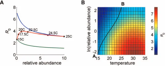
w2are fixed at 0.67. The transmission probabilitiesb1andb2are determined (as described in Table 1) by temperature, which is 25uC in Figure 1A and 15uC in Figure 1B. The parametersmC1 andmC2vary independently along thexandyaxes respectively. In Figure 1A, we can clearly see thatR0is greater when vector 2 (C. bolitinos) is more abundant than vector 1 (C. imicola) [i.e. whenmC2 is greater thanmC1] than when the reverse is true. For example, whenmC1= 50 andmC2= 500 (i.e. in the top left-hand corner),R0 is 7.0, whereas, whenmC1= 500 andmC2= 50 (i.e. in the bottom right-hand corner),R0is only 3.1. This large difference is due to the fact that b2 is approximately 10 times greater than b1 and illustrates the balance between vector abundance and vector competence forC. imicolaandC. bolitinos. The same relationship is observed when the temperature is 15uC (i.e. in Figure 1B), butR0 is much smaller at this temperature.

It is also clear from Figure 1 that omitting one vector species (i.e. being constrained to one axis) leads to underestimation ofR0and when that species has a significantly higher vector competence (as does vector species 2) the degree of underestimation can be dramatic.

In Figure 2,b1and b2vary with temperature, as described in Table 1. The vector to host ratiosmS1andmS2equalmC1andmC2 respectively, which vary simultaneously withxas described below:

mC1~500{450x

mC2~50z450x

for 0ƒxƒ1:

Relative abundance (mC1/mC2=N1/N2) is therefore described by

the hyperbola

mC1

mC2

~ 550

50z450x{1:

Figure 2A shows howR0varies with relative abundance. Curves 1 (green) and 2 (blue) show the relationship when temperature is fixed at 15uC and 25uC, respectively. Curve 3 (red) is produced

when temperature (T~25{10x for 0ƒxƒ1) and relative

abundance vary simultaneously with x. Hence, curve 3 (red)

shows the relationship when temperature varies from 15uC to

25uC as relative abundance varies from 0.1 (whenC. bolitinosis 10 times more abundant thanC. imicola) to 10 (whenC. imicolais 10 times more abundant thanC. bolitinos). By definition, curve 3 is constrained to start at the same point as curve 1 and end at the same point as curve 2. Curve 3 can be thought of as a path across the landscape, moving from the cooler high-lying regions whereC. bolitinosdominates to the warmer low-lying regions whereC. imicola

dominates. Along this path, temperature (and hence bj) and

relative abundance vary simultaneously.

Figure 2B shows howR0varies with relative abundance (y axis) and temperature (x axis) separately. It clearly shows that, for a fixed temperature,R0always decreases as relative abundance ofC. imicolaincreases. It also shows that, for fixed relative abundance, R0initially increases with temperature, but starts to decrease again

beyond 31uC. Curve 3 in Figure 2A corresponds to moving from

A to B across the surface in Figure 2B. Along this path, the highest R0corresponds to a relative abundance of approximately 1.4 and a temperature of approximately 21.1uC. In this case, for

tempera-tures greater than 21.1uC, R0 drops with rising temperature

because, at the same time, the less competent vector is replacing the more competent one.

In summary, we find that high vector competence can compensate for low vector abundance and that temperature, which determines the transmission probabilitiesb1andb2and also influences the abundance and composition of vector species, has a marked effect onR0.

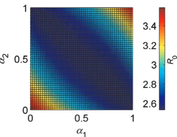
Effect of differences insj

We now consider the important effect that vector host preference (sj) has onR0. In order to focus on the effect ofsj, we assume that the vector species differ only insj. Also, to ensure that there is no advantage to choosing cattle over sheep (or vice versa), we set rC=rS, dC=dS and mC1=mS1=mC2=mS2. When

sj= 0, the proportion of vectors of type j attracted to cattle (wj)

equals 1. Whensj= 1 (i.e. no preference),wj just depends on the

relative numbers of each host species, with a greater number resulting in a greater share of the vectors. AssjR‘,wjR0 where

all vectors are attracted to sheep. To prevent loss of detail as

sjR‘, in Figure 3 we use aj rather than sj, where aj is an

alternative measure of vector host preference such that

sj~aj=(1{aj). From this formula we can see that as aj varies from 0 to 1,sjvaries from 0 to‘and thataj= 0.5 indicates no preference.

Figure 3 clearly shows that the minimum value ofR0lies on a straight line running from (a1= 0,a2= 1), wherew1~1andw2~0

(i.e. vector type 1 feeds exclusively on cattle while vector type 2 feeds exclusively on sheep), through (a1= 0.5, a2= 0.5), where w₁~0:5andw₂~0:5(i.e. neither vector has a preference and so both vector species are equally distributed between both host species), to (a1= 1,a2= 0), wherew1~0andw2~1(i.e. vector 1

feeds exclusively on sheep while vector 2 feeds exclusively on

Table 2.Coefficients and goodness of fit statistics for exponential curves of the formb_j~pjexp(qjT), wherejcan

be 1 (C. imicola) or 2 (C. bolitinos), fitted to data extracted from Paweska et al. [15].

C. imicola C. bolitinos

Coefficients (with 95% confidence bounds)

p 0.0003699

(20.0002815, 0.001021)

0.005465 (20.0162, 0.02713)

q 0.1725

(0.1111, 0.2339)

0.159

(0.01987, 0.2982)

Goodness of fit

sse 8.5345e-005 0.0519

adjrsquare 0.9648 0.8578

rmse 0.0046 0.1139

cattle). Any deviation from this line results in a higherR0. This figure clearly shows two things: firstly, that different combinations of vector host preferences can result in the sameR0; second, that when both vectors prefer the same host species,R0is greater. This result is important because it shows that, when the vector species differ only in host preference and the host species are equally good as hosts (in this case, they share the same infectious period and the same pathogen-induced mortality rate) and equally abundant, overlooking vector host preference can result in an underestima-tion ofR0.

In Figures 1 and 2 and Table 3, we useds1=s2= 0.5 (which

corresponds toa1=a2= 1/3) as manyCulicoidesspecies prefer to

feed on cattle [14,16]. However, while it is clear thatC. imicolaalso feeds on sheep (and even horses and pigs too), there is some evidence thatC. bolitinosdoes not – instead feeding exclusively on cattle and horses [16,17]. A strong association betweenC. bolitinos and cattle is further suggested by the fact thatC. bolitinosbreeds in cattle dung [14], rather than soil likeC. imicola. In terms ofR0, ifC. bolitinos does not feed on sheep, thens2= 0 (i.e. a2= 0) and the

true value of R0 will be higher than our estimates based on

s2= 0.5.

R0approximations

The need for the two-host, two-vector formula is further emphasised when we consider several approximations based on

the two-host, one-vector formula forR0, which is

R0~

ffiffiffiffiffiffiffiffiffiffiffiffiffiffiffiffiffiffiffiffiffiffiffiffiffiffiffiffiffiffiffiffiffiffiffiffiffiffiffiffiffiffiffiffiffiffiffiffiffiffiffiffiffiffiffiffiffiffiffiffiffiffiffiffiffiffiffiffiffiffiffiffiffiffiffiffiffiffiffiffiffiffiffi

bba2

m

n nzm

w2mC

rCzdC

z(1{w)

2_m S

rSzdS ! v

u u

t : ð4Þ

Suppose we have information on two vectors that are circulating in the same area and feeding on the same host populations. We might think it reasonable to assume that the vectors are acting independently, merely feeding on the same hosts. In which case, one option would be to calculateR0for each vector separately and add them together. We refer to this approximation asR0,sum(i.e.

R0,sum~ ffiffiffiffiffiffiffiffiR11

p

z ffiffiffiffiffiffiffiffiR22

p

). It incorporates the idea that there is no

cross-infection. Table 3 contains the true value of R0 (i.e.

calculated using the two host, two vector formula) and the value

of R0,sum under different scenarios. In examples a and b the

temperature is 25uC andC. imicolais 10 times more abundant than C. bolitinos (representing warmer low-lying areas), whereas in examples c and d the temperature is 15uC and C. bolitinos is 10

times more abundant than C. imicola(representing cooler

high-lying areas). In a and c, the vectors are assumed to have the same preference for cattle (i.e.s1=s2= 0.5) sow1~w2. In b and d,C. imicolais assumed to have no preference for a particular host, while C. bolitinos is assumed to feed exclusively on cattle (i.e. s1= 1,

Figure 1. Effect onR0of differences in the vector to host ratiosmC1andmC2.In (A) the temperature is 25uC, while in (B) it is 15uC. Parameter

values (1 =C. imicola, 2 =C. bolitinos):b1= 0.9,b2= 0.9,s1= 0.5,s2= 0.5,rC= 1/20.6,rS= 1/16.4,dC= 0,dS= 0.005,mS1=mC1,mS2=mC2,b1,b2,a1,a2,m1,

m2,n1andn2are determined by temperature. doi:10.1371/journal.pone.0053128.g001

Figure 2. Effect onR0of relative abundance and temperature.In (A)R0is plotted against relative abundance (mC1/mC2=N1/N2), which varies

from 0.1 (when C. bolitinosis 10 times more abundant thanC. imicola) to 10 (whenC. imicolais 10 times more abundant than C. bolitinos). Temperature is either fixed at 25uC or 15uC or varies from 15uC to 25uC as relative abundance varies from 0.1 to 10. In (B)R0is plotted against ln(relative abundance) and temperature. Parameter values (1 =C. imicola, 2 =C. bolitinos):b1= 0.9,b2= 0.9,s1= 0.5,s2= 0.5,rC= 1/20.6,rS= 1/16.4,

s2= 0) sow1vw2. In these examples, R0,sum consistently

overes-timatesR0by between 5% and 45%.

An alternative approach would be to pool the vectors (e.g.

mC~mC1zmC2 and mS~mS1zmS2) and use average values

(e.g. b~(b₁zb₂)=2 and w~(w₁zw₂)=2). In the examples in Table 3, we have assumed that the vectors are very similar and so share many parameter values. In fact, we have assumed that they differ only in vector to host ratio (mij), host to vector transmission probability (bj) and vector host preference (sj). So,R0,avecan be

obtained by substituting mC, mS, b and w into equation (4).

Surprisingly, the examples reveal that R0,ave can sometimes

overestimate and sometimes underestimate the true value by a significant amount.

Another possible approximation is obtained by first calculating the lower and upper bounds given byR0,minbandR0,maxband then taking the weighted average (R0,wtsum).R0,minbis calculated in the

same way as R0,ave except that the host to vector transmission

probability (b) takes the minimum value (b1, whereb₁vb₂), rather than the average, and the proportion of vectors attracted to cattle (w) takes the minimum value (w₁, wherew₁vw₂), rather than the

average.R0,maxbis the equivalent calculation using the maximum host to vector transmission probability (in this case b2) and the maximum proportion of vectors attracted to cattle (in this casew₂) .

R0,wtsum is then the weighted sum of R0,minb and R0,maxb (i.e.

½m1=(m1zm2)R0,minbz½m2=(m1zm2)R0,maxb, where

m1~mC1zmS1andm2~mC2zmS2). We can see from Table 3

thatR0,wtsumcan provide a fairly good approximation toR0. In our

examples, it consistently underestimates R0, but never by more than 19% and sometimes by as little as 2%. Alternative

formulations in terms of R11 and R22 are given in Table 3 for

comparison with R0,sum. Note however that, for R0,ave, R0,minb,

R0,maxbandR0,wtsum, the formula given is forw1~w2only. There is

insufficient space to give the more general expression.

These examples suggest that, even when the vectors are very similar and share many parameter values, simply summing the

contribution from each vector species (R0,sum) will lead to

overestimation ofR0 and that the degree of overestimation can

be large.R0,wtsumappears to provide a more consistent estimate. Table 3 also shows that intuitive approximations likeR0,avecan be very misleading, sometimes underestimating and sometimes overestimating the true value ofR0.

Discussion

We have presented an expression for R0 for a host,

two-vector system and demonstrated its sensitivity to parameters relating to vector abundance, vector competence and vector host preference. We have shown that high vector competence can offset low vector abundance and that, where high vector competence and high vector abundance coincide,R0can reach high values. We

have also shown that the highest value of R0 does not always

coincide with the highestbjvalues. Earlier work using a one-host,

one-vector formulation showed that whena, m and n vary with

temperature,R0at first increases with temperature then decreases [22]. We observed the same behaviour when using the slightly different temperature-dependent functions described in Table 1. Figure 2B shows that this relationship is maintained whenb1and

b2also increase with temperature.

As shown in Figure 3, vector host preference has an interesting effect onR0. When the vector species differ only in host preference and the host species are equally good as hosts and equally

Figure 3. Effect on R0 of differences in the vector host

preferences a1 and a2. Parameter values (1 =C. imicola, 2 =C.

bolitinos): b1=b2= 0.9, mC1=mC2=mS1=mS2= 500, rC=rS= 1/16.4,

dC=dS= 0.005, a1, a2, m1, m2, n1, n2 and b1 are determined by temperatureT, whereT= 25uC,b2=b1.

doi:10.1371/journal.pone.0053128.g003

Table 3.2-host, 2-vectorR0and possible approximations based on the 2-host, 1-vector formula.

Symbol Description {

Formula in terms of

R11andR22

T = 25o

C T= 15o

C

a b c d

w1~w2 w1vw₂ w₁~w₂s w₁vw₂

R0 Equation (1) 3.0736 3.4271 2.5860 3.5539

R0,sum No cross-infection ffiffiffiffiffiffiffiffiR11

p

z ffiffiffiffiffiffiffiffiR22

p

4.3464 4.9829 2.8098 3.7631

R0,minb Totalmwith minbandw ffiffiffiffiffiffiffiffiffiffiffiffiffiffiffiffiffiffiffiffiffiffiffiffiffiffiffiffiffiffiffiffiffiffiffiR11z(b1=b2)R22

p

2.2492 2.0425 0.7776 0.7061

R0,wtsum Weighted sum ofR0,minbandR0,maxb ffiffiffiffib1 p

(mC1zmS1)z ffiffiffiffib2 p

(mC2zmS2) mC1zmS1zmC2zmS2

_{ffiffiffiffiffiffiffiffiffiffiffiffiffiffiffiffiffi}

R11

b1

zR22

b2

q _{2.7086 2.7721 2.5261 3.4492}

R0,ave Total m with meanbandw ffiffiffiffiffiffiffiffiffiffiffiffiffiffiffiffiffiffiffiffiffiffiffiffiffiffiffiffiffiffiffiffiffiffiffiffiffiffiffi_b 1zb2

2

R11

b1

zR22

b2

r _{5.4032 5.8104 1.9875 2.1372}

R0,maxb Totalmwith maxbandw ffiffiffiffiffiffiffiffiffiffiffiffiffiffiffiffiffiffiffiffiffiffiffiffiffiffiffiffiffiffiffiffiffiffiffi(b2=b1)R11zR22

p

7.3028 10.0674 2.7010 3.7235

Parameter values (1 =C. imicola, 2 =C. bolitinos):b1= 0.9,b2= 0.9,rC= 1/20.6,rS= 1/16.4,dC= 0,dS= 0.005,mS1=mC1,mS2=mC2,b1,b2,a1,a2,m1,m2,n1andn2are determined by temperature, (a)mC1= 500,mC2= 50,T= 25uC,s1= 0.5 ands2= 0.5, (b)mC1= 500,mC2= 50,T= 25uC,s1= 1 ands2= 0, (c)mC1= 50,mC2= 500,T= 15uC,

s1= 0.5 ands2= 0.5, (d)mC1= 50,mC2= 500,T= 15uC,s1= 1 ands2= 0.

{

For the approximationsR0,minb,R0,wtsum,R0,aveandR0,maxb, the formula given is forw1~w2only. There is insufficient space to give the more general expressions.

abundant, a preference for one host species can increaseR0if the total feeding rate is maintained. Whenbothvectors prefer the same host species, R0 will increase. When the preferred host benefits transmission (e.g. by having a longer infectious period, like cattle with bluetongue), thenR0will increase further. However, if the preferred host is less beneficial or more abundant, then R0 will decrease.

In this model, the vector species do not directly interact. They merely feed upon the same pool of susceptible hosts. So, we might expect a simpler formulation expressed in terms of the two-host, one-vectorR0for each species to provide a good approximation to

R0. We considered several possibilities and found that simply

summing the contribution from each vector species (R0,sum) leads to overestimation ofR0, while using average values (R0,ave) can lead to under or overestimation. A more consistent estimate was provided by R0,wtsum. However, this approximation relies on the fact that the vectors differ inmij,bjandsjonly. When the vectors differ in many ways, we can see from equation (1) that the two-host, one-vector formula will provide a good approximation when the level of cross-infection between vector species is very small. As this approaches the level of intraspecies infection, a combination of

the two-host, one-vector R0 for each vector species (i.e.

ffiffiffiffiffiffiffiffiffiffiffiffiffiffiffiffiffiffiffi

R11zR22

p

) becomes a better estimate. Otherwise, particularly

when the level of cross-infection is high, the two-host, two-vector formula is required for accurate estimation ofR0.

The results of this work demonstrate the need for a two-host, two-vector formula for R0 in areas that support two significant vectors, particularly where those vectors differ in many ways. Further extensions of this model would be required for areas where there were more than two important vectors. Northern Europe could be one such area. BothC. pulicarisand C. obsoletus transmit bluetongue is this region. However, both of these vectors are in fact vector species groups containing multiple vector species (e.g. theC. obsoletusgroup contains four distinct vector species). At the moment, there is insufficient information about differences in vector competence between these species to be able to use thisR0 formula (or an extension of it) in this region.

Supporting Information

File S1 Supporting information. (DOC)

Author Contributions

Conceived and designed the experiments: JT RGB MB. Performed the experiments: JT. Analyzed the data: JT RGB MB. Wrote the paper: JT RGB MB.

References

1. Diekmann O, Heesterbeek JAP, Roberts MG (2010) The construction of next-generation matrices for compartmental epidemic models. J R Soc Interface 7: 873–885.

2. Macdonald G (1955) The measurement of malaria transmission. Proc R Soc Med 48: 295–302.

3. Rogers DJ (1988) A general model for the African trypanosomiases. Parasitol 97: 193–212.

4. Lord CC, Woolhouse MEJ, Heesterbeek JAP, Mellor PS (1996) Vector-borne diseases and the basic reproduction number: a case study of African horse sickness. Med Vet Entomol 10: 19–28.

5. Hartemink NA, Purse BV, Meiswinkel R, Brown HE, de Koeijer A, et al. (2009) Mapping the basic reproduction number (R0) for vector-borne diseases: A case

study on bluetongue virus. Epidemics 1: 153–161.

6. Gubbins S, Carpenter S, Baylis M, Wood JLN, Mellor PS (2008) Assessing the risk of bluetongue to UK livestock: uncertainty and sensitivity analyses of a temperature-dependent model for the basic reproduction number. J R Soc Interface 5: 363–371.

7. Lopez LF, Coutinho FAB, Burattini MN, Massad E (2002) Threshold conditions for infection persistence in complex host-vectors interactions. C R Biologies 325: 1073–1084.

8. Pessanha JEM, Caiaffa WT, Cecilio AB, Iani FC de M, Araujo SC, et al. (2011) Cocirculation of two dengue virus serotypes in individual and pooled samples of

Aedes aegyptiandAedes albopictuslarvae. Rev Soc Bras Med Trop 44: 103–105. 9. Suryanarayana Murty U, Srinivasa Rao M, Arunachalam N (2010) The effects

of climatic factors on the distribution and abundance of Japanese encephalitis vectors in Kurnool district of Andhra Pradesh, India. J Vector Borne Dis 47: 26– 32.

10. Tanga MC, Ngundu WI, Tchouassi PD (2011) Daily survival and human blood index of major malaria vectors associated with oil palm cultivation in Cameroon and their role in malaria transmission. Trop Med Int Health 16: 447–457. 11. Purse BV, Mellor PS, Rogers DJ, Samuel AR, Mertens PPC, et al. (2005)

Climate change and the recent emergence of bluetongue in Europe. Nat Rev Microbiol 3: 171–181.

12. Torina A, Caracappa S, Mellor PS, Baylis M, Purse BV (2004) Spatial distribution of bluetongue virus and itsCulicoides vectors in Sicily. Med Vet Entomol 18: 81–89.

13. Meiswinkel R, Labuschagne K, Baylis M, Mellor PS (2004) Multiple vectors and their differing ecologies: observations on two bluetongue and African horse sickness vectorCulicoidesspecies in South Africa. Vet Ital 40: 296–302.

14. Venter GJ, Meiswinkel R (1994) The virtual absence ofCulicoides imicola(Diptera: Ceratopogonidae) in a light-trap survey of the colder, high-lying area of the eastern Orange Free State, South Africa, and implications for the transmission of arboviruses. Onderstepoort J Vet 61: 327–340.

15. Paweska JT, Venter GJ, Mellor PS (2002) Vector competence of South African

Culicoidesspecies for bluetongue virus serotype 1 (BTV-1) with special reference to the effect of temperature on the rate of virus replication inC. imicolaandC. bolitinos. Med Vet Entomol 16: 10–21.

16. Venter GJ, Meiswinkel R, Nevill EM, Edwardes M (1996)Culicoides(Diptera: Ceratopogonidae) associated with livestock in the Onderstepoort area, Gauteng, South Africa as determined by light-trap collections. Onderstepoort J Vet 63: 315–325.

17. Venter GJ, Nevill EM, van der Linde TC de K (1996) Geographical distribution and relative abundance of stock-associatedCulicoides(Diptera: Ceratopogonidae) in southern Africa in relation to their potential as viral vectors. Onderstepoort J Vet 63: 25–38.

18. Garros C, Gardes L, Allene X, Rakotoarivony I, Viennet E, et al. (2011) Adaptation of a species-specific multiplex PCR assay for the identification of blood meal source inCulicoides (Ceratopogonidae: Diptera): applications on Palaearctic biting midge species, vectors of Orbiviruses. Infection, Genetics and Evolution 11: 1103–1110.

19. Venter GJ, Paweska JT, van Dijk AA, Mellor PS, Tabachnick WJ (1998) Vector competence ofCulicoides bolitinosandC. imicola(Diptera: Ceratopogonidae) for South African bluetongue virus serotypes 1, 3 and 4. Med Vet Entomol 12: 101– 108.

20. Fu H, Leake CJ, Mertens PPC, Mellor PS (1999) The barriers to bluetongue virus infection, dissemination and transmission in the vector,Culicoides variipennis

(Diptera: Ceratopogonidae). Arch Virol 144: 747–761.

21. Guis H, Caminade C, Calvete C, Morse AP, Tran A, et al. (2011) Modelling the effects of past and future climate on the risk of bluetongue emergence in Europe. J R Soc Interface. DOI: 10.1098/rsif.2011.0255.

22. de Koeijer AA, Elbers ARW (2007) Modelling of vector-borne diseases and transmission of bluetongue virus in North-West Europe. In: Takken W, Knols BGJ, editors. Emerging pests and vector-borne diseases in Europe - Ecology and control of vector-borne diseases vol. 1. The Netherlands: Wageningen Academic Publishers. pp. 99–112.