Kriging Regression in Digital Image
Correlation for Error Reduction and
Uncertainty Quantification
Thesis submitted in accordance with the requirements of the University of Liverpool for the degree of Doctor in Philosophy
By
Dezhi Wang
I
Abstract
II
The main purpose of this thesis is to offer a generic and global method that can reduce general DIC errors and quantify measurement uncertainty for displacement and strain results based on Kriging regression from Gaussian Process (GP) and Bayesian perspective.
Firstly, a new global DIC approach known as Kriging-DIC was developed through incorporating the Kriging regression model into the classical global DIC algorithm as a full-field shape function. The displacement field of the Region of Interest (RoI) is formulated as a best linear unbiased realisation that contains correlations between all the samples. The measurement errors of control points are accounted for through a global regularisation technique using a global error factor. With the aid of the Mean Squared Error (MSE) determined from the Kriging model, a self-adaptive updating strategy was developed to achieve an optimal control grid without artificial supervision. The developed Kriging DIC method was compared with subset-based DIC, FE-DIC and B-Spline DIC by using synthetic images and open-access experimental data. The effectiveness and robustness of Kriging DIC was verified by numerical examples and an experimental I-section beam test.
III
quantify the strain uncertainty whereas displacement gradients were calculated by a Finite Difference technique. Both numerical case studies and an experimental cantilever beam test were employed to test the method, which was found to be able to improve the accuracy of displacement and strain results and quantify corresponding uncertainties. Furthermore, a new approach was developed to calculate strain results by means of Kriging gradients, which was also compared with a state-of-the-art PLS local fitting algorithm.
V
Acknowledgements
Foremost, I would like to express my sincere appreciation to my supervisor Prof. John Mottershead who has offered me invaluable guidance, support and encouragement throughout my PhD duration, which has inspired me a lot to become creative and persistent to face the challenges in my research and life.
Also I would like to greatly thank my assistant supervisors Dr. Francisco Alejandro Diaz De La O and Prof. Eann Patterson for their excellent advice, encouragement and experimental support. I am very grateful for all their help.
I am greatly indebted to Dr. Weizhuo Wang and Dr. Xiaoshan Lin, by their kind assistance and insightful suggestions I have been able to carry out my PhD research smoothly.
I gratefully acknowledge the financial support provided by the China Scholarship Council (CSC) and the University of Liverpool. It would not have been possible for me to complete this study without this support.
VII
Contents
Abstract ... I
Acknowledgements ... V
Contents... VII
Nomenclature ... XIII
Acronyms ... XV
List of Figures ... XVII
List of Tables ...XXV
1
Introduction ... 1
1.1 DIC algorithms ... 2
1.2 DIC error sources ... 3
1.3 DIC uncertainty estimation ... 5
1.4 Characteristics of Kriging regression ... 7
1.5 Outline of the thesis ... 9
1.6 Contribution by the author ... 12
2
Literature Review Part 1 – DIC Algorithms ... 15
2.1 Objective functions ... 15
VIII
2.3 Displacement resolution and spatial resolution ... 19
2.4 Local vs global DIC algorithms ... 20
2.5 Local DIC algorithms ... 22
2.6 Global DIC algorithms ... 25
2.6.1 FE based DIC... 25
2.6.2 Extended FE-DIC ... 27
2.6.3 P-DIC ... 27
2.6.4 Spectral DIC ... 28
2.6.5 B-Spline based DIC ... 29
2.7 Closure ... 30
3
Literature Review Part 2 – DIC Uncertainties & Kriging ... 33
3.1 Basic concepts ... 35
3.2 Experimental error sources ... 38
3.2.1 Errors arising from speckle patterns ... 38
3.2.2 Errors arising from image acquisition ... 41
3.3 Algorithmic error sources ... 45
3.3.1 Correlation criteria ... 45
3.3.2 Sub-pixel interpolation ... 46
3.3.3 Iterative initial values ... 48
3.3.4 Reconstruction error ... 49
3.3.5 Spatial resolution ... 50
3.3.6 Discontinuities ... 50
3.3.7 Optimisation techniques ... 51
3.4 Standard uncertainty estimation in DIC ... 52
3.4.1 Influence factors ... 52
IX
3.5 Uncertainty propagation ... 56
3.5.1 Uncertainty propagation law ... 56
3.5.2 Uncertainty propagation based on the Monte Carlo method ... 57
3.6 Kriging regression method ... 57
3.7 Uncertainty analysis based on Kriging regression ... 59
3.8 Closure ... 59
4
DIC Error Reduction and Uncertainty Quantification ... 61
4.1 Introduction ... 62
4.1.1 DIC error reduction ... 62
4.1.2 DIC uncertainty quantification ... 63
4.2 Generic uncertainty estimation for subset-based DIC ... 65
4.2.1 The Hessian matrix and determination of error variables ... 67
4.2.2 Estimation of error variance in a general form ... 69
4.2.3 Estimation of bias under the uniform translation ... 71
4.3 Error Reduction based on an anti-symmetric feature of the sub-pixel registration bias ... 74
4.3.1 Method ... 78
4.3.2 Case study ... 82
4.4 Closure ... 84
5
Kriging Regression Theory ... 85
5.1 Introduction ... 86
5.2 Kriging interpolation ... 87
5.2.1 Derivation of Kriging parameters ... 88
5.2.2 Kriging weights ... 91
5.2.3 Kriging gradients ... 92
X
5.2.5 Regression and correlation functions ... 94
5.3 Kriging regression ... 96
5.3.1 Kriging regression in a global sense ... 96
5.3.2 Kriging regression in a local sense ... 96
5.3.3 Solution of unknown parameters ... 98
5.4 Kriging formula based on Bayesian inference ... 100
5.5 Uncertainty quantification based on Kriging ... 104
5.6 Closure ... 105
6
Full-field DIC with Kriging Regression ... 107
6.1 Problem overview ... 108
6.1.1 Review of the global DIC approach ... 110
6.1.2 Kriging model ... 112
6.2 Kriging-DIC ... 113
6.2.1 Algorithm... 113
6.2.2 Imprecise sample data ... 114
6.2.3 Implementation of Kriging-DIC ... 114
6.3 Self-adaptive control grid updating ... 116
6.4 Applications ... 120
6.4.1 Case study 1: displacement resolution and spatial resolution of Kriging DIC .. 120
6.4.2 Case study 2: DIC challenge data - rigid body displacement. ... 126
6.4.3 Case study 3: non-uniform displacement field with numerically produced speckles. ... 130
6.4.4 Case study 4: experimental I-beam test ... 143
6.5 Closure ... 146
XI
7.2 Uncertainty in the subset-based DIC ... 152
7.3 Kriging regression with local error estimate ... 153
7.3.1 Global error estimate ... 156
7.3.2 Local error estimate ... 157
7.3.3 Strain calculation ... 158
7.4 Case studies ... 160
7.4.1 Numerical case study 1: verification of the Kriging method for displacement measurement ... 160
7.4.2 Numerical case study 2: verification of the Kriging method for strain measurement. ... 164
7.4.3 Experimental case study: cantilever beam test with UQ ... 166
7.5 Discussion ... 172
7.6 Closure ... 177
8
Conclusions and Future Studies ... 179
8.1 Conclusions ... 179
8.2 Future studies ... 183
Appendix A ... 187
XIII
Nomenclature
f ,g Reference and Deformed Images
x ,( , )x y Pixel (Point) Coordinate in the Region of Interest (RoI)
∇ Gradient Operator
u Displacement field of the RoI
( , )
u x y ,v x y( , ) Displacements in x- and y-directions at ( , )x y
P
,p,p Displacement Matrix, Vector and Scalar of Control Pointse
p Nodal Displacement Vector of One Finite Element
e
G Finite Element Nodal Assembly Matrix
e
ρ, (ρu,ρv) Displacement Uncertainty Vector of Control Points (in X and Y)
e
εɶ Uncertainty of Displacement Field of the RoI
( )
µ x Shape (Kernel) Functions (in general)
( )
Φ x Q4-FE Shape (Kernel) Functions
, ( )
i s
ϕ ⋅ ,ϕ j t, ( )⋅ B-Spline Shape (Kernel) Functions
0, u , u , u , u , ux y xx yy xy
u X-direction Gradient Coefficients in Shape Function (2nd
-order)
0, x, y, xx, yy, xy
v v v v v v Y-direction Gradient Coefficients in Shape Function (2nd-order)
SSD
C , Sum of Squared Difference (SSD) Criterion
CC
C Cross-correlation Coefficient (CC) Criterion
,
M N The Number of Pixels (Points)
ξ Global (Local) Error Factor
,
f g
XIV
2 ζ
σ Variance of Gaussian Image Noise
E( )⋅ , Var( )⋅ , Cov( )⋅ Expectation, Variance, Covariance
H Hessian Matrix
,
x y
ϑ ϑ Kriging Hyper-Parameters in Correlation Function
,ψ
ψ Kernel Functions of Bi-cubic Interpolation Scheme
( )
,w x y ,w x yˆ
( )
, True Displacement Field and Kriging Prediction 0w Displacement Vector of Sample Points in Kriging Formula ˆ
w Displacement Vector of Predicted Points in Kriging Formula
X Matrix Including all the Locations of Sample Points *
X Matrix Including all the Locations of Predicted Points ( , )
Z x y Gaussian Stochastic Field with Zero Mean
, c
c Kriging Regression Functions of An Untried Site
, r
r Kriging Correlation Functions of An Untried Site
C Matrix of Kriging Regression Functions of Design Sites
R Matrix of Kriging Correlation Functions of Design Sites
,κ
κ Kriging Weights (Kriging Shape Functions)
β,βˆ Kriging Regression Parameters and the Estimate 2 ˆ2
,
σ σ Kriging Field Variance and the Estimate
MSE( , )x y Kriging Mean Square Error
J Jacobian Matrix
( )
⋅L Likelihood Function
( )
iN Multivariate Normal Distribution
*
( )⋅
w The Mean of Gaussian Process (Simple Kriging) **
( )⋅
w ,w( )⋅ , ( )w⋅ The Mean of Gaussian Process (Universal Kriging) *
( , )⋅ ⋅
V The Covariance Matrix of Gaussian Process (Simple Kriging) **
( , )⋅ ⋅
V ,V( , )⋅ ⋅ , ( , )V ⋅ ⋅ The Covariance Matrix of Gaussian Process (Universal Kriging)
Λ The Lower Triangular Matrix After Cholesky Decomposition
s
XV
Acronyms
DIC Digital Image Correlation
SSD Sum of Squared Difference
CC Cross-correlation Coefficient
NSSD Normalized Sum of Squared Differences
ZNSSD Zero-Normalized Sum of Squared Difference
NR Newton-Raphson
RoI Region of Interest
DoF Degrees of Freedom
FFT Fast Fourier Transform
FE Finite Element
NURBS Non-Uniform Rational B-Spline
GP Gaussian Process
BLUP Best Linear Unbiased Prediction
MSE Mean Square Error
GMSE Global Mean Square Error
RMSE Root Mean Square Error
STD Standard Deviation
CI Confidence Interval
GUM Guide to the expression of Uncertainty in Measurement
UQ Uncertainty Quantification
MCM Monte Carlo Method
MCMC Markov Chain Monte Carlo
XVI
UK Universal Kriging
NIST National Institute of Standards and Technology
XVII
List of Figures
Figure 1–1. Outline of the thesis ... 10
Figure 2–1. Discontinuities in the measured displacement field from a test of
composite material based on a commercial DIC system ... 21
Figure 2–2. The illustration of subset-based DIC method, the uniformly
distributed square subsets are initialized in the reference image (left)
while the matched deformed subsets are shown in the deformed
image (right) ... 23
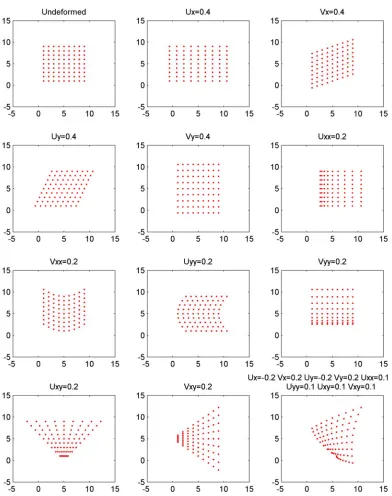
Figure 2–3. Deformations formulated by the 2nd-order shape function depending
on different shape parameters ... 24
Figure 3–1. Relationship between different types of errors, qualitative and
quantitative performances ... 38
Figure 3–2. Grey level histograms of different types of speckle patterns, from left
to right: airbrush, spray can, synthetic ... 39
Figure 3–3. Positive and negative camera distortions ... 41
Figure 3–4. The 3D calibration procedure, a spatial point P is projected onto the
XVIII
Figure 3–5. A region of interest is chosen from an experimental speckle image,
11×11 samples are uniformly selected and designed as the centres of
subsets with a size of 11×11 pixels ... 47
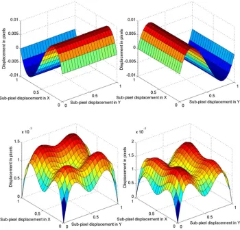
Figure 3–6. The distributions of mean errors and standard deviations of the
samples with respect to the 2D sub-pixel translations ... 48
Figure 3–7. Standard uncertainty estimation in an image-based measuring system
... 52
Figure 3–8. Estimation of deterministic errors by a black-box model ... 54
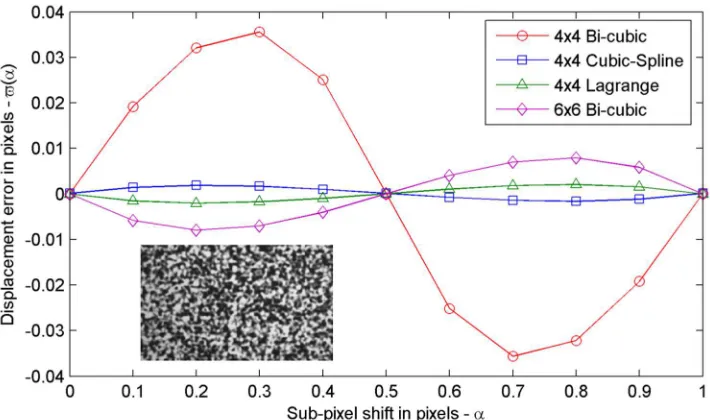
Figure 4–1. The anti-symmetric feature of sub-pixel registration bias due to
imperfect grey-intensity interpolation and additive Gaussian image
noise ... 77
Figure 4–2. Bias reduction method based on the anti-symmetric feature of
sub-pixel registration bias ... 80
Figure 4–3. The distribution of sample points shown in red crosses, subset size is
illustrated by a green square ... 81
Figure 4–4. The reduction of sub-pixel registration bias based on its
anti-symmetric feature, the x-axis denotes the sub-pixel increments while
the y-axis denotes the mean bias based on 1024 samples. ... 83
Figure 6–1. Dependency relationship of one inner point: (a) Q4-FE, (b) Cubic
Spline, (c) Kriging. ... 110
Figure 6–2. The self-adaptive control grid updating ... 119
Figure 6–3. A deformed image with a sinusoidal displacement field with a period
of 25 pixels ... 121
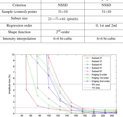
Figure 6–4. Amplitude loss vs period of the deformation sine wave for
XIX
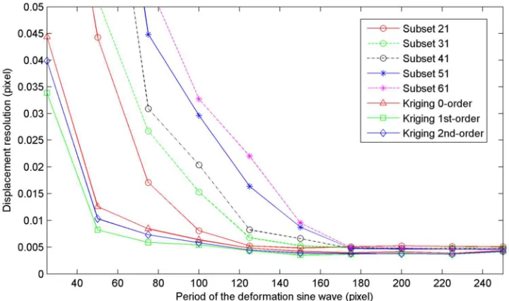
Figure 6–5. Displacement resolution vs period of the deformation sine wave for
subset-based DIC and Kriging-DIC ... 125
Figure 6–6. Displacement resolution vs spatial resolution under the criterion of
5% amplitude loss, a decrease in subset size and a increase in the
order of regression function are adopted respectively in the
subset-based DIC and Kriging DIC ... 125
Figure 6–7. Displacement resolution vs spatial resolution under the criterion of
1% amplitude loss, a decrease in subset size and a increase in the
order of regression function are adopted respectively in the
subset-based DIC and Kriging DIC ... 126
Figure 6–8. Reference and deformed grids shown as red and blue squares
respectively. ... 128
Figure 6–9. Calculated displacement fields in x-direction, from left to right:
Kriging DIC, Q4-FE DIC and Cubic Spline DIC. ... 128
Figure 6–10. Calculated displacement fields in y-direction, from left to right:
Kriging DIC, Q4-FE DIC and Cubic Spline DIC ... 129
Figure 6–11. The mesh grid of FE model (left plot) and the deformation under
tensile loading (right plot) ... 131
Figure 6–12. The interpolated FE displacement fields (in pixels) in x-direction (left)
and y-direction (right) ... 132
Figure 6–13. The selected region of interest from a real experimental image (DIC
Challenge 2D Dataset)... 132
Figure 6–14. The distribution of 78 chosen control points (Approach 1, 28 initial
points) on the reference image (left) and the deformed image (right).
XX
Figure 6–15. Evolution of GMSE: Approach 1 with 28 & 16 initial control points;
Approach 2 with 28 initial points. ... 133
Figure 6–16. Evolution of optimization parameters with increasing numbers of
control points. ... 134
Figure 6–17. Convergence of the objective function – Newton iteration... 136
Figure 6–18. The displacement errors in pixels (Approach 1, 28 initial points)
before Newton iteration (difference with the FE displacement fields)
in x-direction (left) and y-direction (right) ... 137
Figure 6–19. Displacement errors in pixels (Approach 1, 28 initial points) after
Newton iteration in x-direction (left) and y-direction (right) ... 137
Figure 6–20. The distribution of 78 chosen control points (Approach 1, 16 initial
points) on the reference image (left) and the deformed image (right)
... 138
Figure 6–21. The displacement errors in pixels (Approach 1, 16 initial points)
before Newton iteration (difference with the FE displacement fields)
in x-direction (left) and y-direction (right) ... 138
Figure 6–22. The displacement errors in pixels (Approach 1, 16 initial points) after
Newton iteration (difference with the FE displacement fields) in
x-direction (left) and y-x-direction (right) ... 139
Figure 6–23. Evolution of Kriging-DIC measurement error statistics ... 140
Figure 6–24. Trimmed speckle patterns, the reference image (left) and the
deformed image (right) ... 141
Figure 6–25. The distribution of 88 chosen control points (Approach 2, 28 initial
points) on the reference image (left) and the deformed image (right)
XXI
Figure 6–26. The displacement errors in pixels (Approach 2, 28 initial points)
before Newton iteration ... 142
Figure 6–27. Displacement errors in pixels (Approach 2, 28 initial points) after
Newton iteration in x-direction (left) and y-direction (right) ... 142
Figure 6–28. The experimental setup. ... 144
Figure 6–29. The distribution of initial control points and added control points
superimposed on the reference image. ... 145
Figure 6–30. Displacement fields (mm) calculated by Kriging DIC method in
x-direction (left) and y-x-direction (right). ... 145
Figure 6–31. Displacement fields (mm) calculated by the commercial system in the
x-direction (left) and y-direction (right) ... 145
Figure 6–32. The absolute difference between the displacement fields (mm)
calculated by Kriging DIC and the commercial system in the
x-direction (left) and y-x-direction (right). ... 146
Figure 7–1. Numerically generated speckles and the distribution of sample points
(red crosses) - 3 subsets are shown in green squares ... 161
Figure 7–2. Numerical case study 1: residual error comparison for a rigid-body
translation ... 163
Figure 7–3. Numerical case study 1: residual error comparison for an affine
deformation ... 163
Figure 7–4. Numerical case study 1: residual error comparison for Gaussian
image noise ... 163
Figure 7–5. Numerical case study 1: residual error comparison for the
combination of translation, affine deformation and Gaussian image
XXII
Figure 7–6. Numerical case study 2: calculated displacement fields, (a) by
subset-based DIC using Newton-Raphson scheme, (b) by Kriging regression
with local error estimate ... 165
Figure 7–7. Numerical case study 2: calculated strain fields, (a) by subset-based
DIC using 7×7 strain window, (b) by subset-based DIC using 15×15
strain window (c) by Kriging global method using 15×15 strain
window (d) by Kriging local method using 15×15 strain window. . 166
Figure 7–8. Experimental setup ... 167
Figure 7–9. Distribution of sample points (16×64) in the reference image of the
cantilever beam for Test 1 (a) and Test 2 (b) ... 168
Figure 7–10. Analytical displacement fields (mm): (a) x- and (b) y-directions
and strain distributions: (c) x-x and (d) y-y strains. ... 169
Figure 7–11. Diagonal elements of the optimized R matrix (16×64 centre nodes) in
(a) Test 1, (b) Test 2 ... 171
Figure 7–12. RMSE on the mean Kriging estimate of the displacement field
(y-direction): (a) Test 1; (b) Test 2... 173
Figure 7–13. Test 1 x-x strain field: (a) subset-based DIC using 21×21 strain
window; (b) Kriging global method using 21×21 strain window; (c)
Kriging local method using 21×21 strain window. (d) Kriging local
method using Kriging gradients ... 174
Figure 7–14. Test 2 x-x strain field: (a) subset-based DIC using 21×21 strain
window; (b) Kriging global method using 21×21 strain window; (c)
Kriging local method using 21×21 strain window. (d) Kriging local
XXIII
Figure 7–15. 3 local regions (A, B and C) are chosen on the beam in Test 2; a, b
and c are the points chosen from the same location of the 3 regions
... 175
Figure 7–16. Displacement STD shown in (a), (c) and (e) and Strain STD shown in
(b), (d) and (f), from top to bottom: Region A, B and C ... 176
Figure 7–17. The probability density for the strains and 95% confidence interval of
XXV
List of Tables
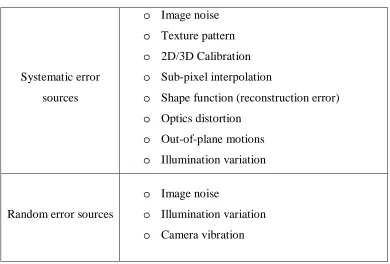
Table 3–1: DIC error sources ... 34
Table 3–2: DIC error classification ... 35
Table 4–1: Statistics of the numerical results in terms of standard deviation ... 84
Table 5–1: Correlation functions (only considering x- and y- directions)... 95
Table 6–1: Deformation parameters of the images ... 124
Table 6–2: Parameters of DIC algorithms ... 124
Table 6–3: Details of the 3 DIC methods ... 127
Table 6–4: Errors comparison (in pixels) ... 129
Table 6–5: Measurement error statistics (in pixels) ... 143
Table 6–6: Mean values and standard deviations of the absolute difference ... 146
Table 7–1: Optimized diagonal elements with global error estimate ... 169
Table 7–2: Concordance correlation coefficient based on Tchebichef shape
1 | P a g e
1
1
Introduction
In this chapter, the problem of DIC measurement error and uncertainty is considered
in terms of DIC algorithms, DIC error sources and DIC uncertainty estimation
methods. Then the characteristics of Kriging regression are introduced to highlight
the advantage of applying this technique for DIC error reduction and uncertainty
quantification. Finally, the outline and principal contributions of this thesis are
presented.
In the field of experimental mechanics, full-field measurement techniques have been
increasing in popularity during the past 30 years, for example, geometrical methods
such as Digital Image Correlation (DIC) and interferometric methods such as
holographic interferometry and speckle-pattern interferometry. Among these
methods, DIC technique has become the most popular full-field measurement
technique due to its simplicity in principle and implementation. The early
development of DIC can be traced back to the work by researchers at the University
2 | P a g e
optical-flow theory [5] which enables the tracking of speckle patterns and image
registration for quantitative measurements of the shape, displacement, and strain of
test objects. Nowadays, DIC has been extended and widely applied in many areas of
science and engineering thanks to the development of computer technology, digital
cameras and white-light optics.
Even though DIC is a widely used measurement method, the problem of
measurement error and uncertainty is still unsolved and needs further investigations.
In the following sections, it is briefly addressed in the consideration of DIC
algorithms, DIC measurement errors and DIC uncertainty estimation.
1.1 DIC algorithms
In general, DIC consists in maximising a correlation coefficient that is determined
by the grey-intensity difference between reference and deformed images, which
achieves a measurement of displacement field that is normally formulated by a
deformation mapping function known as shape function. Depending on the type of
shape function, DIC algorithms can be mainly classified into two categories [6]:
i. Local DIC algorithm: namely subset-based DIC [5], for which the shape
function is only applied within a subset in the Region of Interest (RoI). The
local approach is the most commonly used DIC algorithm with advantages of
simplicity [5], flexibility, suitability for parallel computation [7] and so on.
However, without inter-subset continuity, it is sensitive to grey-intensity
noise and may yield large uncertainties in measurement results [8]. Further,
its performance highly depends on the parameters input by the user, which
3 | P a g e ii. Global DIC algorithm [9-17]: known as full-field DIC, which applies the
shape function to the entire RoI and the displacement field is solved at once.
By imposing continuous constraints, the global approach is able to yield a
smooth displacement field with good sub-pixel accuracy. However, the
computational complexity can become significant when a large number of
Degrees of Freedom (DoF) is considered. The performance can degrade at
low spatial resolutions due to the smooth effect introduced by continuous
constraints. Moreover, the measurement accuracy still relies on the user’s
choice for parameters in most global DIC algorithms.
Thus, both the local and global DIC algorithms have advantages and disadvantages.
Generally for any DIC algorithm, a compromise has to be made between resolution
(precision) that indicates the capability of measuring a minimum change in the
measured quantity (e.g. displacement) and spatial resolution that represents the
capability of measuring at closely-spaced locations. An ideal DIC algorithm is
expected to be able to achieve an excellent resolution and an excellent spatial
resolution at the same time [18, 19].
1.2 DIC error sources
Though the DIC principle and experimental setup are relatively simple compared to
other techniques, DIC measurement results are not any less vulnerable to various
kinds of error sources in the measurement process, which inevitably contain a
certain level of uncertainty. Under ideal experimental conditions and using
state-of-the-art DIC algorithm, DIC measurement is reported as having an accuracy of a
hundredth of a pixel [20]. However, this kind of accuracy normally cannot be
4 | P a g e
for different DIC setups. The error sources can be generally classified into two
groups:
i. Experimental errors: The error sources occur in the image acquisition
process, normally related to experimental setups. The experimental error
sources consist of speckle-pattern quality [21-25], optical distortion [26-28]
and focus error [29], image acquisition noise [30-32] and so on, which are
fully contained in acquired digital images and will be propagated to final
measurement results through DIC algorithms.
ii. Algorithmic errors: The error sources are introduced in the process of
parameters measurement by applying DIC algorithms based on acquired
digital images. The algorithmic error sources include DIC correlation
criterion [20, 32-35], grey-intensity interpolation scheme [36, 37],
shape-function reconstruction error [38, 39] and so on. Algorithmic errors can be
significantly reduced by utilising a superior or more suitable DIC algorithm
with respect to a specific application.
In addition, DIC error sources can also be briefly classified into systematic errors
and random errors. Based on the investigation of DIC error sources, the works
related to DIC error analysis lead in two directions: one is to estimate measurement
uncertainty by quantifying the influence of error sources and the other is to increase
measurement accuracy by improving DIC algorithms or experimental setups. For
instance, local smoothing [32, 33, 40-42] techniques are normally applied in DIC
algorithms to reduce measurement errors due to various kinds of random error
sources. Generally these methods work effectively and are beneficial in terms of
simplicity of implementation. However, they probably can only achieve a local
5 | P a g e subject to the ad-hoc choice of parameterisation which results in inconvenience and
time-consuming problems in practical applications.
1.3 DIC uncertainty estimation
On the other hand, as a measuring technique, DIC should not be limited to obtaining
the measurement result but should also provide an estimate of measurement
uncertainty to show how good the result is, which is crucial for DIC applications and
still remains as an ongoing research topic. Because of intrinsic complexity of DIC
error sources [43], a reliable uncertainty quantification (UQ) of DIC results under
various experimental conditions is considered to be challenging. However, some
advances have already been made on UQ of DIC measurement in the recent years,
which can be briefly summarised as follows:
i. For systematic errors: For example, systematic error due to the use of
under-fitting shape function can be conveniently estimated by approximating
the shape function as a Savitzky-Golay low-pass filter based on the work of
Schreier et al. [39]. As presented in [44], the uncertainty of the
measurements (systematic and random errors) was predicted by using the
numerically generated deformed synthetic images, whereas the confidence
intervals of the identified material parameters were also simulated. A general
procedure to numerically simulate the unnotched Iosipescu test was proposed
in order to investigate the influence of DIC error factors such as spatial
resolution, noise and interpolation on the identification results with virtual
field method, Pierron et al. [45].
ii. For random errors: The measurement uncertainty caused by the most
6 | P a g e
photon noise) was analysed by several researchers using self-correlated
images with uncorrelated Gaussian intensity noise [5, 23, 46]. The results
demonstrate that the measurement uncertainty is proportional to the standard
deviation of image noise and inversely proportional to the average of the
squared grey level gradients and the subset size.
iii. Experimental analysis: Influence of hardware, acquisition system,
experimental condition and setup on DIC measurement uncertainty was
experimentally studied by using tensile loading tests [47], translation
experiments [48], the rigid-body-motion test [49] and so on.
iv. Theoretical analysis: Some efforts have also been made to theoretically
analyse DIC measurement uncertainty. For instance, a theoretical model was
derived by Pan et al [50] to indicate that the standard deviation error of
displacement measurement is closely related to the quality of speckle
patterns. Moreover, the effect of speckle size and density on the DIC
measurement uncertainty was also investigated based on numerical
experiments [21].
So far most studies that have been performed at DIC UQ consist in comparing DIC
measurement results with known displacements (e.g. using synthetic images) or
strains (e.g. obtained by strain gauges) and lead to very positive results [43], but
those results only apply to specific DIC setups. Concerning the quantification of
uncertainty due to various error sources under different DIC setups, a generic UQ
method should be developed to evaluate the reliability and accuracy of DIC
measurement results.
In an attempt to estimate measurement uncertainties in DIC in a general sense, an
7 | P a g e analytically based on the framework of subset-based DIC and the sum of squared
difference (SSD) DIC criterion [5, 23, 51]. Though this method is still restricted to
Gaussian image noise, a potential possibility is provided to extend the method to
handle uncertainty due to general DIC errors. In addition, there are also other
attempts of trying to achieve a generic expression for DIC UQ, for example, a
post-processing UQ method was proposed on the basis of the expected asymmetry of
correlation peak [35] in the correlation map of matched subsets. However, all the
above methods are derived from the subset-based DIC, which leads to a local
uncertainty estimate. On the contrary, it is more preferable to develop an UQ method
for DIC full-field measurement.
Inspired by existing approaches and related concerns, attempts were made to
introduce Kriging regression to DIC in order to effectively reduce DIC measurement
error and quantify the uncertainty for the full-field measurement.
1.4 Characteristics of Kriging regression
As widely used in the fields of spatial analysis and computer experiments [52, 53],
Kriging is a method that provides a best linear unbiased prediction (BLUP) for a RoI
based on observed values at design sites, which yields the most likely intermediate
values as opposed to the most ‘smooth’ intermediate values optimised by a
piecewise-polynomial spline. Moreover, if interpreted from a Bayesian framework
[53, 54], Kriging is modelled by a Gaussian process governed by a prior covariance
which straightforwardly provides the uncertainty estimate for predicted values. In
addition, thanks to the estimated uncertainty across the RoI, a self-adaptive infill
criterion can be employed to select new design locations required to achieve a
8 | P a g e
factors to the diagonal of Kriging correlation matrix [55, 56] enables the Kriging
regression method to regularise the measurement errors at the design sites which
further improves the accuracy of predicted values towards the ‘true’ values.
In light of potential applications in DIC for error reduction and uncertainty analysis,
the main features of Kriging regression technique can be summarised as follows:
i. Global: Kriging method aims to optimise full-field prediction model based
on observed data to achieve a best linear unbiased prediction, which is
different from most other DIC techniques that only consider the local
information or result in a local optimum.
ii. Flexible: Compared with shape functions used in other global DIC methods,
Kriging model is capable of adapting to an irregular distribution of control
points (as opposed to regular or uniform distributions) which provides the
flexibility for global DIC analysis.
iii. Automatic: Instead of using the ad-hoc choice of parameterisation in
classical DIC methods, the Kriging method can be used to achieve the
parameter values through a global optimisation algorithm which is
implemented automatically without user intervention. Furthermore, in the
proposed Kriging DIC method, the optimal number of control points is also
achieved automatically through a self-adaptive updating process.
iv. Consideration of errors: As aforementioned, measurement error of
observed data can be considered and incorporated into the Kriging regression
model, which significantly improves the accuracy of DIC results.
v. Uncertainty quantification: As a Gaussian process emulator, the Kriging
method is conveniently used to quantify the uncertainty of estimated
9 | P a g e obtained through a multivariate normal sampling process based on the
Kriging model.
1.5 Outline of the thesis
In the scope of applying the Kriging regression method to DIC for error reduction
and uncertainty analysis, two promising methods were carried out, they are, (1) a
new global DIC method named Kriging-DIC was developed by incorporating the
Kriging regression model into global DIC algorithm to formulate the displacement
field of the RoI as a global shape function with consideration of measurement error;
(2) a post-processing technique based on Kriging regression with error estimate (in
both global and local senses) was proposed to regularise the measurement error of
subset-based DIC (to improve measurement accuracy) and quantify the
measurement uncertainty of both displacement and strain results. The overall
structure of the thesis is presented in Figure 1–1.
Chapter 2: This chapter reviews DIC local and global algorithms to identify the
advantages and limitations of different kinds of DIC approaches. DIC objective
functions, solution strategies and displacement resolution and spatial resolution are
also considered.
Chapter 3: DIC errors and uncertainties are extensively reviewed. Concerning DIC
uncertainty analysis, the standard uncertainty analysis approach is briefly introduced.
Also a brief review of the Kriging regression method and Kriging-based uncertainty
analysis is provided.
Chapter 4: The significance of error reduction and uncertainty quantification in
10 | P a g e
derived based on the subset-based DIC algorithm (SSD criterion) by considering an
equivalent error variance due to common DIC error sources. Also the bias error in
DIC sub-pixel registration caused by Gaussian image noise under uniform
translation is estimated in the same framework. An error reduction method is
proposed in regard to the bias errors in DIC sub-pixel registration.
11 | P a g e
Chapter 5: Kriging regression theory is briefly addressed in this chapter. The
derivations of Kriging interpolation method are presented from both the framework
of best linear unbiased prediction (BLUP) and the framework of Bayesian inference.
Concerning measurement error of observed data, Kriging regression method is
presented by regularising measurement error from both global and local senses.
Furthermore, uncertainty analysis based on the Kriging regression method is also
addressed.
Chapter 6: In this chapter, a global (full-field) DIC algorithm with integrated
Kriging regression is proposed. Kriging regression model is employed as a full-field
shape function to formulate the displacement field of RoI. The displacement errors
of control points are quantified by introducing an error factor to the Kriging model.
In addition, a self-adaptive control grid updating strategy is developed on the basis
of the Mean Squared Error (MSE), which enables the proposed Kriging-DIC method
to achieve the optimal control grid automatically. Both numerical and experimental
case studies are used to verify the performance of Kriging-DIC method.
Chapter 7: The measurement uncertainty of subset-based DIC results is expressed
as a function of inverse Hessian matrix and SSD residual. The Kriging regression
method is developed as a post-processing technique including local error estimation,
which is able to improve the accuracy of measured subset-based DIC displacement
results and strain results. Uncertainty of the estimated displacement field is
illustrated in terms of the root mean square error (RMSE). Furthermore, strain
uncertainty is determined in terms of standard deviation (STD) by a multivariate
normal sampling process based on Kriging regression model. Both numerical and
12 | P a g e
Chapter 8: A review of key components of the research and main conclusions of
this thesis are presented. The important contributions of this study are highlighted
with suggestions for the future research which could be proceeded to extend current
investigations.
1.6 Contribution by the author
This thesis addresses the error reduction and uncertainty quantification problem in
Digital Image Correlation (DIC), which is crucial for DIC applications and remains
unsolved. The principal contribution of this thesis is introducing the Kriging
technique to DIC to deal with the measurement error and uncertainty from a new
perspective i.e. in the sense of a Gaussian-process. A new global DIC method
known as Kriging-DIC is developed to accurately measure the full-field
displacement in DIC. Further, a post-processing technique based on the Kriging
regression method with error estimation is also proposed to reduce the measurement
error and quantify the measurement uncertainty.
The author has summarised the above research findings into two journal papers on
Kriging-DIC method (J1) and Kriging-based DIC uncertainty quantification method
(J2) respectively. Also there are two conference papers presented at international
conferences. Paper C1 offers a good understanding of DIC error sources in the
testing of composite materials and Paper C2 covers the study of how to integrate the
estimated uncertainty of subset-based DIC into the Kriging regression model.
J1: D.Z. Wang, F.A. DiazDelaO, W.Z. Wang and J.E. Mottershead, ‘Full-field
digital image correlation with Kriging regression’. Optics and Lasers in Engineering,
13 | P a g e J2: D.Z. Wang, F.A. DiazDelaO, W.Z. Wang, X.S. Lin, E.A. Patterson and J.E.
Mottershead, ‘Uncertainty Quantification in DIC with Kriging Regression’. Optics
and Lasers in Engineering, doi: 10.1016/j.optlaseng.2015.09.006, In Press
C1: W.Z. Wang, D.Z. Wang, J.E. Mottershead and G. Lampeas, ‘Identification of
Composite Delamination Using the Krawtchouk Moment Descriptor’, Key
Engineering Materials, 569-570(2013) 33-40, doi:
10.4028/www.scientific.net-/KEM.569-570.33, (10th International Conference on Damage Assessment of
Structures (DAMAS 2013), July 8-10, 2013, Dublin, Ireland)
C2: D.Z. Wang, J.E. Mottershead, F.A. DiazDelaO and W.Z. Wang, ‘Kriging
Regression in Full-field Digital Image Correlation based on the Global and Local
Error Estimate’, the 16th International Conference on Experimental Mechanics, July
7-11, 2014, Cambridge, UK
15 | P a g e
2
2
Literature Review
Part 1 – DIC Algorithms
DIC local and global algorithms are reviewed in this chapter. It aims to identify the
advantages and disadvantages of these two types of DIC approaches. In addition,
DIC objective functions and solution strategies are briefly considered while a
discussion on DIC displacement resolution and spatial resolution is also presented.
Equation Chapter 2 Section 1
2.1 Objective functions
Digital Image Correlation is a full-field, non-contact measurement technique which
employs algorithms based on optical flow (which relates to the classic
Lucas-Kanade tracker) to determine underlying deformation between images [57]. Since it
is normally impossible to match individual pixels in different images, the area match
16 | P a g e
the pixels within the area. The Region of Interest (RoI) in the image may be divided
into a large number of small areas so called ‘subsets’ normally with overlapping
[18]. On the other hand, the whole RoI could also be treated as a large ‘subset’ for
analysis. On that basis, algorithms in DIC could be categorized as either local
methods (subset-based) or global methods.
The matching criterion is normally interpreted in two forms, they are, minimization
of Sum of Squared Differences (SSD) [58] of grey intensities between an image pair
and maximization of Cross-correlation Coefficient (CC) [58] between two images.
Assuming intensity functions are continuous for the reason of simplicity, these two
criteria can be written as:
( )
(
)
( )
(
)
( )
(
)
( )
(
)
2
arg min ( , ), , , d
arg max ( , ), , , d
g x u x y y v x y f x y g x u x y y v x y f x y
Θ
Θ
= + + − Θ
= + + × Θ
∫
∫
SSD
CC C
C
(2-1)
where Θ denotes the RoI in the first image. The displacement
(
u x y v x y( , ),( )
,)
may also be understood as the optical flow of the speckle-pattern intensity from areference image f x y( , ) to its corresponding deformed image g x y( , ) . It is
noteworthy that there are also other types of DIC criteria applied including Sum of
Absolute Difference (SAD) [59], Parametric Sum of Squared Difference (PSSD) [60]
with additional unknown parameters and extended SSD and CC criteria [33, 61] e.g.
Normalized Sum of Squared Differences (NSSD), Normalized Cross-correlation
Coefficient (NCC), Zero-Normalized Sum of Squared Differences (ZNSSD) and
Zero-Normalized Cross-Correlation Coefficient (ZNCC). Though the mathematical
expressions of the correlation criteria are different, original and extended CC criteria
17 | P a g e
2.2 Solution strategies
In order to find a solution for the DIC correlation criterion, the displacement field of
a subset or RoI should be formulated by a shape function with finite unknown
parameters to be determined. These parameters act as Degrees of Freedom (DoF)
and are used to allow images to distort. Generally the DIC solution is related to the
framework of ill-posed inverse problems [62]. For both global and local DIC
approaches, the displacement field
(
u x y v x y( , ), ( , ))
can be approximated as a linear combination of chosen basis functions of unknown parameters [8, 18, 63] with finitedimension n, expressed as
1
1
( , ) ( , )
( , ) ( , )
j
j
n
j u
j
n
j v
j
u x y x y p v x y x y p
µ
µ
=
=
≈
≈
∑
∑
(2-2)
where µj( , );x y j=1, 2,…,n are kernel functions and puj,pvj;j=1, 2,…,n are combination coefficients. Since g x u x y y
(
+ ( , ), +v x y( , ))
is an implicit function of(
u x y v x y( , ), ( , ))
, an iterative process is usually applied to solve the minimisation problem in Equation (2-1) (SSD criterion). Different types of algorithms e.g. geneticalgorithms [64-66], Levenberg–Marquardt algorithm [17, 39], Newton–Raphson
iteration [2, 36, 67-69], and multi-grid solver [10] may be used to solve the
minimization problem. However among the above algorithms, a detailed
examination [70] has shown that the spatial-domain Newton-Raphson algorithm
provides the highest accuracy and the implementation of the NR algorithm is
18 | P a g e
Therefore, an approximate solution of the full-field displacement,
(
u x y v x y( , ), ( , ))
, may be obtained by the NR iteration [10, 11, 71, 72]: (considered as the governingequation in ith iteration)
(
1)
i i+ − i = i
M p p b (2-3)
where
1 1 2 2
T
n n
i i i i i i i
u v u v u v
p p p p p p
=
p ⋯ is a 2n×1 vector, i
M are 2n×2n matrices and bi are 2n×1 vectors, with components given by
( )
Mjk i ij ikdΘ
= Ξ ×Ξ Θ
∫
(2-4)and
( )
bj i ij(
f x y( , ) g x u y v( i, i) d)
Θ
= Ξ ×
∫
− + + Θ (2-5)where T 1 1 2 ( , ) ( , ) ( , ) ( , ) i i i i i i i n i i n n
g x u y v x g x u y v
y g x u y v
x g x u y v
y µ µ µ µ ∂ + + ∂ ∂ + + ∂ = ∂ + + ∂ ∂ + + ∂
Ξ ⋮ and ,j k=1, 2,…, 2n (2-6)
The gradients ( , )
i i
g x u y v
x
∂ + +
∂ and
( i, i)
g x u y v y
∂ + +
∂ in equations (2-4) and (2-5)
are in principle updated at each iteration. However, as proposed by Sutton [57, 73],
the grey-level gradients may be calculated from the reference image rather than the
19 | P a g e Since the sub-pixel accuracy is normally required for DIC measurement, the
objective function (correlation criterion) should be evaluated at non-integer locations.
Therefore, an interpolation method has to be employed to approximate the grey
values among pixels. A comprehensive catalogue of interpolation methods used in
the field of image processing was presented [37], which also provides a general
comparison and valuable comments for different interpolation approaches. The
interpolation bias was studied through the analytical phase error of interpolation
filters [36] and experimental validation [74] while high-number-tap interpolation
filters were recommended for related applications in DIC [57]. Aiming to enhance
the accuracy of B-spline interpolation used in DIC, a technique was proposed by
employing a family of recursive interpolation schemes and its inverse gradient
weighting form [75].
Besides spatial-domain iterative methods (like Newton iteration), there are also
some other strategies which have been employed in order to achieve the
displacement field with sub-pixel accuracy [20], including correlation coefficient
curve-fitting [76, 77] or interpolation methods [78, 79] (so-called peak finding
algorithms [29]), gradient-based methods [80-83], artificial neural network methods
[84, 85] and so on. However, these methods can hardly be used to achieve more
accurate measurement than the NR iteration method and are normally subject to the
intrinsic lack of deformational DoF of the subset, namely the application of shape
functions [29].
2.3 Displacement resolution and spatial resolution
The displacement resolution is defined as the smallest change of the displacement
20 | P a g e
86]. In practice, it is quantified by the noise level of the measured displacement in
terms of standard deviation and depends on various error sources and on the
sampling resolution of the imaging system. In contrast to the displacement
resolution, the spatial resolution is defined as the smallest distance between two
independent data points [18, 86]. In practice, a more reasonable definition for the
spatial resolution is one-half of the period of the highest frequency component
contained in the frequency band of the displacement data [87]. The spatial resolution
of subset-based DIC can be approximately considered as the subset size while the
spatial resolution of global DIC depends on the number of measurements obtained
within the RoI. It is desirable to have small values for both the displacement
resolution and the spatial resolution, which indicates a more favourable
measurement [19]. Fundamentally a compromise is generally made between the
displacement and spatial resolutions for a DIC algorithm [57]. In [19], the spatial
resolution was re-defined for both local and global DIC algorithms and evaluated
with the help of deformed images with a unidirectional in-plane sinusoidal
deformation field, which enables a fair comparison between different DIC
algorithms by plotting displacement resolution versus spatial resolution in the same
figure.
2.4 Local vs global DIC algorithms
There are the different ways applying DIC algorithms to the RoI, which belong to
two general classes: local (subset-based) methods and global (full-field) methods,
both of which have been well developed. The local approach is perhaps the better
established of the two because of its simplicity [5], flexibility, and suitability to
21 | P a g e local method being more sensitive to measurement noise than the global approach
and yields relatively larger uncertainties in the measured displacement [8].
Consequently, measured displacement field of the local method is unsmooth with
discontinuities, for example, as shown in Figure 2–1. Thus a smoothing technique is
normally applied as a post-processing operation especially for calculating strain
results [88].
Figure 2–1. Discontinuities in the measured displacement field from a test of
composite material based on a commercial DIC system (Dantec Q400)
Alternatively, the global approach imposes continuous constraints and treats the RoI
as a whole, thereby enabling smooth displacement fields to be achieved together
with good sub-pixel accuracy. However, there are also challenges for global method.
Firstly, apart from the limited number of DoF involved in the local methods, the
number of DoF that needs to be solved simultaneously increases quickly in global
methods as the spatial resolution decreases. The associated computational
complexity becomes significant [8, 72], which may result in failure to solve the
inverse of the Hessian matrix during NR iteration. Secondly, the continuous
constraint of global methods can become a disadvantage by degrading the spatial
-20 -15 -10 -5 0 5 10 15
-25
-20
-15
-10
-5
0
5
10
15
20
25 -0.15
22 | P a g e
resolution when localized phenomena occur (e.g. cracks, sliding and shear-bands)
since discontinuities may be smoothed out or lead to non-convergence of the
optimisation [10, 89].
2.5 Local DIC algorithms
By meshing the RoI with a set of evenly spaced grid points in the reference image, a
local method may be applied on each of the subsets with the centres located at the
grid points in order to find matched subsets in the deformed image as shown in
Figure 2–2. According to the objective function shown in Equation (2-1), unknown
parameters for each subset are solved by the aforementioned NR iteration. Normally
the displacement field of one subset is formulated by a shape function (up to a
second-order) around the centre point. For instance, a second-order Taylor
expansion around the centre node at ( ,x y0 0) is applied for the coordinate transformation as:
2 2
1 1
0 2 2
2 2
1 1
0 2 2
( , ) u
( , )
i j x y xx yy x y
i j x y xx yy x y
u x y u x u y u x u y u x y v x y v v x v y v x v y v x y
= + ∆ + ∆ + ∆ + ∆ + ∆ ∆
= + ∆ + ∆ + ∆ + ∆ + ∆ ∆ (2-7)
where ∆ = −x xi x0 and ∆ =y yj−y0 . u v0, 0 are the x- and y-directional
displacement components of the centre node at ( ,x y0 0) , u v ux, x, y,vy are the components of the first-order displacement gradient and uxx,vxx,uyy,vyy,uxy,vxy are
the components of the second-order displacement gradient. Meanwhile, some of the
typical deformations described by a second-order shape function are demonstrated in
Figure 2–3. In general, the subsets are artificially designated as squares in the
23 | P a g e Gaussian weighted windows [90, 91] are also successfully applied in order to
achieve an optimal compromise between the systematic errors and random errors.
Under the assumption of only pure translations existing in sufficiently small subset
regions, displacement field could be approximated by a zero-order shape function
which only contains the first term in Equation (2-7). This approximation was
developed and applied in both physical space [4, 92] and Fourier space [76, 93] in
the 1980s and 90s. Based on the requirement of detecting a complex spatial
deformation, the first- and second-order shape functions [2, 94] are employed in
local methods with a higher computational cost. Furthermore, a simplified form of
Hessian matrix is also derived by ignoring the second-order partial derivatives
without loss of accuracy [67, 94]. The initial values used to start the NR iteration
can be calculated based on a fast cross-correlation technique using the zero-order
shape function [67, 94].
Figure 2–2. The illustration of subset-based DIC method (without overlapping
subsets), the uniformly distributed square subsets (centre nodes marked in ‘+’) are
initialized in the reference image (left) while the matched deformed subsets (centre
24 | P a g e
Figure 2–3. Deformations formulated by the 2nd-order shape function depending on
different shape parameters
In addition, a so-called analytic propagation function was developed to produce
accurate initialization for the NR iteration [95]. A method used with the multiple
growing cracks is implemented by modifying the local method to allow the crack
25 | P a g e improved local method was proposed in order to tackle discontinuities of the
displacement field through splitting the subset into two sections where each of the
sections is matched using independent deformation parameters [97]. On account of
the possible error propagation of the general subset-based DIC method, a
reliability-guided technique [98-101] was developed to optimise the calculation path of subsets
to enhance the robustness in discontinuous and large-deformation areas.
2.6 Global DIC algorithms
Instead of calculating the displacement field of RoI based on a large number of
independent subsets, a global framework was proposed to solve the minimization
problem at once for the whole RoI. In the global approach, displacement field is
formulated by a sophisticated shape function with a large number of DoF which is
able to capture detailed deformation. The iteration process as shown in Equation
(2-3) is essentially the same as in the local methods but works over the whole RoI.
Various different types of full-field shape functions were studied. The full-field DIC
methods are summarized in the following sections:
2.6.1 FE based DIC
Due to extensive DIC applications in experimental mechanics, Finite Element (FE)
shape functions naturally became a popular choice to formulate the displacement
field, which satisfies the requirement of displacement continuity among elements.
For example, the bilinear rectangular elements (Q4-FE) introduced in [9-11] are
used to mesh the RoI globally. The basic idea is shown as follows: ( , )x y represents
26 | P a g e
displacements of all the nodes on the meshed grid in the RoI. In order to assemble
all the subsets together for a global analysis, e
G is employed as the nodal assembly
matrix [9, 102] for the aforementioned element. Thus the displacements of the point
( , )x y in terms of the Q4-FE [102] shape function are described as:
4 1 4 1 ( , ) ( , ) and ( , ) ( , ) j j e j u
j e e
e
j v
j
u x y x y p v x y x y p
= = = Φ = = Φ
∑
∑
p G p (2-8)
where Φj( , );x y j =1, 2,…, 4 are the Q4-FE kernel functions. A new solution
strategy known as the non-linear multi-grid solver [10] is integrated into the Newton
iterative procedure to efficiently find the global minima of the correlation criteria.
Apart from the Q4-FE elements, linear triangular (T3-FE) [103], higher-order FE
shape functions like beam elements [104] and planar iso-parametric elements (with
24 DoF) [105] are also used through the same framework. Based on standard FE
basis functions, a new method called PGD-DIC [72] employs a proper generalized
decomposition technique to transform the 2D or 3D DIC problem into two 1D
problem only involving 1D mesh. This method is able to significantly reduce the
computational cost of traditional FE-DIC but is subject to separability of the
displacement fields. On account of the connections between FE-DIC and the
mechanical properties identification using FE Model Updating (FEMU), the nodal
displacements measured by FE-DIC are easily integrated into the FEMU framework
[106]. Furthermore, the introduction of parallel computation and the incorporation of
a mixed optical/mechanical cost function [107] further improve the application of
27 | P a g e
2.6.2 Extended FE-DIC
In the presence of discontinuities like cracks and shear bands, the aforementioned
FE-DIC methods may become inappropriate for the application. A feasible approach
is implemented to exclude the discontinuities from the RoI by using refined meshes
in the vicinity [13]. However, the refined meshes are normally unfavourable on
account of the accuracy and computational cost. In contrast to mesh refinements,
eXtended FE method (XFEM) [10, 12] was introduced to the FE-DIC to add extra
DoF with enriched elements and allow to measure irregular displacements due to
various kinds of discontinuities [89]. Also a strategy of optimising the crack path
configuration was proposed in [89]. An extended correlation technique by
introducing discontinuous enrichment to FE shape functions was also proposed to
allow the partition of FE elements when detecting shear-band like discontinuities
[10]. Furthermore, an additional penalization is incorporated into the extended
FE-DIC [108] to reduce measurement uncertainty, estimate crack tip locations and
evaluate stress intensity factors [109].
2.6.3 P-DIC
In order to reduce the dependency of DIC measurement results on the user’s choice
of parameters and accurately measure high heterogeneous deformations, a new
global DIC algorithm with a self-adaptive higher-order mesh was proposed based on
p-adaptive finite element analysis [110], known as p-DIC [19]. When a p-adaptive
mesh was used, degrees of freedom of the elements in the mesh could be adjusted to
sufficiently represent the real deformation field. The mesh refinement was carried
out according to a posterior residual error estimation based on an approach using
multiple passes algorithms [111]. In contrast to the shape functions used in