This is a repository copy of Structured total least norm and approximate GCDs of inexact polynomials .
White Rose Research Online URL for this paper: http://eprints.whiterose.ac.uk/3768/
Article:
Winkler, J.R. and Allan, J.D. (2008) Structured total least norm and approximate GCDs of inexact polynomials. Journal of Computational and Applied Mathematics, 215 (1). pp. 1-13. ISSN 0377-0427
https://doi.org/10.1016/j.cam.2007.03.018
Reuse
Unless indicated otherwise, fulltext items are protected by copyright with all rights reserved. The copyright exception in section 29 of the Copyright, Designs and Patents Act 1988 allows the making of a single copy solely for the purpose of non-commercial research or private study within the limits of fair dealing. The publisher or other rights-holder may allow further reproduction and re-use of this version - refer to the White Rose Research Online record for this item. Where records identify the publisher as the copyright holder, users can verify any specific terms of use on the publisher’s website.
Takedown
If you consider content in White Rose Research Online to be in breach of UK law, please notify us by
promoting access to White Rose research papers
White Rose Research Online
Universities of Leeds, Sheffield and York
http://eprints.whiterose.ac.uk/
This is an author produced version of a paper published in Journal of
Computational and Applied Mathematics.
White Rose Research Online URL for this paper: http://eprints.whiterose.ac.uk/3768/
Published paper
Winkler, J.R. and Allan, J.D. (2008) Structured total least norm and
approximate GCDs of inexact polynomials, Journal of Computational and
Structured total least norm and approximate
GCDs of inexact polynomials
Joab R. Winkler,
aJohn D. Allan
aaDepartment of Computer Science, The University of Sheffield, Regent Court,
211 Portobello Street, Sheffield S1 4DP, United Kingdom
[email protected], [email protected]
Abstract
The determination of an approximate greatest common divisor (GCD) of two in-exact polynomials f =f(y) and g =g(y) arises in several applications, including signal processing and control. This approximate GCD can be obtained by comput-ing a structured low rank approximationS∗(f, g) of the Sylvester resultant matrix
S(f, g). In this paper, the method of structured total least norm (STLN) is used to compute a low rank approximation ofS(f, g), and it is shown that important issues that have a considerable effect on the approximate GCD have not been considered. For example, the established works only yield one matrix S∗(f, g), and therefore one approximate GCD, but it is shown in this paper that a family of structured low rank approximations can be computed, each member of which yields a different ap-proximate GCD. Examples that illustrate the importance of these and other issues are presented.
Key words: Sylvester matrix, structured total least norm, approximate greatest common divisor
1 Introduction
f(y) =
m X
i=0
aiym−i and g(y) = n X
j=0
bjyn−j, (1)
are coprime, and the maximum normwise error in their coefficients ise, then a minor structured perturbation of the coefficients to ai +δai and bj +δbj,
where δa={δai} m
i=0 and δb={δbj}
n
j=0, and
kδak ≤e≪ kak, kδbk ≤e ≪ kbk, k·k=k·k2, (2)
may cause the perturbed inexact polynomials
˜
f(y) =
m X
i=0
(ai+δai)ym−i and ˜g(y) = n X
j=0
(bj+δbj)yn−j, (3)
to have a non-constant GCD. Even if it is required to compute the smallest perturbations δai and δbj such that the polynomials (3) have a non-constant
GCD, different noisy realisations f(y) and g(y) of their theoretically exact forms yield different approximate GCDs, all of which are valid if (2) is satisfied.
The computation of an approximate GCD of the inexact polynomials (1) has been considered by several authors. For example, Corless et. al. [5], and Zarowski et. al.[13], use theQR decomposition of the Sylvester resultant ma-trixS(f, g) [3], which will henceforth be called the Sylvester matrix. Similarly, the singular value decomposition of S(f, g) is used in [4] in order to compute an approximate GCD, but both these decompositions do not preserve its struc-ture. In particular, the smallest non-zero singular value ofS(f, g) is a measure of its distance to singularity, but this is the distance to an arbitrary rank deficient matrix, and not the distance to the nearest rank deficient Sylvester matrix. Karmarkar and Lakshman [8] use optimisation techniques in order to compute the smallest perturbations that must be applied to the coefficients of two polynomials such that they have a non-constant GCD, and Pan [11] uses Pad´e approximations to compute an approximate GCD. Zeng [14] uses partial singular value decompositions of Sylvester subresultant matrices, and an iterative algorithm is then used to calculate the factors of the GCD.
In this paper, the perturbationsδai, i= 0, . . . , m, andδbj, j = 0, . . . , n,in (3)
• Since the GCD off(y) and g(y) is equal to, up to an arbitrary scalar mul-tiplier, the GCD of f(y) and αg(y) where α is an arbitrary non-zero con-stant, it follows that the Sylvester resultant matrixS(f, αg) should be used when it is desired to compute an approximate GCD off(y) andg(y). Since
S(f, αg) 6= αS(f, g), the inclusion of α permits a family of approximate GCDs, rather than only one approximate GCD, to be computed. In par-ticular, it is shown in the examples in Section 4 that the restriction α = 1 yields unsatisfactory solutions, but that the inclusion of α allows signifi-cantly improved solutions to be obtained.
• The method of STLN yields a non-linear least squares problem with an equality constraint, and the minimisation of the residual leads to a non-linear algebraic equation that is solved iteratively. It is shown that a stop-ping criterion that is based on a small normalised residual may lead to a poor or incorrect solution, and that an additional stopping criterion that is based on the singular values of S( ˜f ,˜g) must be included.
• The perturbed inexact polynomials ˜f(y) and ˜g(y) are obtained by comput-ing the perturbations δai, i = 0, . . . , m, and δbj, j = 0, . . . , n, and a
com-puted approximate GCD is valid if (2) is satisfied. This condition requires that the norm of these perturbations be less than the maximum permissible normwise error in the coefficients because it guarantees that the perturbed inexact polynomials ˜f(y) and ˜g(y) are legitimate realisations of the theoret-ically exact forms off(y) andg(y), respectively. This criterion has not been considered in previous work as a condition for the acceptance or rejection of an approximate GCD.
It is important to note that if interest is restricted to the computation of a structured low rank approximation of S(f, g) and an approximate GCD com-putation is not required, then the default value α = 1 must be used. In this paper, however, it is desired to compute a family of approximate GCDs from structured low rank approximations ofS(f, αg), and thus the introduction of
αis required. Different values ofαyield different structured low rank approxi-mations, and each of these approximations is a candidate for the computation of an approximate GCD of f(y) and g(y). It will be shown, however, that it is not possible to construct an approximate GCD for all values ofαbecause a necessary equality constraint is not satisfied exactly, and the numerical rank of S( ˜f ,g˜) is not defined, for all values α.
2 The Sylvester matrix
The Sylvester matrix S(f, αg)∈R(m+n)×(m+n) is equal to
S(f, αg) =
a0
a1 a0
... a1 . ..
am−1 ... ... a0
am am−1 . .. a1
am . .. ...
. .. am−1
am αb0
αb1 αb0
... αb1 . ..
αbn−1 ... ... αb0
αbn αbn−1 . .. αb1
αbn . .. ...
. .. αbn−1
αbn ,
where the coefficientsai off(y) occupy the firstncolumns, and the coefficients
αbi of αg(y) occupy the last m columns. It is shown in [3] that if the degree
of the GCD off(y) and αg(y) is equal tod, then the rank of S(f, αg) is equal to (m+n−d), that is, the rank loss of the Sylvester matrix is equal to the degree of the GCD of f(y) andαg(y). The condition number of S(f, αg) is a function of α, and it therefore follows that the accuracy and stability of the numerical computation of the GCD off(y) andαg(y) is dependent onα. This will be confirmed in Section 4, where several examples are considered, and it will be shown that an incorrect value ofα leads to poor results.
The k’th Sylvester matrix, or subresultant, Sk ∈ R(m+n−k+1)×(m+n−2k+2) is
a submatrix of S(f, αg) that is formed by deleting the last (k −1) rows of
S(f, αg), the last (k−1) columns of the coefficients off(y), and the last (k−1) columns of the coefficients ofαg(y).
Example 2.1
S1 =S(f, αg) =
a0 αb0
a1 a0 αb1 αb0
a2 a1 a0 αb2 αb1 αb0
a3 a2 a1 αb3 αb2 αb1 αb0
a4 a3 a2 αb3 αb2 αb1
a4 a3 αb3 αb2
a4 αb3
,
S2 =
a0 αb0
a1 a0 αb1 αb0
a2 a1 αb2 αb1 αb0
a3 a2 αb3 αb2 αb1
a4 a3 αb3 αb2
a4 αb3
, S3 =
a0 αb0
a1 αb1 αb0
a2 αb2 αb1
a3 αb3 αb2
a4 αb3
. 2
Each matrix Sk is partitioned into a vector ck ∈ Rm+n−k+1 and a matrix
Ak =Ak(α)∈R(m+n−k+1)×(m+n−2k+1), where ck is the first column of Sk, and
Ak is the matrix formed from the remaining columns of Sk,
Sk= ck Ak = ck
coeffs. of f(y)
coeffs. of αg(y)
.
The application of the method of STLN to the computation of an approximate GCD of the inexact polynomialsf(y) and αg(y) requires that the equation
Akx=ck, x∈Rm+n−2k+1, (4)
be considered. The following theorem is established in [7,9,15].
Theorem 2.1 Consider the polynomialsf(y)andαg(y), where f(y)andg(y)
are defined in (1), and let k be a positive integer, where 1≤ k ≤ min (m, n). Then
(1) The dimension of the null space of Sk is greater than or equal to one if
(2) A necessary and sufficient condition for the polynomials f(y) and αg(y)
to have a common divisor of degree greater than or equal to k is that the rank of Sk is less than or equal to (m+n−2k+ 1).
It is recalled that f(y) and αg(y) are inexact and coprime, and that their theoretically exact forms have a non-constant GCD. There therefore exist perturbations δf(y) and αδg(y) such that f(y) +δf(y) and α(g(y) +δg(y)) have a non-constant common divisor, that is, if hk ∈ Rm+n−k+1 and Ek ∈
R(m+n−k+1)×(m+n−2k+1) are structured perturbations ofckand Akrespectively,
it follows from Theorem 2.1 that the equation
(Ak+Ek)x=ck+hk, (5)
which is the perturbed form of (4), has an exact solution.
It follows from Theorem 2.1 that (5) has a solution if and only iff(y) +δf(y) and g(y) +δg(y) have a common divisor of degree greater than or equal to k. The computation of a structured low rank approximation ofS(f, αg) therefore requires the determination of a structured matrix Ek and a structured vector
hksuch that (5) possesses a solution for whichAkandEkhave the same
struc-ture, andck and hk have the same structure. This is an overdetermined
equa-tion, andk is initially set equal to its maximum value,k =k0 = min (m, n). If
a solution exists, then the degree of the GCD off(y) +δf(y) andg(y) +δg(y) is equal to k0. If this equation does not possess a solution, then k is reduced
to k0−1, and if a solution exists for this value of k, then the degree of the
GCD of f(y) +δf(y) and g(y) +δg(y) is equal to k0 −1. If a solution does
not exist, then k is reduced to k0 −2, and this process is repeated until (5)
possesses a solution. This result is used in the next section in order to compute a structured low rank approximation of S(f, αg).
3 The method of STLN for a Sylvester matrix
It is shown in this section that the method of structured total least norm (STLN) can be used to compute a solution of (5), subject to the constraints onEk and hk that are stated in the previous paragraph.
Letz ={zi}im=0+n+1 be the vector of perturbations of the coefficients off(y) and
αg(y) such that their perturbed forms have a non-constant common divisor. In particular, let zi be the perturbation of the coefficient ai, i = 0, . . . , m, of
f(y), and let zm+1+j be the perturbation of the coefficient αbj, j = 0, . . . , n,
Bk:= hk Ek =
z0 zm+1
z1 z0 zm+2
... z1 . .. ... . ..
zm−1 ... . .. z0 zm+n . .. zm+1
zm zm−1 . .. z1 zm+n+1 . .. zm+2
zm . .. ... . .. ...
. .. zm−1 . .. zm+n
zm zm+n+1
,
where hk is equal to the first column ofBk, and Ek is equal to the last (m+
n−2k+ 1) columns ofBk.
Equation (5), which is non-linear, is solved iteratively for the perturbations
zi, i= 0, . . . , m+n+ 1, such that the structures of Ek and hk are retained. In
particular, the residualr(z, x) that is associated with an approximate solution of (5) due to the approximate perturbationshk and Ek is
r(z, x) =ck+hk−(Ak+Ek)x, hk =Pkz, Ek =Ek(z), (6)
and it is required to minimisekDzksubject to the constraint r(z, x) = 0. The matrixD∈R(m+n+2)×(m+n+2) is diagonal and accounts for the repetition of the
elements of z in Bk. In particular, each of the perturbations zi, i = 0, . . . , m,
occurs (n−k + 1) times in Bk, and each of the perturbations zi, i = m+
1, . . . , m+n+ 1, occurs (m−k+ 1) times inBk, and thus
D=
D1 0
0 D2
=
(n−k+ 1)Im+1 0
0 (m−k+ 1)In+1
.
It is shown in [7,9,15] if r(z, x) is linearised and the 2-norm is used, this constrained minimisation leads to a least squares problem with an equality constraint (the LSE problem),
min δz D 0 δz δx
−(−Dz)
subject to C
δz δx
=q, (7)
where k·k=k·k2, C ∈R(m+n−k+1)×(2m+2n−2k+3) is a function of A
and q ∈ Rm+n−k+1 is a function of the residual of (6) due to an approximate solution of this equation.
If E ∈ R(m+n+2)×(2m+2n−2k+3), ω ∈ R2m+2n−2k+3 and p ∈ Rm+n+2 are defined as
E =
D1 0 0
0 D2 0
, ω=
δz
δx
and p=−Dz,
respectively, where δz∈Rm+n+2 and δx∈Rm+n−2k+1, then the LSE problem (7) can be written as
min
w kEω−pk subject to Cω =q.
Algorithm 3.1 implements the LSE problem using the QR decomposition [6], and the initial value ofxin this iterative algorithm is given by settingr(z, x) =
hk =Ek = 0 in (6),
x= arg min
t kAkt−ckk. (8)
3.1 Solution methods for the LSE problem
The LSE problem (7) is usually solved by the method of weights [1,2,10]. Al-though this method transforms the LSE problem into an unconstrained least squares problem that can be solved by standard methods, it is necessary to introduce a weight parameter τ whose value is specified by heuristic methods. Van Loan [10] recommends that τ = µ−1
2, but Barlow [1], and Barlow and
Vemulapati [2], recommend that τ =µ−1
3, where µ is the machine precision.
The heuristic nature of τ is a disadvantage of this method because the con-vergence of the algorithm for the method of weights is critically dependent on the value ofτ. In particular, if τ is too large or too small, the algorithm may converge slowly, or it may converge to an inaccurate solution, or it may not converge at all [1]. Furthermore, it is noted in [1] that the algorithm for the method of weights converges quickly for all but ill-conditioned problems. The
Algorithm 3.1: STLN for a Sylvester matrix
Input The polynomials f(y) and g(y), the scalar α, a value for k, where 1≤k ≤min (m, n), and the tolerances ǫx and ǫz.
Output Polynomials ˜f(y) =f(y) +δf(y) and ˜g(y) = g(y) +δg(y) such that the degree of the GCD of ˜f(y) and ˜g(y) is greater than or equal to k.
Begin
(1) Form thek’th Sylvester matrix Sk from f(y), g(y) and α.
(2) Set Ek = 0 and hk = 0, and compute the initial value of x from (8).
Construct the residualr(z, x) =ck−Akx, the matrix Yk fromx, and the
matrix Pk.
(3) Repeat
(a) Compute the QR decomposition of CT,
CT =QR=Q
R1
0
.
(b) Set w1 =R−1Tq.
(c) Partition EQ as
EQ=
E1 E2
,
whereE1 ∈R(m+n+2)×(m+n−k+1) and E2 ∈R(m+n+2)×(m+n−k+2).
(d) Compute
z1 =E2†(p−E1w1).
(e) Compute the solution
y=Q
w1
z1
.
(f) Set x:=x+δx and z :=z+δz.
(g) Update Ek and hk from z, and Yk from x. Compute the residual
r(z, x) = (ck+hk)−(Ak+Ek)x.
Until kkδxxkk ≤ǫx AND kkδzzkk ≤ǫz.
4 Examples
This section contains several examples that illustrate the method of STLN for the computation of a structured low rank approximation ofS(f, αg) when it is required to compute an approximate GCD of f(y) and g(y) from this low rank approximation. It is shown that Algorithm 3.1 does not always yield a valid solution, and refinements to it are therefore required. Polynomials of high degree with roots of high multiplicity are considered in the examples in order to establish the robustness of the proposed algorithm.
The given inexact polynomials f(y) and g(y) are constructed by perturbing their theoretically exact forms ˆf = ˆf(y) and ˆg = ˆg(y). In particular, let
µ= 1/ε be the signal-to-noise ratio,
δfˆ
=ε
fˆ
and kδˆgk=εkgˆk,
where the norm of a polynomial is equal to the 2-norm of its coefficients. If
cf ∈ Rm+1 and cg ∈ Rn+1 are vectors of random variables, all of which are
uniformly distributed in the interval [−1, . . . ,+1], then the perturbations δfˆ
and δˆg are given by
δfˆ=ε
fˆ
cf
kcfk
and δgˆ=εkgˆkcg
kcgk
,
respectively, and thus the inexact polynomials f(y) and g(y) are
f = ˆf +ε
fˆ
cf
kcfk
and g = ˆg+εkgˆkcg
kcgk
, (9)
respectively. If the polynomials f(y) and g(y) are normalised, then α can be interpreted as the relative magnitude of g(y) with respect to f(y). Common normalisations include the 1, 2, and infinity norms of the coefficients, but normalisation by the geometric mean of the coefficients is used in this work because it is more suitable if the coefficients vary by several orders of magni-tude. It therefore follows from (1) that the polynomials f(y) and g(y) in (9) are redefined as
f(y) := 1 (Qm
i=0|ai|)
1 m+1
m X
i=0
aiym−i, (10)
g(y) := 1
Qn
j=0|bj|
n1+1
n X
j=0
bjyn−j, (11)
respectively, where ai, i = 0, . . . , m, and bj, j = 0, . . . , n, are the perturbed
coefficients, and thus the Sylvester matrix S(f, αg) is constructed from these polynomials. It is clear that if one or more of the coefficients of a polynomial is equal to zero, then the normalisation by the geometric mean of its coefficients, as shown in (10) and (11), requires modification.
The method of STLN allows the best vector z, the vector of perturbations of the coefficients of f(y) and αg(y), that satisfies the LSE problem to be calculated, but the maximum permissible value ofkzkis related to the signal-to-noise ratioµ. In particular, the smaller the value of µ, the larger the max-imum permissible value of kzk. This consideration leads to the definition of the legitimate solution space.
Definition 4.1 (Legitimate solution space) The legitimate solution space of fˆ(y) is the region that contains all perturbations of its coefficients that are allowed by the signal-to-noise ratio µ. The maximum allowable magnitude of these perturbations is ρ, where
ρ= kfˆk
µ , (12)
and all perturbations that are smaller than ρ lie in the legitimate solution space.
Since the errors consist of the data errors f −fˆ
and the structured
pertur-bations from the method of STLN, it follows that (12) yields
f−fˆ
+kzfk ≤ fˆ
µ , (13)
wherezf ∈Rm+1 denotes the structured perturbations off(y). This equation
requires modification because ˆf(y) is not known, and thus if it is assumed that
f −fˆ
≪ kzfk and
fˆ
≈ kfk,
then (13) can be approximated by
kzfk ≤
kfk
µ . (14)
Specifically, sincezm+i+1, i= 0, . . . , n,are the perturbations of the coefficients
αbi, it follows that
kzgk
α ≤
kgk
µ , (15)
wherezg ∈Rn+1 stores the structured perturbations of the polynomialαg(y).
It is clear from the definitions of zf and zg that
z =
zf
zg
,
and that acceptable structured perturbations require that the conditions (14) and (15) be satisfied.
Algorithm 4.1 is an extension of Algorithm 3.1 that performs a sequence of tests in order to eliminate values ofα, and therefore polynomials ˜f = ˜f(y) and ˜
g = ˜g(y), from Algorithm 3.1 that do not satisfy error criteria with regard to the legitimate solution space, the magnitude of the normalised residual, and the rank of the structured low rank approximation. In particular, Algorithm 3.1 is executed for a range of values ofα, and the results are stored. Each value ofαyields a different pair of polynomials ˜f and ˜g, and Step 2 of Algorithm 4.1 is used to eliminate the values ofα for which the magnitude of the structured perturbations is greater than the error in the polynomials, that is, polynomials that lie outside the legitimate solution space are discarded. Values of α for which the normalised residual krnormk is too large are eliminated in Step 3
of Algorithm 4.1, which is therefore performed on a reduced set of solutions. Step 4 of Algorithm 4.1 calculates, for each of the remaining values of α, the singular values of the Sylvester matrix S( ˜f,g˜) in order to determine its numerical rank. The value ofα for which this quantity is most clearly defined is the optimal value α0 of α, and a low rank approximation of S(f, αg) is
constructed from the polynomials ˜f0(y) and ˜g0(y), which are the polynomials
that are associated with α0. An approximate GCD of f(y) and g(y) can be
calculated by performing anLU orQR decomposition on S( ˜f0,g˜0).
Algorithm 4.1: Extended STLN for a Sylvester matrix
Input The polynomials f(y) and g(y), the scalar α, a value for k where 1 ≤ k ≤ min (m, n), the tolerances ǫx and ǫz, the signal-to-noise ratio µ,
and a range of values ofα,α1 ≤α ≤α2.
Output Polynomials ˜f0(y) and ˜g0(y) such that the degree of the GCD of
˜
Begin
(1) Apply Algorithm 3.1 with the given values of ǫx, ǫz and all values of α
in the specified range. For each value ofα, store the values ofkzfk,kzgk
and rnorm,
rnorm =
r
kck+hkk
,
where r = r(z, x) is calculated in Step 3g of Algorithm 3.1 and rnorm is
the normalised form ofr.
(2) Retain the values of α for the values of kzfk and kzgk that satisfy (14)
and (15), respectively.
(3) Retain the values ofα for which the normalised residualkrnormksatisfies
the error criterion
krnormk ≤10−13. (16)
(4) For each acceptable value ofα, compute the singular valuesσi ofS( ˜f ,g˜),
where ˜f and ˜g are the polynomials that are computed by Algorithm 3.1 and are normalised by the geometric mean of their coefficients, as shown in (10) and (11) for f and g, respectively. Arrange the singular values in non-increasing order, and choose the valueα0ofαfor which the numerical
rank ofS( ˜f,˜g) is equal to (m+n−k), that is, the ratio
σm+n−k
σm+n−(k−1)
, (17)
is a maximum. The polynomials that correspond to the valueα0 are ˜f0(y)
and ˜g0(y).
End
Example 4.1 Consider the exact polynomials
ˆ
f1(y) = (y−0.25)8(y−0.5)9(y−0.75)10(y−1)11(y−1.25)12, (18)
and
ˆ
g1(y) = (y+ 0.25)4(y−0.25)5(y−0.5)6, (19)
which have 11 common roots, from which it follows that rankS( ˆf1,ˆg1) = 54.
The termination constantsǫx andǫz, which are defined in Algorithm 3.1, were
Case 1: Signal-to-noise ratio µ = 108, 11’th subresultant k = 11. The
com-putation of a family of approximate GCDs from a given structured low rank approximation of S(f1, αg1).
−5 0 5
−4.4 −4.2 −4 −3.8 −3.6 −3.4
(a)
(b)
log
10α
(i)
−5 0 5
−20 −15 −10 −5 0
(a)
(b)
log
10α
(ii)
−5 0 5
−16 −14 −12 −10 −8 −6
log
10α
log
10
||r norm
||
log10α = 0
(iii)
−5 0 5
0 2 4 6 8 10
log
10α
log
10
σ 54
/
σ 55
log10α = 0
(iv)
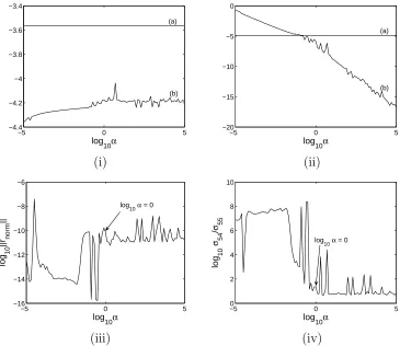
Fig. 1. (i)(a) The maximum allowable value ofkzf1k, which is equal to kf1k/µ, (b) the computed value ofkzf1k; (ii)(a) the maximum allowable value ofkzg1k/α, which is equal tokg1k/µ, (b) the computed value ofkzg1k/α; (iii) the normalised residual
krnormk; (iv) the singular value ratioσ54/σ55.
The exact polynomials (18) and (19) were perturbed by noise such that µ= 108 and then normalised by the geometric mean of their coefficients, yielding
the polynomials f1(y) and g1(y). Figure 1 shows the results of applying the
criteria in Steps 2,3 and 4 in Algorithm 4.1. In particular, Figure 1(i) shows the ratiokf1k/µ, which is the maximum allowable perturbation of f1(y), and
the variation withαof the computed value of kzf1k, which is calculated by the
method of STLN. Figure 1(ii) is the same as Figure 1(i), but for the polynomial
g1(y), and it is seen from (14) and (15) that valid solutions are obtained for
log10α > −0.9. Figure 1(iii) shows the variation of the normalised residual
krnormkwith α, and it is seen that it ranges fromO(10−16) to O(10−8) in the
specified range ofα.
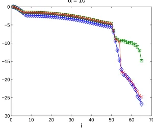
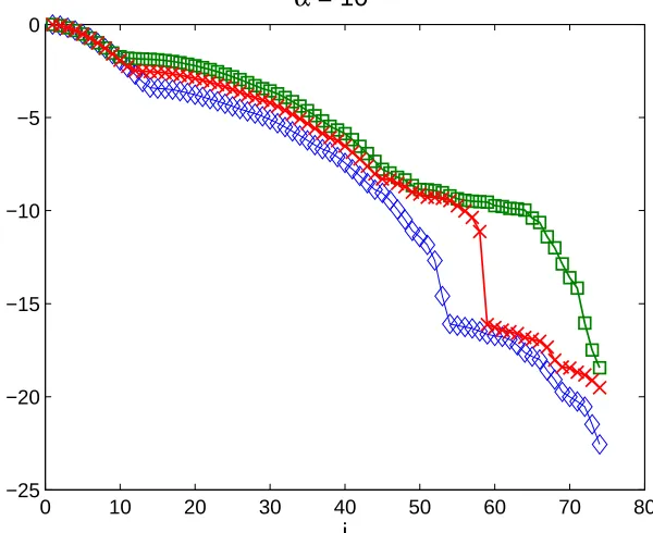
[image:16.612.101.466.96.412.2]0 10 20 30 40 50 60 70 −30
−25 −20 −15 −10 −5 0
α = 10−0.6
[image:17.612.136.436.32.283.2]i
Fig. 2. The normalised singular values of the Sylvester matrix, on a logarithmic scale, for (i) the theoretically exact dataS( ˆf1,gˆ1),♦; (ii) the given inexact dataS(f1, g1),
; (iii) the computed data S( ˜f1,0,g˜1,0), ×, forα = 10−0.6. All the polynomials are
normalised by the geometric mean of their coefficients.
in (17), and it is seen that the profile of this curve could be produced (ap-proximately) by calculating the reciprocal (to within a scale factor) of the normalised residual shown in Figure 1(iii). This result, which has been ob-served frequently, suggests that small values of the normalised residual are associated with large values of the ratio (17). It is noted, however, that a small value of the residual does not necessarily imply an accurate solution of a linear algebraic equation, and thus the use of the residual as the criterion for the acceptance or rejection of a solution is not recommended [6]. Rather, the results suggest that the residual should be used as one of several criteria for the acceptance or rejection of a solution.
This example clearly shows the importance of including α in the analysis be-cause there exist, in general, many values ofαfor which the normalised residual is sufficiently small and the ratio σ54/σ55 is sufficiently large. The small value
of the normalised residual implies that the perturbed equation (6) is satisfied to high accuracy, and the large value of σ54/σ55 implies that the numerical
rank of the structured low rank approximation S( ˜f1,g˜1) is well defined. Each
of these values of α yields a different structured low rank approximation of
S(f1, αg1), and therefore a different approximate GCD off1(y) and g1(y).
a poor solution is obtained because the ratio of the singular values (17) is approximately equal to 101.5, which is about 7 orders of magnitude smaller
than the ratio obtained for log10α = −0.6, which is the optimal value of α. Figure 1(iii) shows that if log10α = 0, the normalised residual is about 6
orders of magnitude larger than the value obtained for log10α =−0.6. These observations show that an arbitrary choice ofα can yield severely suboptimal results when it required to compute an approximate GCD of f(y) and g(y) fromS(f, αg).
Figure 2 shows the normalised singular values of the Sylvester resultant ma-tricesS( ˆf1,gˆ1),S(f1, g1), andS( ˜f1,0,g˜1,0) for the optimal value of α, where all
the polynomials are normalised by the geometric mean of their coefficients. The polynomials ˜f1,0(y) and ˜g1,0(y) are the polynomials from Algorithm 4.1
that form the structured low rank approximation ofS(f1, αg1), α = 10−0.6. It
is seen that the computed singular values ofS( ˆf1,gˆ1) do not show a sharp cut
off, which would suggest that the polynomials (18) and (19) are coprime. The profile of the singular values ofS(f1, g1) shows that the noise affects the small
singular values severely, but significantly improved results are obtained when the Sylvester matrix S( ˜f1,0,g˜1,0) is considered. In particular, it is clear that
the numerical rank of this matrix is equal to 54 because σ54 is about 7 orders
of magnitude larger than σ55. Since the Sylvester matrix is of order 65×65
andk= 11, it is seen that the method of STLN has yielded an excellent result. Convergence of the algorithm was achieved in 45 iterations. It is clear that
S( ˜f1,0,g˜1,0) can be used to compute an approximate GCD of f1(y) andg1(y).
This example has considered the situation in which the correct subresultant has been selected because the degree of the GCD of ˆf1(y) and ˆg1(y) is 11,
which is the chosen value of k, but this information is not, in general, known
a priori. It is therefore necessary to consider how the solution changes as a function of k, and this is investigated in Case 2.
Case 2: Signal-to-noise ratio µ= 108. The effects of different subresultants.
It follows from Theorem 2.1 that the lower bound on the degree of the GCD of ˆf1(y) and ˆg1(y) decreases as k decreases, and the next set of experiments
investigates the performance of the method of STLN ask changes.
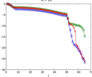
Computational experiments showed that the method of STLN is able to com-pute structured low rank approximations for k = 10, . . . ,1. Figure 3 shows the results for k = 8, and it is seen that the numerical rank of S( ˆf1,gˆ1) is
not defined, but the numerical rank of its structured low rank approximation
S( ˜f1,0,g˜1,0) is equal to 57, corresponding to a loss in rank of 8. Convergence
0 10 20 30 40 50 60 70 −30
−25 −20 −15 −10 −5 0
α = 101.4
[image:19.612.138.437.33.283.2]i
Fig. 3. The normalised singular values of the Sylvester matrix, on a logarithmic scale, for (i) the theoretically exact dataS( ˆf1,gˆ1),♦; (ii) the given inexact dataS(f1, g1),
; (iii) the computed data S( ˜f1,0,˜g1,0), ×, for α = 101.4. All the polynomials are
normalised by the geometric mean of their coefficients.
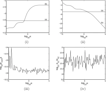
Consider now the situation that occurs for k = 12,13 and 14. In particular, successful results were obtained for k = 12 and k = 13, but the computed solution fork≥14 was not acceptable. This can be seen fork = 14 in Figures 4(i) and (ii), which show that although valid solutions exist for either f1(y)
or g1(y), they do not exist forboth f1(y)and g1(y). It is noted that if it is not
required that the solution lie in the legitimate solution space, it is possible to construct structured low rank approximations matrices that can be used for the computation of approximate GCDs off1(y) and g1(y), such that the ratio
(17) is large and the normalised residual is small. 2
The next example is only considered briefly because the important points have been discussed in the previous examples.
Example 4.2 Consider the polynomials
ˆ
f2(y) = (y−1)8(y−2)16(y−3)24,
and
ˆ
−5 0 5 −4.5
−4 −3.5 −3 −2.5 −2
(a) (b)
log
10α
(i)
−5 0 5
−14 −12 −10 −8 −6 −4 −2 0
(a)
(b)
log
10α
(ii)
−5 0 5
−16.5 −16 −15.5 −15 −14.5 −14
log
10α
log
10
||r norm
||
(iii)
−5 0 5
9.8 10 10.2 10.4 10.6 10.8 11
log
10α
log
10
σ 51
/
σ 52
(iv)
Fig. 4. (i)(a) The maximum allowable value ofkzf1k, which is equal to kf1k/µ, (b) the computed value ofkzf1k; (ii)(a) the maximum allowable value ofkzg1k/α, which is equal tokg1k/µ, (b) the computed value ofkzg1k/α; (iii) the normalised residual
krnormk; (iv) the singular value ratioσ51/σ52.
which have 16 common roots, and thus the rank ofS( ˆf2,ˆg2) is 58. The
poly-nomials were perturbed by noise such that µ= 108, and the result fork = 16
is shown in Figure 5. It is seen that although the numerical rank ofS( ˆf2,ˆg2) is
not well defined, the rank of the structured low rank approximationS( ˜f2,0,g˜2,0)
is 58, which is the correct value. Convergence was achieved in 22 iterations.2
5 Summary
[image:20.612.101.465.31.344.2]0 10 20 30 40 50 60 70 80 −25
−20 −15 −10 −5 0
α = 100.1
[image:21.612.137.437.34.279.2]i
Fig. 5. The normalised singular values of the Sylvester matrix, on a logarithmic scale, for (i) the theoretically exact dataS( ˆf2,gˆ2),♦; (ii) the given inexact dataS(f2, g2),
; (iii) the computed data S( ˜f2,0,˜g2,0), ×, for α = 100.1. All the polynomials are
normalised by the geometric mean of their coefficients.
GCD of f(y) and g(y). Additional constraints can be incorporated into the method in order to reduce further the range of acceptable values of α. Scaling the polynomials may affect the computed results, and it must therefore be chosen carefully. In this paper, scaling by the geometric mean of the coeffi-cients of the polynomials was used, and very good results were obtained. It was shown that valid approximate GCDs of two inexact polynomials must sat-isfy a bound on the magnitude of the perturbations calculated by the method of STLN, and that this bound is related to the signal-to-noise ratio of the coefficients of the inexact polynomials.
References
[1] J. Barlow. Error analysis and implementation aspects of deferred correction for equality constrained least squares problems. SIAM J. Numer. Anal., 25(6):1340–1358, 1988.
[3] S. Barnett. Polynomials and Linear Control Systems. Marcel Dekker, New York, USA, 1983.
[4] R. M. Corless, P. M. Gianni, B. M. Trager, and S. M. Watt. The singular value decomposition for polynomial systems. InProc. Int. Symp. Symbolic and Algebraic Computation, pages 195–207. ACM Press, New York, 1995.
[5] R. M. Corless, S. M. Watt, and L. Zhi. QR factoring to compute the GCD of univariate inexact polynomials. IEEE Trans. Signal Processing, 52(12):3394– 3402, 2004.
[6] G. H. Golub and C. F. Van Loan. Matrix Computations. John Hopkins University Press, Baltimore, USA, 1996.
[7] E. Kaltofen, Z. Yang, and L. Zhi. Structured low rank approximation of a Sylvester matrix, 2005. Preprint.
[8] N. Karmarkar and Y. N. Lakshman. Approximate polynomial greatest common divsior and nearest singular polynomials. In Proc. Int. Symp. Symbolic and Algebraic Computation, pages 35–39. ACM Press, New York, 1996.
[9] B. Li, Z. Yang, and L. Zhi. Fast low rank approximation of a Sylvester matrix by structured total least norm. J. Japan Soc. Symbolic and Algebraic Comp., 11:165–174, 2005.
[10] C. Van Loan. On the method of weighting for equality-constrained least squares problems. SIAM J. Numer. Anal., 22(5):851–864, 1985.
[11] V. Y. Pan. Computation of approximate polynomial GCDs and an extension. Information and Computation, 167:71–85, 2001.
[12] J. Ben Rosen, H. Park, and J. Glick. Total least norm formulation and solution for structured problems. SIAM J. Mat. Anal. Appl., 17(1):110–128, 1996.
[13] C. J. Zarowski, X. Ma, and F. W. Fairman. QR-factorization method for computing the greatest common divisor of polynomials with inexact coefficients. IEEE Trans. Signal Processing, 48(11):3042–3051, 2000.
[14] Z. Zeng. The approximate GCD of inexact polynomials. Part 1: A univariate algorithm, 2004. Preprint.