Substructuring of dynamical systems via the adaptive minimal control synthesis algorithm

This is a repository copy of Substructuring of dynamical systems via the adaptive minimal

control synthesis algorithm.

White Rose Research Online URL for this paper:

http://eprints.whiterose.ac.uk/79675/

Version: Accepted Version

Article:

Wagg, D.J. and Stoten, D.P. (2001) Substructuring of dynamical systems via the adaptive

minimal control synthesis algorithm. Earthquake Engineering and Structural Dynamics, 30

(6). 865 - 877. ISSN 0098-8847

https://doi.org/10.1002/eqe.44

[email protected] Reuse

Unless indicated otherwise, fulltext items are protected by copyright with all rights reserved. The copyright exception in section 29 of the Copyright, Designs and Patents Act 1988 allows the making of a single copy solely for the purpose of non-commercial research or private study within the limits of fair dealing. The publisher or other rights-holder may allow further reproduction and re-use of this version - refer to the White Rose Research Online record for this item. Where records identify the publisher as the copyright holder, users can verify any specific terms of use on the publisher’s website.

Takedown

If you consider content in White Rose Research Online to be in breach of UK law, please notify us by

Substructuring of dynamical systems via the adaptive

minimal control synthesis algorithm

D. J. Wagg

_{and D. P. Stoten}

Faculty of Engineering, University of Bristol, Queens Building, University Walk, Bristol BS8 1TR, U.K.

Summary

In this paper we consider the concept of modelling dynamical systems using numerical-experimental

substructuring. This type of modelling is applicable to large or complex systems, where some part of the

system is difficult to model numerically. The substructured model is formed via the adaptive minimal

control synthesis (MCS) algorithm. The aim of this paper is to demonstrate that substructuring can

be carried out in real time, using the MCS algorithm. Thus we reformulate the MCS algorithm into a

substructuring form. We introduce the concepts of a transfer system, and carry out numerical simulations

of the substructuring process using a coupled three mass example. These simulations are compared

with direct simulations of a three mass system. In addition we consider the stability of the substructuring

algorithm, which we discuss in detail for a class of second order transfer systems. A numerical-experimental

system is considered, using a small scale experimental system, for which the substructuring algorithm

is implemented in real time. Finally we discuss these results, with particular reference to the future

application of this method to modelling large scale structures subject to earthquake excitation.

KEY WORDS: adaptive control; numerical-experimental substructuring; real time control; modelling

large structures; earthquake excitation

Draft version. February 14, 2000

∗_{Research assistant. Departments of Civil and Mechanical Engineering. [email protected], TEL: +44 117}

9546832, FAX: +44 117 9287783

†_{Professor of Dynamics and Control, Department of Mechanical Engineering, [email protected], TEL:}

Introduction

The size and complexity of many dynamical systems makes accurate predictive modelling of

dy-namic behaviour difficult. This is particularly true for large scale engineering structures such as

bridges and dams, where design engineers often use experimental model testing of the structure,

in addition to theoretical and numerical modelling. Large scale testing facilities such as shaking

tables and reaction walls have been used for many years to carry out experimental modelling for

such structures?_{. However, because of size and weight limitations full scale dynamic testing is}

im-possible for most large structures. As a result, often complex experimental test results have to be

interpreted with the additional problem of scaling between the model and the full size structure.

For numerically simulating modular structures or those with a high degree of self similarity

the technique ofsubstructuring?_{has been developed to reduce the computational workload. The}

concept of subdividing a structure can also be used to formulate a model where one (or more) of

the substructures is a physical test specimen. In this case the model of the overall structure is a

combination of a numerical and an experimental model.

This type of combined modelling is particularly suitable to structures where a design critical

element can be identified. Critical elements are those which are most difficult to model

numer-ically, or most likely to fail during dynamic loading, and as such are of primary interest to the

design engineer — in other words, parts of the structure which exhibit nonlinear or unpredictable

behaviour. In this case the critical element would be modelled using a physical test specimen

while the remainder of the structure is modelled numerically. The advantage of this method over

scale model testing is that the critical element is tested at full size and the problems associated

with scaling are eliminated.

The numerical–experimental substructuring technique has been used for testing large scale

structures?_{using apseudodynamicapproach}?_{in which dilated time scales are used, so that loading}

is applied to the structure quasi-statically. These tests are often performed using reaction wall

facilities, where the reaction forces induced in the structure can be measured accurately, but real

time inertia forces have to be estimated numerically. The concept of pseudodynamic testing has

been extended to real time scales for single degree of freedom systems without substructuring?_by

using a dynamic actuator, for the purpose of testing velocity dependent components.

A more direct way of simulating the effects of dynamic loading on a structure is to use a shaking

cannot be realised by the pseudodynamic approach. By extending the concept of numerical–

experimental substructuring to real time testing, the use of shaking table facilities can give more

realistic modelling of the dynamic response of complex structures to dynamic loading?_{. This is}

the overall aim of this current research.

To produce such a combined numerical–experimental model some part of the two systems must

be synchronised using a control algorithm. Here we use the minimal control synthesis (MCS)

adaptive control algorithm?_{. This algorithm is classed as a model reference adaptive controller,}

which can be used without the need for system identification of the controlled system’s parameters.

In this current work we demonstrate how the MCS algorithm can be reformulated to form a

substructure model for a dynamical system containing nonlinear (or other unknown) elements.

In addition, using the passivity concept, we describe the stability proof for the substructured

algorithm. We also present numerical simulations of a three mass system example to

demon-strate the viability of this form of substructuring as a modelling technique. Finally we present

implementation results using an experimental system as part of a substructuring model.

Theoretical formulation

The aim of the substructuring process is to model the dynamical behaviour of the overall system

using a part numerical, part experimental model. Thus we refer to the overall system we wish to

model as the structure and the physical test specimen as the substructure. The remaining part

of the overall system is modelled numerically, and we refer to this as the numerical model. The

combined numerical-experimental model is referred to as the substructured model.

The dynamics of the structure are governed by a general system of equations

˙

w(t) =h(w, t) (1)

wherewis the state vector of the overall system,h(·) denotes an arbitrary function, and an overdot

represents differentiation with respect to timet. Effectively, the aim of the substructuring process

is to model the dynamics ofh(·). Typically, we wish to characterise the dynamic response of the

overall system subject to some excitation signalr(t), such as an earthquake.

In general, the form ofh(·) is not known explicitly, but we assume that it can be split into

linear and nonlinear parts, so that

˙

wherer(t) is the excitation signal,Gis a gain matrix,H is a matrix representing the linear part

ofh, and ˆhthe nonlinear (i.e. the difficult to model) part. To formulate a substructured model

we separate the overall system dynamics, equation 2, so that the linear dynamics are modelled

numerically, and the nonlinear dynamics are modelled using a physical test specimen.

To separate the two parts of the model, we divide the coordinatesw into a subset associated

with the nonlinear part,xc ⊂w, and those which represent the numerical model,z={z∈R2m:

z /∈xc}. Thus xc represents the state of the critical element(s) of the system. For the numerical

model, we assume that the system is second order, so them represents the degree of freedom of

the numerical system. Now equation 2 can be expressed as

   ˙ z ˙ xc   =   

H1 H2

H3 H4

      z xc   +    G1 G2   r+

  

ˆ

h1(z, xc, t)

ˆ

h2(z, xc, t)  

 (3)

The dynamics of the numerical model are linear, so ˆh1(z, xc, t) = 0. The dynamics represented

byH2xc map to a series of experimental measurements H2xc 7→Rf(t),f(t)∈Rq,R ∈ R2m×q,

wheref(t) is a vector of experimental measurements, andRis a transformation matrix. Typically

experimental measurements would consist of forces, displacements or accelerations. Note that

nonlinear dynamics could be included in the numerical model if known. Here we define “known”

as linear, and “unknown” as nonlinear for simplicity. We also assume that G2 is a null matrix,

such that the excitation is restricted to the numerical model. In addition, we restrict the size of

the excitation vectorr≤m, to be at most equal to the degree of freedom of the numerical model.

The numerical model can now be extracted from equation 3 to give

˙

z(t) =H1z(t) +G1r(t) +Rf(t) (4)

The values off(t) recorded from the experiment are included in this expression via the conversion

matrixR in place of theH2xc term.

In a similar manner, an equation for the dynamics ofxc could be extracted from equation 3.

However, as we are assuming that the nonlinearity defined by ˆh2 is unknown, this is unnecessary.

Using the experimental measurementsf(t), equation 4 becomes the substructured model of the

The control system

The numerical model and the substructure are coupled linearly by the matrixH. To simulate

this coupling between the two parts of the model, atransfer system is required which allows the

numerical and experimental parts to interact. This would typically be an experimental testing

facility such as a shaking table.

To perform a substructuring test, the substructure is mounted on the transfer system. Then

equation 4 is evaluated using a suitable numerical method, in discrete time steps, subject to the

excitationr(t). At the same time, the transfer system is driven by a control signal to track the

output from the numerical model, and f(t) is fed back into the numerical model. This process

is carried out inreal time so that appropriate inertia forces can be induced on the substructure.

As a result, accurate control of the transfer system is essential to perform realistic substructuring

tests.

In general we consider the dynamics of the transfer system to be linear and of the form

˙

x(t) =Ax(t) +Bu(t) +f(t) (5)

wherex∈R2n_{is the state vector of the transfer system,A∈R}2n×2n _andB∈R2n×p_{are constant}

matrices andu(t)∈Rp is the control signal. Thus{A, B} represents the dynamic parameters of the transfer system.

Here we are assuming thatf(t) is the vector of forces imposed on the transfer system by the

substructure, such that q = 2n. The force vector f(t) effectively acts as a disturbance on the

transfer system, and due to the coupling between the numerical model and substructure, it is

possible forf(t) to vary significantly during a test. Therefore the use of an adaptive controller is

preferable, as the effect of the disturbance on the transfer system cannot be known in advance.

The minimal control synthesis approach

The adaptive scheme adopted in this current work is the minimal control synthesis (MCS)

algorithm which has been developed at Bristol?,?. This algorithm is particularly suited to

sub-structuring for two reasons. Firstly, it is a model reference control algorithm, and the standard

reference model can be conveniently substituted for the numerical model of the substructured

system. Secondly, the algorithm requires no system identification, so that it can operate without

of the substructure and the numerical model, which are not required to be known for effective

controller implementation.

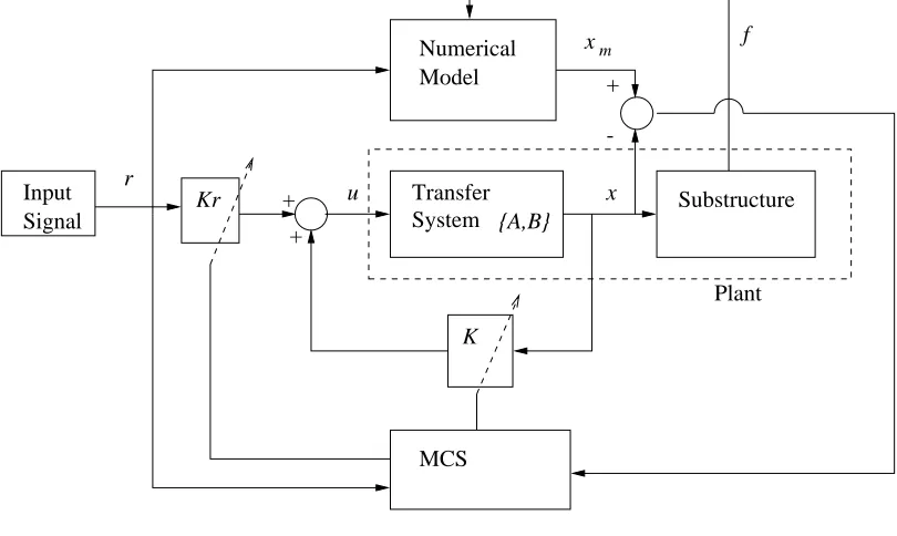
The control signal for the MCS algorithm is defined as

u(t) =K(t)x(t) +Kr(t)r(t) (6)

where r(t) ∈ Rp is the reference signal, K(t) is the feedback adaptive gain and Kr(t) the feed

forward adaptive gain. The task of the controller is to drive the transfer system to replicate the

motion of the output from the numerical model. We denote the output of the numerical model

to bexm∈R2n, wherexm⊂z,m≥n. The error signal between the required output from the

numerical model and the motion of the transfer system isxe=xm−x. This error signal indicates

the success of the control process, and as a result the overall accuracy of the method. The overall

aim of the control algorithm is that xe → 0 as t → ∞. A schematic diagram of the complete

substructuring system using MCS control is shown in Figure 1.

If z is divided into two sub-vectors such that z = [zm, xm]T, where dim(xm) = 2n×1 and

dim(zm) = (2m−2n)×1. Then equation 4 can be written in the form    ˙ zm ˙ xm   =   

H11 H12

H13 H14

      zm xm   +    G11 G12   r+

   R1 R2  

f (7)

Now ˙xm represents the “reference model” dynamics, and ˙zm represents the remaining numerical

model dynamics. Extracting the reference model dynamics from equation 7 gives

˙

xm(t) =H13zm(t) +H14xm(t) +G12r(t) +R2f(t) (8) whereH13is an 2n×(2m−2n) matrix,H14is 2n×2n,G12is a 2n×pmatrix andR2is a 2n×2n

matrix. To standardise the notation with the conventional MCS formulation let Am = H14, Bm=G12,Hm=H13 andRm=R2. Then equation 8 can be expressed as

˙

xm(t) =Amxm(t) +Bmr(t) +Hmzm(t) +Rmf(t) (9)

which is similar to the standard MCS reference model form with the addition of theHmzm(t) and

Rmf(t) terms. If we subtract equation 5 from equation 9, substituting for u(t) from equation 6,

the error dynamics of the system are given by

˙

xe=Amxe+ (Am−A−BK)x+ (Bm−BKr)r+d (10)

whered(t) =Hmzm+ (Rm−I)f(t) is considered to be a disturbance. In fact, this disturbance

from the substructure. Therefore this is an internal rather than an external disturbance for the

substructured system. Other than this, equation 10 is now in a standard form for MCS error

dynamics subject to a disturbance.

We also note that if Rm =I2n, which it does in this case where we have assumed thatf(t)

is exactly the vector of forces experienced by the transfer system, then d(t) = Hmzm. So, in

this case the disturbance comes entirely from coupling within the numerical model. Furthermore,

as the dynamics of the numerical model are linear, we can see that if the system is stable, the

disturbanced(t) is always bounded.

Stability via passivity

The stability of the error dynamics given in equation 10 can be proven using the concept of

passivity?_{. For completeness we outline the main elements of the proof here.}

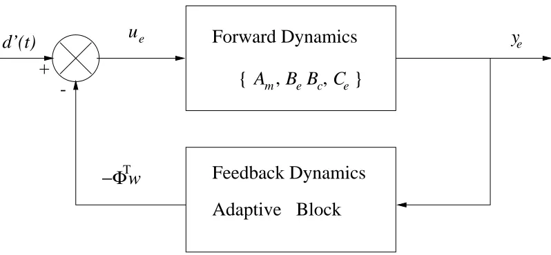
The error dynamics of the system can be divided into forward and feedback adaptive dynamic

blocks. This is illustrated schematically in Figure 2. In the figure, the system is driven by

the disturbance signal d(t), and the feedback dynamics are represented by ΦT_{w, where Φ =}

[B−1

(Am−A−BK) | B−1(Bm−BKr)] and w = [xT, rT]T. The forward dynamics of the

error system are given by

˙

xe=Amxe+BeBcue, ye=Cexe, ue= ΦTw+d

′

, (11)

where Ce is a linear compensation matrix which ensures that the triple {Am, Be, Ce} is strictly

positive real,Be= [On, In]T,Bcis ann×nmatrix andd′=B−1d. For a class of transfer systems

ge(s) between ue and ye such that ye=ge(s)Bcue, whereBc is positive definite symmetric, the

forward dynamics can be shown to be dissipative?_{. Then by proving that the dynamics of the}

adaptive block are passive via the Popov criteria

Z

ye(−ΦTw)≥ −γ

2

(12)

where γ is a finite constant, the complete system can be shown to be asymptotically stable?_.

Additional detailed information on the stability and robustness of the MCS algorithm is given

Stability of second order linear transfer systems

The transfer systems we will consider take the form of a second order mechanical oscillator,

represented by a generalised coordinateq∈Rn_{, in the form}

Mtq¨+Dtq˙+Ktq=Kau (13)

where, Mt, Dt and Ktare the mass, damping and stiffness matrices of the transfer system, and

Ka is the actuator gain. For this system, the mass matrix,M, is positive definite by definition.

In addition we will assume that by design,Ka can be taken as positive definite, and that all the

parameter matrices are symmetric. For a transfer system in this Lagrangian form, equation 11

has coefficient matrices

A=

  

0n In

−M−1

t Kt −M

−1

t Dt  

, B=   

0

M−1

t Ka  

 (14)

in Lagrangian coordinate form. The matrixBcan be written asB =BeBc, whereBe= [On, In]T

and Bc = M−

1

Ka is a positive definite symmetric matrix. The plant matrix for the reference

model,Am, is of a similar structure to theAmatrix, and is chosen to be stable, such that all the

eigenvalues ofAm have negative real parts. For a substructuring system, Am is a subset of the

numerical model, so this condition places a restriction on the class of numerical models which can

be used. If requiredKa can be included as part of the feedback dynamics?.

The transfer function ge(s) between ye(s) and ue(s) is Ce(sI −Am)−1Be, such that ye =

ge(s)Bcue. For this class of transfer systems, Ce can be chosen so that ge(s) is strictly positive

real, and hence the forward dynamics of equation 13 are dissipative.

Numerical example

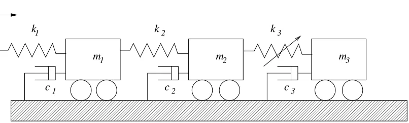
We now consider a numerical example of a three mass oscillator system, which is shown

schemat-ically in Figure 3. This system is one of the simplest configurations which can be used to

demon-strate the substructuring concept. The three masses are coupled by two linear springsk1 andk2,

and a nonlinear springk3. Each mass is independently damped by a viscous damperci,i= 1,2,3.

The system is forced via a support motionr(t). Here we will compare the output from a direct

simulation of the system with the output of a substructured model of the system, to demonstrate

can be written as

Mξ¨+Dξ˙+g(ξ) =Sr(t) (15)

where,M andD are the mass, and damping matrices respectively, the stiffness is represented by

g(ξ) andSr(t), represents the support excitation. Equation 15 represents the structure we wish to

model, and can be expressed in first order form (as equation 1), where ˆh1(w, t) = 0, and ˆh2(w, t)

represents the stiffness function,g(ξ). In this example we will use a cubic spring nonlinearity in

addition to a linear stiffness term to formg(ξ).

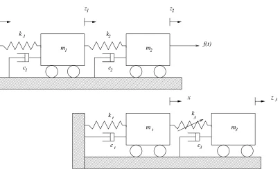
To model this overall system we split it into a numerical model and substructure, which is

shown, schematically, in Figure 4. Here, we have chosen massm3 as the substructure, since k3

is the nonlinear part of the structure. This is mounted on the transfer system, massmt, which

has stiffnessktand dampingct. The massesm1andm2 correspond to the numerical model. The effect ofm3 onm1 andm2 is now represented by the single measurementf(t) which in this case

is a force. Note that selectingm1 or m2as the substructure is more difficult. This would involve

having two transfer systems, which experimentally would be more difficult to implement. We

envisage that this type of system will form the subject of future work, especially with regard to

the multiple support excitation of structures?_.

Writing the numerical model dynamics in the form of equation 4, gives

˙

z=

  

0m Im

−M−1

Ks −M

−1 D

  z+

  

0m

M−1 S

  r(t) +

   0m I  

f(t) (16)

where we have used the Lagrangian formulation such thatz∈R4

= [z1, z2,z˙1,z˙2]T. Also

M =

  

m1 0

0 m2

  , Ks=

  

k1+k2 −k2

−k2 k2

 

, D=   

c1 0

0 c2

 

, S =   

k1 0

0 0

 

 (17)

For this example, we see that by synchronising the motion ofm2 andmt using the control

algo-rithm, the motion ofm1, m2 and m3 should be the same for both the complete system, Figure

3, and the substructured model, Figure 4. The forcef(t) =k3((z3−x) + (z3−x) 3

) +c3z˙3 can

be computed (rather than measured) at each iteration, and it includes the effect of the nonlinear

spring.

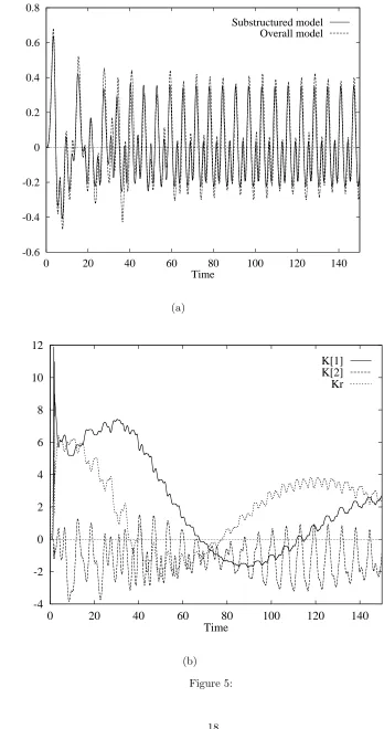
To compare the output of the two systems, we monitor the displacement of massm2 and the

transfer system mass,mt. The displacementxof the massmtof the substructured system forced

Figure 5 (a) shows the displacement of massm2 of the overall system, Figure 3, using the same

forcing.

It is worth emphasising that the output from the substructured model is not connected with

the direct simulation of the three mass system in any way. So, in Figure 5 (a) we are plotting the

output from two completely separate numerical systems. There is a good level correlation between

the two signals, indicating that in this case the substructured model is a close representation of

the overall system. We do not attempt to quantify the level of correlation between the two

systems here. However, we note that the nonlinear nature of the systems means that during

transient motion the dynamics are sensitive to small perturbations. As a result the dynamics of

the substructured model may diverge from the overall system dynamics during transient motion,

although steady state dynamics should converge (assuming that the initial conditions of both

systems are suitably far from any basin of attraction boundaries). This aspect of the modelling

procedure requires future investigation. The MCS adaptive gains are shown in Figure 5 (b). The

gain signals are composed of several oscillatory components. This is typical of adaptive gains

controlling a nonlinear system.

Numerical–experimental example

Having demonstrated the substructuring concept using a purely numerical simulation, we now

consider a true numerical–experimental system. Again we use the example of the three mass

system shown in Figure 3. In this case we formulate a substructure model of the three mass

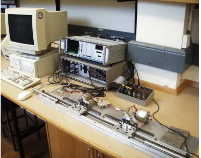
system using a numerical two mass model and aphysical two mass system. A photograph of the

experimental setup for the physical two mass system is shown in Figure 6.

The masses are mounted on a uniaxial track with wheel bearings. Springs between the two

end stops and the masses themselves provide the restoring forces for the central position of the

masses. In this system the nonlinearity occurs due to friction in the bearings on which the masses

oscillate. In this configuration one of the masses of the physical apparatus is used as the transfer

system. The position of this mass (mt) is represented by the scalar coordinate, x and can be

controlled via an electric motor. The second mass is chosen as the substructure (i.e equivalent

tom3), and is allowed to vibrate freely. The displacement of the substructure is represented by

the scalar coordinatexc. The displacements, xand xc and velocities ˙xand ˙xc of the masses are

Amplicon PC30AT card, which was also used to output the control signal. A second order MCS

controller was used which had gain wind-up protection?_{. This was implemented on a 486 Personal}

Computer running RedHat Linux 5.1 The substructuring algorithm ran at a sampling rate of

512Hz, using the Linux real-time clock.

The numerical part of the model used for this system, was similar to the example in previous

example. Two masses were coupled by springs and damped independently, with displacement

coordinatesz1 andz2. Parameters used were those of the physical system for the masses, 0.515

kg each , and spring stiffness which was measured as 2.43 N/m. Viscous damping was assumed

for the model, and a value of 2.4 Ns/m was estimated to be approximately equivalent to the

frictional damping in the physical system, for the range of forcing frequency used during testing.

The reference output from the numerical model was taken asz2, such that xm=z2.

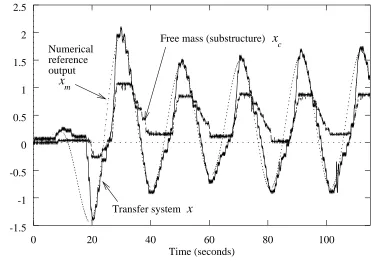
The system was forced using a low frequency sine wave, 0.1 cos(0.1t), to remain within the

limits of the computer/acquisition hardware. The results of a typical test are shown in Figure

7. In Figure 7 the amplitude of displacement of the transfer system,x, is plotted along with the

output from the numerical model,xmand the displacement of the free mass, xc. We see that for

this set of parameter values, the controlled motion has some nonsmooth characteristics due to the

frictional nature of the system. Despite this, in general the tracking is good. The effect of the

free mass on the transfer system can be seen on the upward side of the response peaks, where the

response of the transfer system is pulled away from the reference output.

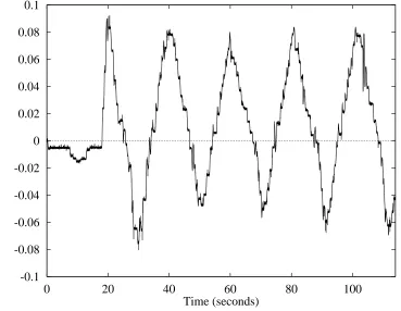
The experimental two mass rig was fitted with three relatively light springs between the masses,

which each had a stiffness of approximately 2.43 N/m. As a result the force feedback between the

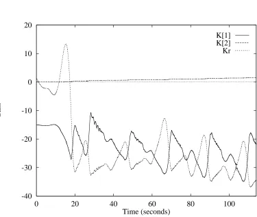
transfer system and substructure was quite low. This can be seen in the feedback force signal,

which for this test is shown in Figure 8. The MCS gains for this test are shown in Figure 9. Again

we note the periodic oscillation which occurs in the gains for a nonlinear system.

It is interesting to note that in this example, the transfer system was subject to the same

nonlinearity as the substructure. However, the MCS controller was still effective in tracking the

required signal.

Conclusions

In this paper, we have discussed the concept of numerical-experimental substructuring. For a

how a substructured model can be formulated. A key aspect of such a system is the control system.

We have used the minimal control synthesis (MCS) algorithm, which, because of its adaptive form,

is particularly suited to substructuring. We have shown how the algorithm can be reformulated

for substructuring, by substituting the standard reference model with the numerical model. When

the transfer system is in the form of a second order mechanical oscillator, we have shown via the

passivity theorem, that the system is asymptotically stable.

Using numerical simulations, we have demonstrated the concept of using a substructured model

of a three mass system. The results from this system were compared to a direct simulation of the

overall system, and a good level of agreement was observed. This demonstrates the viability of

substructuring as modelling technique. However we have noted that the correlation between the

output of the two numerical simulations is not unity due to the presence of nonlinearities. Future

work is required to determine the accuracy of the substructured model, perhaps based on the error

signal from the control algorithm. We have also shown results from a true numerical-experimental

substructured system, which demonstrates the practical application of the substructuring

algo-rithm.

In terms of modelling large scale structures, this work represents an initial step toward

de-veloping useful testing methods. We envisage future work will involve extending these results

to large scale testing facilities, such as shaking tables. In such a testing environment it should

be possible to use real time numerical–experimental substructuring to provide useful modelling

results for large scale engineering structures.

Acknowledgements

This work was funded by DG12 of the European Commission as part of the HCMP-TMR-RTD

research program in earthquake engineering, specifically grant No. ERBFMGECT-980103. In

addition the authors would like to thank Eduardo Gom´ez Gom´ez for his assistance with the

Figure Captions

• Figure 1: Schematic representation of numerical experimental substructuring system with

MCS control.

• Figure 2: Schematic representation of error dynamics as a feedback system.

• Figure 3: Schematic representation of a three mass system.

• Figure 4: Schematic representation of the substructured system used to model the three

mass system in Figure 3.

• Figure 5: Three degree of freedom system, parameter values mi = 1.0 and ci = 0.1 for

i= 1,2,3,mt = 1.0, kt = 1 and ct = 1.0. The stiffness k1 =k2 = 1.0, andk3 =−δ+δ3 whereδis the extension of the spring. A settling time of 0.01 was required and the step size

used in the Runge-Kutta algorithm was 0.001. (a) Displacement of z2of three mass system

(dashed line) plotted against x from the substructured system (solid line). (b) Adaptive

gains from the MCS algorithm,K1 solid line,K2long dashes andKr short dashes.

• Figure 6: Experimental two mass system.

• Figure 7: Displacement time series from two mass substructuring test showing output from

the numerical model, xm, displacement of the transfer system,x, and displacement of the

free massxc. Sample rate 512Hz.

• Figure 8: Feedback force from two mass substructuring test. Sample rate 512Hz.

MCS Kr

K

x

x_m

+

+

+

-Substructure Model

Numerical f

u Transfer

Plant Input

Signal r

System {A,B}

+

-Feedback Dynamics

Adaptive

Forward Dynamics

B

y

−Φ

w

u

Block

d’(t)

e

B

C

}

{ A

’

’

0000000000000000000000000000000000000

0000000000000000000000000000000000000

0000000000000000000000000000000000000

1111111111111111111111111111111111111

1111111111111111111111111111111111111

1111111111111111111111111111111111111

m

m

m

1 2

2 3

k

r

2

c

c

1

c

k

k

-0.6 -0.4 -0.2 0 0.2 0.4 0.6 0.8

0 20 40 60 80 100 120 140

Amplitude of response

Time

Substructured model Overall model

(a)

-4 -2 0 2 4 6 8 10 12

0 20 40 60 80 100 120 140

Gain amplitude

Time

K[1] K[2] Kr

(b)

-1.5 -1 -0.5 0 0.5 1 1.5 2 2.5

0 20 40 60 80 100

Voltage

Time (seconds) Free mass (substructure)

Transfer system

x

x

m

x

c

Numerical reference output

-0.1

-0.08

-0.06

-0.04

-0.02

0

0.02

0.04

0.06

0.08

0.1

0

20

40

60

80

100

Newtons

Time (seconds)

-40

-30

-20

-10

0

10

20

0

20

40

60

80

100

Gain

Time (seconds)

K[1]

K[2]

Kr