Article
On Computing the Worst-case
Performance of
Lur'e Systems with Uncertain Time-invariant Delays
Thapana Nampradit and David Banjerdpongchai
*
Department of Electrical Engineering, Faculty of Engineering, Chulalongkorn University, 254 Phayathai Road, Pathumwan, Bangkok 10330, Thailand
*E-mail: [email protected]
Abstract. This paper presents a worst-case performance analysis for Lur'e systems with time-invariant delays. The sufficient condition to guarantee an upper bound of the worst-case performance is developed based on a delay-partitioning Lyapunov-Krasovskii functional containing an integral of sector-bounded nonlinearities. Using Jensen inequality and -procedure, the delay-dependent criterion is given in terms of linear matrix inequalities. In addition, we extend the method to compute an upper bound of the worst-case performance of Lur'e systems subject to norm-bounded uncertainties by using a matrix eliminating lemma. Numerical results show that our criterion provide the least upper bound on the worst-case performance comparing to the criteria derived based on existing techniques.
Keywords: Worst-case performance, Lur'e systems, time-invariant delay, Lyapunov-Krasovskii functional, linear matrix inequality (LMI).
ENGINEERING JOURNAL Volume 19 Issue 5 Received 23 September 2014
1.
Introduction
Lur'e systems [1] are nonlinear systems described by linear dynamic systems with feedback through sector-bounded nonlinearities. Such nonlinearities can be used to capture many common characteristics such as saturation, dead zone and spring stiffness. In addition to nonlinearities, time delays are frequently encountered in dynamic systems. The detrimental effects of time delays on system stability and performance are well known. Therefore, the studies on Lur'e systems with time delays (LSTD) are of theoretical and practical importance.
In the recent years, many studies have applied Lyapunov-Krasovskii Theorem [2] to develop absolute stability analysis for LSTD. In particular, various types of Lyapunov-Krasovskii functional (LKF) are used to formulate sufficient conditions. We can classify the stability conditions into two categories. The first is delay-independent criteria [3, 4], which provide the sufficient condition regardless of time delays. The second is delay-dependent criteria [5–12], which use the information on the delay length to prove the stability. Delay-independent criteria are quite limited in providing conclusion for the systems whose stability depends on the time delay. Therefore, subsequent studies concentrate on developing delay-dependent criteria. In [5], a model transformation and a bounding technique [13] are used to formulate the delay-dependent stability criterion. The drawback is that the upper bound of the cross product terms may not be tight and can lead to a conservative criterion. Later, a free weighting matrices (FWM) approach proposed by [6] applies relationship between each term in the Leibniz-Newton formula to the stability criterion. Although a bounding technique is not required for this approach, it introduces some slack variables apart from the matrix variables in the LKF. Motivated by [14], Jensen inequality is employed to derive absolute stability criteria for LSTD [7, 8]. It is shown in [15] that the FWM approach and Jensen inequality produce the identical results and conservatism, but the latter technique requires less number of decision variables.
Recently, several researchers proposed novel methods to analyze the absolute stability of LSTD based on the discretization scheme [14, 16]. They include delay-decomposition approach [17], -segmentation method [9, 12], and delay-dividing approach [10]. The principle of these methods is to divide an interval
into equidistant partitions, and the LKF is separated corresponding to each subinterval of delay. Then, the Jensen inequality or the FWM approach is utilized to formulate the stability criterion in terms of linear matrix inequalities (LMIs). These methods successfully reduce conservatism of the stability criteria comparing to previous techniques. Moreover, it is proved that the conservatism of the criteria can be further reduced by increasing the number of partitions [18]. Among these criteria, [9], [11] and [12] proposed the absolute stability analysis for LSTD with a time-invariant delay. In [9], the delay interval is partitioned into equidistant fragments, and the stability criterion is formulated by using Jensen inequality. However, the LKF used in [9] does not contain an integral of nonlinearities, which is essential for stability analysis of LSTD. In [11], the delay interval is divided into two specific subintervals, namely,
and , and the criterion is developed by using integral-equality technique, which is, in fact, another form of FWM approach. Although the LKF based on [11] utilize the integral of nonlinearities, their delay interval is only divided into two fixed subintervals, which is too specific. Recently, [12] fulfilled this gap by developing an improved absolute stability by combining the delay partitioning approach with utilizing integral terms involving sector-bounded nonlinearities in the LKF. The numerical results confirm that the criterion in [12] provides substantial improvement comparing to those in [9] and [11] especially when the sector bound is comparatively large.
The worst-case performance is defined by -gain of the nonlinear systems. A Lyapunov-Krasovskii functional can be incorporated with an upper bound of the -gain to calculate an upper bound of such worst-case performance; see [19] for sector-bounded nonlinearities, and [20] for another type of uncertainties. To the best of our knowledge, there is a few works on how to compute an upper bound of the worst-case performance for LSTD [21]. It is worth developing the worst-case performance criterion based on the combination of delay partitioning approach and employing the Lyapunov functional terms involving integral of nonlinearities. With the new performance analysis criterion, we can approach the actual value of the worst-case performance.
is formulated in terms of LMI by eliminating an uncertain matrix. In addition, we also develop two performance analysis criteria along with the concept presented in [9] and [11], and use them as the comparative criteria.
The paper is organized as follows. Section 2 introduces the notations and reviews the relevant lemmas. The definition of the worst-case performance and analysis are first stated in section 3. In section 4, the worst-case performance criteria for both nominal and uncertain LSTD are presented. Section 5 shows the numerical results and compares the upper bounds of the worst-case performance between the proposed criterion and the comparative criteria. Finally, Section 6 provides the summary of the main results and gives conclusions.
2.
Preliminaries
is the set of nonnegative numbers, and is the set of real -vectors. and denote a vector with all entries one and a vector with all entries zero of appropriate order, respectively. is the vector space of real matrices. For any matrix , denotes its transpose. and are an identity matrix and a null matrix of appropriate dimensions, respectively. The notation is used for diagonal matrices. For symmetric matrices and , the notation means that matrix is positive definite (positive semi-definite). Furthermore, for an arbitrary matrix , and two symmetric matrices and
, the symmetric term in a symmetric block matrix is denoted by *, i.e.,
is the Hilbert space of square-integrable signals defined over with -components; is often abbreviated as . The symbol stands for the norm.
The notation represents a vector of nonlinearities, which belong to the set characterized by memoryless, time-invariant nonlinearities satisfying certain sector conditions. In particular, given an input
vector , a lower bound vector and an upper bound vector
, with for all , the set can be described as follows
.
Finally, the following lemmas are useful for establishing the worst-case performance criteria.
Lemma 1 (Jensen Inequality) [14] For any constant matrix , , scalar , vector function such that the integrations concerned are well defined, then
Lemma 2 [22] Given matrices , , and of appropriate dimensions and with and symmetrical and , then
for all satisfying
3.
Problem Statement
We consider Lur'e systems with unknown time-invariant state delay described as follows.
(1)
with and zero initial condition , , is a time-invariant time delay in the state. The notation is the state variable, is the disturbance input which belongs to , is the performance output, , and are the input/output of a vector mapping of sector-bounded nonlinearities denoted by . In addition, the pairs and are assumed to be controllable and observable, respectively. Next, the definitions of -stability and the worst-case
performance for the system (1) are introduced.
Definition 1 ( -stable) A causal operator is said to be -stable if there exist and such that
Definition 2 (Worst-case Performance) Assume that the system (1) is -stable with finite gain and zero bias. The worst-case performance of the system (1) is defined by its -gain described as follows.
(2)
where the supremum is taken over all nonzero output trajectories of the system (1) under zero initial condition.
While the actual value of is difficult to compute, its upper bound, such that , can be calculated from the following minimization problem [19].
minimize subject to
where denotes the Lyapunov functional candidate. Therefore, the worst-case performance analysis problem is to determine an upper bound of of the system (1) for any time-invariant time delay
, i.e., for a given , determine such that .
In addition, we consider the LSTD with norm-bounded uncertainties described as follows.
(3)
with . The uncertain variables , , and are time-varying, but norm-bounded. The uncertainties are assumed to be of the following form
where , , , and are known constant real matrices of appropriate dimensions, and represent the structure of uncertainties, and is an unknown matrix function with Lebesgue measurable elements satisfying the constraint Similar to the nominal system (1), the worst-case performance analysis problem for the uncertain system (3) is to determine an upper bound of of the system (3) with any time-invariant time delay , and for given matrices corresponding to norm-bounded uncertainties, i.e., , , , and .
4.
Worst-case
Performance Analysis
In this section, we present a sufficient condition for computing an upper bound of the worst-case performance, which is derived by means of a Lyapunov-Krasovskii functional. Accordingly, the choice of LKF candidate plays a crucial role in developing the computing criterion. We employ the delay partitioning technique to the LKF for the system (1). The idea of this method is to divide the interval into
number of partitions, i.e., , where , and separately
define the LKF involving delay on each subinterval. Consider the LKF candidate of the form
(5)
with
where , , and are positive definite symmetric matrices of dimension , scalars are non-negative, and denotes a piece of trajectory for . Next, we will show how to calculate the upper bound for the nominal LSTD (1).
Theorem 1 For a given , an upper bound of the worst-case performance of LSTD (1) for any time-invariant time delay can be computed by minimizing subject to the constraint (6) over
symmetric matrices , , for all , and diagonal matrices , .
(6)
with .
Proof: Assume that is Hurwitz, and system matrices are minimal realization. If there exists an LKF of the form (5) and such that
(7)
for all satisfying the system equations (1), then . Therefore, we seek , , , and such that the constraint (7) is satisfied for all nonzero satisfying (1) with a set of sector-bounded conditions
(8)
To verify (7) under the set of constraints (8), we apply -procedure [23] to establish the sufficient condition as follows.
(9)
where . Note that for the case of single nonlinearity ( ), -procedure is lossless, and the condition (9) is not only sufficient but also necessary for (7). By defining , the inequality (9) can be written in vector-matrix notation as follows.
(10)
The derivative of each term in the LKF (5) with respect to time along the solution of (1) is given by
(11)
where , and employ Lemma 1 (Jensen inequality) to bound the
integral terms appeared in as follows.
(12)
where , and the entries left blank are zero. Substituting , , and into inequality (10), and applying (11) and the upper bound (12) for , the sufficient condition for (10) is given as follows.
(13)
where , and
(14)
Inequality (13) holds for all if and only if the following matrix inequality is satisfied.
(15)
Lastly, applying Schur complement [19, pp.7–8] and substituting with , we obtain inequality (6).
It is important to note that the sufficient condition (6) guarantees an upper bound for the case of . Next, we show that (6) also guarantees the same for the system (1) for any time-invariant time delay . Let , where . Clearly, lies in the interval . By substituting with , and isolating all terms involving , the matrix inequality (14) becomes
(16)
Theorem 1 guarantees an upper bound for the systems (1) for any time-invariant time delay .
This completes the proof. █
It is appeared that the condition (6) is LMI over matrix variables , , , , and for a given . Hence, the problem of minimizing subject to (6) can be cast as a minimization problem with LMI constraints which can be solved efficiently.
Remark 1 In Theorem 1, it is straightforward to handle general sector condition . By using loop transformation [24], LSTD (1) with can be transformed to an equivalent LSTD with . In particular, define
It is easy to show that for all , i.e., . Let ,
, and . We then substitute into (1),
and obtain the equivalent LSTD systems as follows.
(17)
with , where and . Note that the transformed LSTD (17) is
equivalent to the original LSTD (1), and we can calculate an upper bound for LSTD (1) by considering the system (17).
Next, we will derive another sufficient condition for computing an upper bound of for the uncertain LSTD (3).
Theorem 2 For a given , an upper bound of the worst-case performance of the systems (3) for any time-invariant time delay can be computed by minimizing subject to the constraint (18)
over symmetric matrices , , for all , and diagonal matrices , ,
and a scalar variable .
(18)
where
Proof: By applying Theorem 1 to the uncertain systems (3), the worst-case performance criterion consists of the following LMI.
(19)
where is defined as
It follows from Lemma 2 that the matrix inequality (19) is true for all uncertain matrix satisfying if and only if there exists a scalar such that
(20)
Absorbing the last term into and applying the Schur complement [19], the matrix inequality (18) holds.
This completes the proof. █
Remark 2 It is observed that the terms involving and in the matrix inequality (20) are all positive. Then, the feasible set for (18) is smaller than that of (6), and the obtained for the uncertain LSTD (3) should be greater than or at least equal to that for the nominal LSTD.
In order to illustrate the effectiveness of the proposed criteria, we develop worst-case performance analysis criteria for uncertain LSTD along with the -segmentation technique in [9] with and the integral-equality approach in [11] as stated in Theorem 3 and Theorem 4, respectively.
Theorem 3(Extension of Wu et al. (2009)) For a given , an upper bound of the worst-case performance of the systems (3) for any time-invariant time delay can be computed by minimizing subject to the constraint (21) over symmetric matrices , , , ,
, , , and scalar variables and .
(21)
and
Theorem 4(Extension of Qiu & Zhang (2011)) For a given , an upper bound of the worst-case performance of the systems (3) for any time-invariant time delay can be computed by minimizing subject to the constraint (22) over symmetric matrices , , , , , full matrices , , , , , , , , a diagonal matrix , and scalar variables and .
(22)
Remark 3 The comparative criteria can be considered as special cases of the proposed criterion in Theorem 2, i.e.,
The criterion presented in Theorem 3 is a special case of Theorem 2 when , , and
for .
Since FWM approach and Jensen inequality approach produce the stability criteria at the same level of conservatism [15], the criterion presented in Theorem 4, which utilizes a form of FWM approach, namely integral-equality approach, is as conservative as a special case of Theorem 2
when , , , and for .
The criterion proposed in [21] is a special case of Theorem 2 when .
Clearly, the conservatism of the proposed criterion is less than or at least equal to those of the comparative criteria. The additional free variables can be potentially the key to establish the less conservative criterion.
4.
Numerical Results
The conservatism of the proposed criterion in Theorem 2 with , the extension of [9] in Theorem 3, and the extension of [11] in Theorem 4 are compared on three numerical examples. The LMI Lab [25] which employs the projective interior-point method [26], is used for solving the LMI minimization problems in the experiments.
Example 1: Consider the system of the form (3) with the following parameters.
where characterizes the sector bound of nonlinearity, and represents magnitude of the uncertainty. The system data is taken from [7] with slight modifications. The uncertainty model , , and
can be described by (4) with , , , where , . Loop
transformation is applied so that LSTD with is transformed into an equivalent
LSTD with .
, , and satisfying LMI (18). With the same parameters, the minimal computed using Theorem 3 is for the following matrices
, and satisfying LMI (21). Finally, the minimal obtained from Theorem 4 is with the matrices
, , and satisfying LMI (22).
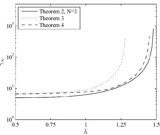
[image:12.595.156.428.493.726.2]Fig. 2. Upper bounds of for Ex. 1 when and .
Fig. 3. Upper bounds of for Ex. 1 when and .
[image:13.595.154.433.84.316.2] [image:13.595.148.434.369.606.2]Example 2: Consider the uncertain LSTD of the form (3) with the following parameters.
This example is modified from the system given in [7]. Similar to the previous example, the norm-bounded uncertainty can be described by (4) with , and are identity matrices of appropriate dimension, and is a null matrix, where , . Loop transformation is applied so that LSTD with defined above is transformed to an equivalent LSTD with .
For this example, we let , , and . The minimal provided by using Theorem 2 is with
and satisfying LMI (18). Next, the minimal calculated using Theorem 3 is with
, and .
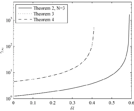
The computed versus , , and for Ex. 2 are shown in Figs. 4–6, respectively. It can be seen that Theorem 2 always give the less conservative result than those obtained from other criteria. In addition, Theorem 2 is capable of finding for a wider range of parameters, which indicate that the proposed criterion has the advantage over the comparative criteria.
Fig. 4. Upper bounds of for Ex. 2 when and .
[image:15.595.152.431.208.444.2] [image:15.595.153.432.492.731.2]Fig. 6. Upper bounds of for Ex. 2 when and .
Example 3: Consider the uncertain system of the form (3) with the following parameters.
The uncertainty matrices , and can be represented with Eq. (4) where
and , . This example is modified from the LSTD given in [8]. Again, loop transformation is applied so that LSTD with defined above is transformed to an equivalent LSTD with . Note that the new and are the zero and identity matrices of dimension , respectively.
[image:16.595.153.434.81.318.2], and satisfying LMI (18). By Theorem 3, the minimal is obtained with
, , and satisfying LMI (21). Finally, the minimal is
computed using Theorem 4 when LMI (22) is satisfied by
, , and .
[image:17.595.152.433.514.747.2]Fig. 8. Upper bounds of for Ex. 3 when and .
Fig. 9. Upper bounds of for Ex. 3 when and .
[image:18.595.153.431.85.316.2] [image:18.595.155.434.369.606.2]5.
Conclusions
In this paper, we present the worst-case performance criteria for Lur'e systems with uncertain time-invariant delays. The delay partitioning technique is applied and the information of sector-bounded nonlinearities is incorporated into the LKF in terms of integral of nonlinearities. The sufficient condition to ensure the worst-case performance is derived using Jensen inequality and -procedure. The performance criterion is formulated as a linear objective minimization problem over LMIs, which can be solved efficiently. In addition, the criterion for LSTD subject to norm-bounded uncertainties is developed by eliminating an uncertain matrix. Numerical examples show that the proposed criteria are less conservative than the comparative criteria, and can be served as an effective worst-case performance analysis for LSTD.
Acknowledgment
The authors are supported by the Thailand Research Fund through the Royal Golden Jubilee Ph.D. Program under Grant No. PHD/0148/2003, which is greatly appreciated.
References
[1] A. I. Lur'e and V. N. Postnikov, “On the theory of stability of control systems,” Applied Mathematics and Mechanics, vol. 8, no. 3, pp. 246–248, 1944. (in Russian).
[2] N. N. Krasovskii, Stability of Motion, Stanford CA, USA: Stanford University Press, 1963. (translation by J. Brenner)
[3] P. A. Bliman, “Lyapunov-Krasovskii functionals and frequency domain: Delay-independent absolute stability criteria for delay system,” International Journal of Robust and Nonlinear Control, vol. 11, pp. 771– 788, 2001.
[4] Y. He and M. Wu, “Absolute stability for multiple delay general Lur’e control systems with multiple nonlinearities,” Journal of Computational and Applied Mathematics, vol. 159, pp. 241–248, 2003.
[5] L. Yu, Q. L. Han, S. Yu, and J. Gao, “Delay-dependent conditions for robust absolute stability of uncertain time-delay systems,” in Proceedings of the 42nd IEEE Conference on Decision and Control, Maui, Hawaii, USA, 2003, pp. 6033–6037.
[6] Y. He, M. Wu, J. H. She, and G. P. Liu, “Robust stability for delay Lur’e control systems with multiple nonlinearities,” Journal of Computational and Applied Mathematics, vol. 176, pp. 371–380, 2005.
[7] Q. L. Han, “Absolute stability of time-delay systems with sector-bounded nonlinearity,” Automatica, vol. 41, pp. 2171–2176, 2005.
[8] S. Xu and G. Feng, “Improved robust absolute stability criteria for uncertain time-delay systems,” IET Control Theory & Applications, vol. 1, no. 6, pp. 1630–1637, 2007.
[9] M. Wu, Z. Y. Feng, and Y. He, “Improved delay-dependent absolute stability of Lur’e systems with time-delay,” International Journal of Control, Automation, and Systems, vol. 7, no. 6, pp. 1009–1014, 2009. [10] F. Qiu, B. Cui, and Y. Ji, “Delay-dividing approach for absolute stability of Lurie control system with
mixed delays,” Nonlinear Analysis: Real World Applications, vol. 11, pp. 3110–3120, 2010.
[11] F. Qiu and Q. Zhang, “Absolute stability analysis of Lurie control system with multiple delays: An integral-equality approach,” Nonlinear Analysis: Real World Applications, vol. 12, pp. 1475–1484, 2011. [12] T. Nampradit and D. Banjerdpongchai, “On computing maximum allowable time delay of Lur’e
systems with uncertain time-invariant delays,” International Journal of Control, Automation and Systems, vol. 12, no. 3, pp. 497–506, Jun. 2014.
[13] Y. S. Moon, P. Park, W. H. Kwon, and Y. S. Lee, “Delay-dependent robust stabilization of uncertain state-delayed systems,” International Journal of Control, vol. 74, pp. 1447–1455, 2001.
[14] K. Gu, “A further refinement of discretized Lyapunov functional method for the stability of time-delay systems,” International Journal of Control, vol. 74, pp. 967–976, 2001.
[15] D. Zhang and L. Yu, “Equivalence of some stability criteria for linear time-delay systems,” Applied Mathematics and Computation, vol. 202, pp. 395–400, 2008.
[16] K. Gu, V. L. Kharitonov, and J. Chen, Stability of Time-delay Systems. Birkhauser, 2003.
[18] C. Briat, “Convergence and equivalence results for the Jensen's inequality-application to time-delay and sampled-data systems,” IEEE Transactions on Automatic Control, vol. 56, no. 7, pp. 1660–1665, Jul. 2011.
[19] S. Boyd, L. El Ghaoui, E. Feron, and V. Balakrishnan, Linear Matrix Inequalities in System and Control Theory, vol. 15 of Studies in Applied Mathematics, Philadelphia, PA: SIAM, Jun. 1994.
[20] P. Niamsup and V. N. Phat, “ control for nonlinear time-varying delay systems with convex polytopic uncertainties,” Nonlinear Analysis: Theory, Methods and Applications, vol. 72, no. 11, pp. 4254– 4263, 2010.
[21] T. Nampradit and D. Banjerdpongchai, “Performance analysis for Lur’e systems with time delay using linear matrix inequalities,” in Proceedings of the 2010 ECTI International Conference (ECTI-CON 2010), Chiang Mai,Thailand, 2010, pp. 733–737.
[22] L. Xie, “Output feedback control of systems with parameter uncertainty,” International Journal of Control, vol. 63, pp. 741–750, 1996.
[23] V. A. Yakubovich, “The -procedure in non-linear control theory,” Vestnik, Leningrad University: Mathematics, vol. 4, pp. 73–93, 1977. (in Russian, 1971).
[24] C. A. Desoer and M. Vidyasagar, Feedback Systems: Input-output Properties. New York: Academic Press, 1975.
[25] P. Gahinet, A. Nemirovski, A. J. Laub, and M. Chilali, LMI Control Toolbox. MA: Math Works, 1995. [26] P. Gahinet and A. Nemirovski, “The projective method for solving linear matrix inequalities,”