Application of numerical integration methods to
continuously variable transmission dynamics
models
aOrlov Stepan1
1 Peter the Great St. Petersburg Polytechnic University Russian Federation, 195251, St.Petersburg, Polytechnicheskaya, 29
Abstract. The expansion of digital engineering technologies in the framework of the fourth industrial revolution relies on core technologies for mathematical modeling and computer simulation of physical processes. Time required for a computer simulation and the quality of numerical solutions are key factors that ultimately have impact on product quality and the amount of waste at product design stage. This paper is aimed on the reduction computer simulation time for continuously variable transmission (CVT) models. The modeling of the device as a set of deformable rigid bodies with numerous contact interactions is an extraordinary problem addressed in [1]. Model dynamics is described in terms of ordinary differential equations (ODE) of motion. The system of ODEs has about 3600 variables (generalized coordinates and speeds). Despite relatively low dimension of the model, computer simulation using traditional numerical integration methods takes long time to run. The reason for this is the stiffness of the ODE system. In this paper, we present the results of an investigation aimed on finding a numerical integration method appropriate for problems of this kind.
1 Introduction
The world scientific and industrial society is now entering a new phase of its development, called Industrie 4.0 in Europe. One of the main features of this phase is the expansion of digital engineering technologies, which dominated until recently, in the direction of the development of virtual engineering concepts based on the latest achievements of virtual and augmented reality technologies. Motivating factors for that are a high level of competition of industrial enterprises, the search for new technologies for design, modeling, verification of modeling results, the creation of industrial products, marketing and sales of enterprise products.
The newest technologies of virtual engineering are of key importance in the modern industrial world in the design and modeling of complex industrial facilities, since they allow to significantly reduce the amount of waste at the design stage of the product. The core of the newest virtual engineering technologies are the newest methods of mathematical modeling
for solving extraordinary problems in the industry. Solving those problems requires the development of a complete simulation cycle from creating a physical model, deducing up constitutive equations, selecting or creating numerical schemes for solving the equations and creating an industrial software system for the predictive modeling of product behavior. In this paper we consider numerical simulations of CVT dynamics. The system of ODEs of motion contains about 1800 generalized coordinates, plus the same number of generalized speeds, totaling in about 3600 variables. Initial value problems for those equations need to be solved to simulate CVT dynamics.
The dimension of our ODE system is relatively low, compared to that of ODE systems in other fields like structural mechanics, computational fluid dynamics, and others. However, computer simulation times are high: one second of real time needs several hours of CPU time to perform a simulation. It is highly desirable to reduce simulation times since that would allow users to modify CVT parameters in a desired manner much faster, resulting in better quality product. One obvious approach to this goal is to parallelize the simulation code. We already have some success with the parallelization [2]. But in this paper we consider the other approach, focused on a search for a numerical method that would run simulations faster than the classical Runge – Kutta 4-th order method (RK4) [3] that we have been using in production versions of CVT software. A combination of both approaches promises to have much faster simulations.
Next sections are as follows. In sec. 2 we provide an overview of CVT model, which helps reader understand the sources of its numerical stiffness. Section 3 presents the result of the investigation of numerical integration methods applied to CVT dynamics. Section 4 summarizes the results obtained and outlines future work.
2 CVT Model overview
The model of CVT includes two elastic shafts, the input and the output one, on nonlinearly elastic supports. There are two pulleys on each shaft, one motionless and one moving (Figure 1). The pulleys have toroidal (almost conical) contact surfaces. There is a chain consisting of rocker pins and plates (Figure 2). Each pin has two halves that roll over each other during chain motion. End surfaces of pin halves are in contact with the pulleys. The application of clamping forces to pulleys leads to certain chain configuration such that pins are at certain contact radius at each pulley set; the gear ratio can be changed by shifting the moving pulleys along the shafts. The torque is transmitted due to the friction forces at pin-pulley contact points.
A number of mathematical models of CVT parts for dynamics simulation have been developed [1]. Most advanced models consider rocker pins bending elasticity and the rolling of pin halves. Chain models have up to 21 generalized coordinates per link, totaling in 1600+ degrees of freedom per typical chain.
There are many contact interactions in the CVT model: between pin and pulley; between pins and plates; between pin halves (Figure 3).
Elastic normal forces acting at contact pairs are modeled according the Hertz’ theory [4].
Importantly, there are also tangential friction forces. Those are proportional to normal forces and the friction coefficient
f
depending on relative speedv
r. The friction lawf
(
v
r)
usedis close to the Coulomb’s one, but is regularized: is constant at relative speeds greater than
the saturation speed
v
0, and depends on speed linearly at speeds less thanv
0. Therefore, the friction law is piecewise linear. The non-smoothness of the friction law may affect thebehavior of numerical methods investigated in this paper, that’s why we also consider an
alternative system in which the friction law is smoothed using a parabola connecting straight parts (Figure 4).
Two factors make the developed CVT mathematical models computationally stiff: elasticity (of model bodies and of normal contact force) and friction in contact pairs. Taking elasticity and inertia into account results in natural frequencies of linearized system up to 10 6
rad/s. On the other hand, friction results in even more serious “numerical stiffness”, as we
will see in sec. 3.1.
Figure 1. CVT model general view. Figure 2. CVT chain.
pin-pulley pin-plate pin-pin
Figure 3. Types of contact interaction in CVT.
original nonsmooth friction law smoothed friction law,
2
1
=
[image:3.482.59.421.146.596.2]
Figure 4. Friction laws used in numerical experiments.
[image:3.482.58.421.149.273.2],
,
1,
=
,
~
=
Q
k
n
q
L
q
L
dt
d
k k k
(1)where
t
is the time,q
k are generalized coordinates,L
is the Lagrange’s function,Q
~
k are non-potential applied generalized forces, andn
is the number of degrees of freedom. Equations of motion can be rewritten in the normal form:
q
Q
A
v
L
t
v
q
P
P
A
v
F
v
q
x
x
t
F
x
=
(
,
),
=
,
=
1,
(
,
,
)
~
(2)(we took into account that the system is scleronomous), where
q
=
[
q
1,
,
q
n]
T is the vector of generalized coordinates,A
(
q
)
— symmetric positive-definite matrix of inertiawith elements
j i ij
q
L
q
A
2=
,v
— vector of generalized speeds,P
(
q
,
v
,
t
)
— essentiallynonlinear function, in particular due to
Q
~
containing friction forces.3 Investigation of numerical methods
Production versions of the CVT simulation software have been using the classical Runge –
Kutta numerical integration scheme of fourth order (RK4) [3] to solve the initial value problem of CVT dynamics. It is known that the RK4 scheme, as well as other explicit numerical integration schemes, have a step size limitation due to the stability requirement: in general, the value
h
, whereh
is the step size and
is an eigenvalue of ODE right-hand side Jacobian matrix, must belong to the stability region of the method.Due to that limitation, step sizes that can be used with RK4 vary in the range [
10
8 s, 710
s], which leads to long CPU time required for a simulation. In next subsection we analyze ODE system Jacobian matrix and explain the origin of its high eigenvalues. Then we proceed with the investigation of a number of numerical integration methods in application to CVT dynamics equations (2). The goal of the investigation is to find a method allowing much longer step sizes than RK4 and having the potential to run significantly faster than RK4.
3.1 Eigenvalues of ODE right hand side Jacobian matrix
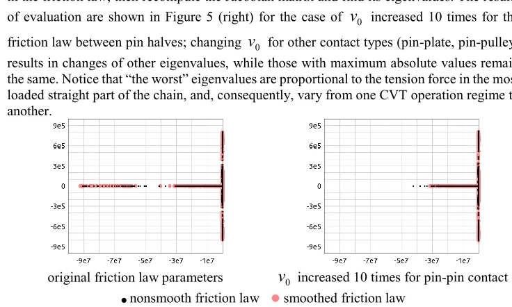
To make the search for an appropriate numerical method more purposeful, we have numerically solved the full eigenvalue problem at some typical state in a stationary regime of CVT operation. The eigenvalues found split into two groups: firstly, there are complex eigenvalues corresponding to damped oscillations; secondly, there are real negative eigenvalues corresponding to non-oscillatory dissipation processes. Absolute values of eigenvalue imaginary parts have maximum at approx.
10
6 s1 , while absolute values of real parts — at approx.10
8 s1. Figure 5 (left) shows the computed eigenvalues of the Jacobian matrix.Further we proved that the largest negative eigenvalues are caused by friction forces acting between pin halves, and the operating points in the friction law are at the linear part (
0
<
v
,
,
1,
=
,
~
=
Q
k
n
q
L
q
L
dt
d
k k k
(1)where
t
is the time,q
k are generalized coordinates,L
is the Lagrange’s function,Q
~
k are non-potential applied generalized forces, andn
is the number of degrees of freedom. Equations of motion can be rewritten in the normal form:
q
Q
A
v
L
t
v
q
P
P
A
v
F
v
q
x
x
t
F
x
=
(
,
),
=
,
=
1,
(
,
,
)
~
(2)(we took into account that the system is scleronomous), where
q
=
[
q
1,
,
q
n]
T is the vector of generalized coordinates,A
(
q
)
— symmetric positive-definite matrix of inertiawith elements
j i ij
q
L
q
A
2=
,v
— vector of generalized speeds,P
(
q
,
v
,
t
)
— essentiallynonlinear function, in particular due to
Q
~
containing friction forces.3 Investigation of numerical methods
Production versions of the CVT simulation software have been using the classical Runge –
Kutta numerical integration scheme of fourth order (RK4) [3] to solve the initial value problem of CVT dynamics. It is known that the RK4 scheme, as well as other explicit numerical integration schemes, have a step size limitation due to the stability requirement: in general, the value
h
, whereh
is the step size and
is an eigenvalue of ODE right-hand side Jacobian matrix, must belong to the stability region of the method.Due to that limitation, step sizes that can be used with RK4 vary in the range [
10
8 s, 710
s], which leads to long CPU time required for a simulation. In next subsection we analyze ODE system Jacobian matrix and explain the origin of its high eigenvalues. Then we proceed with the investigation of a number of numerical integration methods in application to CVT dynamics equations (2). The goal of the investigation is to find a method allowing much longer step sizes than RK4 and having the potential to run significantly faster than RK4.
3.1 Eigenvalues of ODE right hand side Jacobian matrix
To make the search for an appropriate numerical method more purposeful, we have numerically solved the full eigenvalue problem at some typical state in a stationary regime of CVT operation. The eigenvalues found split into two groups: firstly, there are complex eigenvalues corresponding to damped oscillations; secondly, there are real negative eigenvalues corresponding to non-oscillatory dissipation processes. Absolute values of eigenvalue imaginary parts have maximum at approx.
10
6 s1 , while absolute values of real parts — at approx.10
8 s1. Figure 5 (left) shows the computed eigenvalues of the Jacobian matrix.Further we proved that the largest negative eigenvalues are caused by friction forces acting between pin halves, and the operating points in the friction law are at the linear part (
0
<
v
v
). The idea of the proof is to change (e.g., increase 10 times) the saturation speedv
0in the friction law, then recompute the Jacobian matrix and find its eigenvalues. The results of evaluation are shown in Figure 5 (right) for the case of
v
0 increased 10 times for thefriction law between pin halves; changing
v
0 for other contact types (pin-plate, pin-pulley) results in changes of other eigenvalues, while those with maximum absolute values remainthe same. Notice that “the worst” eigenvalues are proportional to the tension force in the most
loaded straight part of the chain, and, consequently, vary from one CVT operation regime to another.
original friction law parameters
v
0 increased 10 times for pin-pin contactnonsmooth friction law smoothed friction law
Figure 5. Eigenvalues of ODE right hand side Jacobian matrix.
3.2 Numerical experiment setup
For each numerical integration scheme, two tests have been done. In the first test, the dependency of step local error norm
e
on the step sizeh
is investigated. The error iscomputed simply by comparison with the “exact” reference solution obtained with a very
small step size of
2
10
9 s using the RK4 scheme. In the second test, a dynamics simulation is performed during 0.005 second of real time; a sample history curve is obtained (namely, the axial force in a pin half entering a pulley set,P
z(
t
)
at certain pin — Figure 6) as an evident indicator of the acceptability of numerical results. Relative global errorE
of a numerical solution is estimated as|,
)
(
|
max
/
|
)
(
)
(
|
max
* ] ,0.005 * [ * ] s 0.005 , *[
P
t
P
t
P
t
E
z s t t z z tt
(3)where
P
*(
t
)
z is the reference curve;
t
*=
0.001
s has been chosen to avoid culling out somenumerical solutions due to a small time shift resulting in a large error at
t
[0,
t
*]
, which is not representative because the reference curve has a large slope at some pints in the range]
[0,
t
* . [image:5.482.52.420.77.298.2]nonsmooth smooth
Figure 6. Pin axial force history (reference curve).
)
(
*
t
P
znonsmooth smooth
Figure 7. Step local error for explicit methods.
To illustrate the impact of the nonsmoothness of friction law on the accuracy of numerical results, we included numerical results for two modifications of the model, differing only by the friction law (nonsmooth and smoothed, see Fig. 4, left and right respectively).
3.3 Explicit methods
Explicit methods covered in this subsection are the following classical ones.
Three embedded Dormand – Prince schemes with step size control [3]. The step size control was disabled in test simulations. An embedded scheme provides two solutions of different orders of accuracy at each step, which can be used to control the step size; those orders are encoded in the name of the scheme. The three schemes are DOPRI45 (orders 4, 5), DOPRI56 (orders 5, 6), and DOPRI78 (orders 7,8).
Gragg – Bulirsch – Stoer method with (GBS
p
s) or without (GBSp
) smoothing step [3]. It is an extrapolation method with the symmetric Gragg’s scheme used asthe reference scheme. We tried this method with a fixed extrapolation order
p
(2, 4, 6) and the harmonic step size sequence. Extrapolated explicit Euler scheme, with
p
extrapolation stages and the harmonic step size sequence (referred to as EULER-Xp
below).nonsmooth smooth
Figure 8. Global error for sample curve, explicit methods.
h
E
E
h
h
h
[image:6.482.71.424.330.642.2]nonsmooth smooth
Figure 7. Step local error for explicit methods.
To illustrate the impact of the nonsmoothness of friction law on the accuracy of numerical results, we included numerical results for two modifications of the model, differing only by the friction law (nonsmooth and smoothed, see Fig. 4, left and right respectively).
3.3 Explicit methods
Explicit methods covered in this subsection are the following classical ones.
Three embedded Dormand – Prince schemes with step size control [3]. The step size control was disabled in test simulations. An embedded scheme provides two solutions of different orders of accuracy at each step, which can be used to control the step size; those orders are encoded in the name of the scheme. The three schemes are DOPRI45 (orders 4, 5), DOPRI56 (orders 5, 6), and DOPRI78 (orders 7,8).
Gragg – Bulirsch – Stoer method with (GBS
p
s) or without (GBSp
) smoothing step [3]. It is an extrapolation method with the symmetric Gragg’s scheme used asthe reference scheme. We tried this method with a fixed extrapolation order
p
(2, 4, 6) and the harmonic step size sequence. Extrapolated explicit Euler scheme, with
p
extrapolation stages and the harmonic step size sequence (referred to as EULER-Xp
below). [image:7.482.62.422.436.633.2]nonsmooth smooth
Figure 8. Global error for sample curve, explicit methods.
h
E
E
h
h
h
e
e
The step local error test (Figure 7) shows that the local error is generally less for smooth friction law; further data processing also indicates that the local error behaves according to scheme order only in a limited step size ranges, different for different schemes; some schemes (DOPRI45, DOPRI78, GBS4, GBS6) do not show the expected behavior at all, although they do so in tests with simple ODEs.Global error in the dynamics test (Figure 8) confirms that all explicit schemes considered have severe step size limitation that is about
10
7 for nonsmooth friction law and schemes GBS2, DOPRI56, and is less for other schemes; for smooth friction law, the limit is higher yet it is less than5
10
7. We can also conclude that low order schemes (2–4) are preferable in model with both smooth and nonsmooth friction low; although some higher order schemes (e.g. GBS6s) give less error in model with smooth friction law, they are not an appropriate choice due to their complexity.3.4 Linearly implicit methods
There was a hope that a W-method [5] is capable of producing acceptable numerical solution at steps much greater than
10
7, because those methods generally have better stability properties than explicit ones. However, in our case all W-methods tested failed for some reason, though they worked good in tests with simple ODEs.The schemes considered in this subsection are SW24-
d
[5] (whered
is a parameter) and the W1 method extrapolated according to the Richardson’s procedure [3]. The W1 scheme isas follows:
),
(
)
,
(
=
11 k k k k k
k
x
hF
t
x
hdA
x
x
x
(4)where
x
is the numerical solution vector, the subscriptk
denotes the step number,h
is the step size,t
is the time,F
is the ODE right-hand side vector,d
is a parameter (usually between 0 and 1), andA
is a matrix approximating the ODE system JacobianDF
/
Dx
. W-methods are attractive compared to Rosenbrock W-methods [6] due to the ability to keepA
constant during many time steps, thus eliminating the necessity to compute it and factorize the matrix
I
hdA
at each time step. Schemes resulting fromp
extrapolation stages of W1 are further referred to as W1-Xp
-d
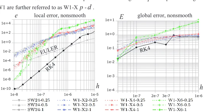
.local error, nonsmooth global error, nonsmooth
Figure 9. Local step error and global error for sample curve, linearly implicit methods compared to RK4 and explicit Euler methods.
e
E
Figure 9 (left) shows that all schemes tested have much greater local step error than explicit schemes. The expected order of schemes is observed at step sizes less than
10
7; the higher the order, the narrower the range in which scheme order is obeyed. Figure 9 (right) shows that all W-method schemes produce inacceptable solution (E
>
0.05
) even at step10
7.We have to conclude that they didn’t work in our case.
3.5 Trapezoidal Rule Method
Among many implicit methods, we chose the trapezoidal rule (a 2-nd order scheme), further abbreviated as TRPZ:
)],
,
(
)
,
(
[
2
=
11
k
k k
k
kk
x
h
F
t
x
F
t
h
x
x
(5)Figure 10 shows the step local error for the trapezoidal rule. Notice that it is less than for any other scheme tested at steps greater than
4
10
7.Sample curves obtained at step size
2
10
6 practically coincide with reference curves; global errorE
is1.4
10
3 for nonsmooth friction law and5.6
10
4 for smooth frictionlaw. It is possible to use larger step sizes, but only with step size control because the Newton’s
[image:8.482.66.419.326.450.2]method used at a time step may fail to converge.
Figure 10. Step local error for trapezoidal rule, compared to RK4 and explicit Euler methods. Notice that, despite the large step size in the trapezoidal rule method, it does not currently run faster than RK4. The reasons are the necessity to solve a system of nonlinear algebraic equations at each step using an iterative Newton-like method, and the need to compute the
Jacobian matrix. We omit details here, but in short, the number of Newton’s iterations is low
(2–3) when the Jacobian matrix is recomputed at each iteration, and is significantly higher (10–20) in cases with approximated Jacobian matrix (e.g., using an update formula similar to
the Broyden’s one [7]).
3.6 Stabilized explicit method
Having investigated the stiffness properties of the ODE system, we decided to consider so called stabilized explicit, or Chebyshev – Runge – Kutta [8, ch. IV.2], numerical integration methods. Among those we picked the one called DUMKA3 [9]. The choice of that particular method was based on public availability of solver implementation code in C programming language.
e
Figure 9 (left) shows that all schemes tested have much greater local step error than explicit schemes. The expected order of schemes is observed at step sizes less than
10
7; the higherthe order, the narrower the range in which scheme order is obeyed. Figure 9 (right) shows that all W-method schemes produce inacceptable solution (
E
>
0.05
) even at step10
7.We have to conclude that they didn’t work in our case.
3.5 Trapezoidal Rule Method
Among many implicit methods, we chose the trapezoidal rule (a 2-nd order scheme), further abbreviated as TRPZ:
)],
,
(
)
,
(
[
2
=
11
k
k k
k
kk
x
h
F
t
x
F
t
h
x
x
(5)Figure 10 shows the step local error for the trapezoidal rule. Notice that it is less than for any other scheme tested at steps greater than
4
10
7.Sample curves obtained at step size
2
10
6 practically coincide with reference curves; global errorE
is1.4
10
3 for nonsmooth friction law and5.6
10
4 for smooth frictionlaw. It is possible to use larger step sizes, but only with step size control because the Newton’s
[image:9.482.79.409.314.462.2]method used at a time step may fail to converge.
Figure 10. Step local error for trapezoidal rule, compared to RK4 and explicit Euler methods. Notice that, despite the large step size in the trapezoidal rule method, it does not currently run faster than RK4. The reasons are the necessity to solve a system of nonlinear algebraic equations at each step using an iterative Newton-like method, and the need to compute the
Jacobian matrix. We omit details here, but in short, the number of Newton’s iterations is low
(2–3) when the Jacobian matrix is recomputed at each iteration, and is significantly higher (10–20) in cases with approximated Jacobian matrix (e.g., using an update formula similar to
the Broyden’s one [7]).
3.6 Stabilized explicit method
Having investigated the stiffness properties of the ODE system, we decided to consider so called stabilized explicit, or Chebyshev – Runge – Kutta [8, ch. IV.2], numerical integration methods. Among those we picked the one called DUMKA3 [9]. The choice of that particular method was based on public availability of solver implementation code in C programming language.
e
h
A stabilized explicit scheme has stability region, defined by the condition
|
R
s(
h
)
|
1
, extended into real negative direction of complex planeh
. The functionR
s is a polynomial of degrees
, called the stability polynomial.The DUMKA3 solver actually implements a family of
s
-stage Runge–Kutta schemes, each of which realizes stability polynomial of degrees
varying from 3 up to 324. The solver implements automatic step size control, based on step local error estimation, and polynomial degree control, based on the estimation of ODE right hand side Jacobian matrix spectral radius. Preliminary tests have shown that solver performance with both control options enabled is far from optimal in our system. Besides, numerical estimation of Jacobian spectral radius don’t work well due to discontinuities of the ODE right hand side in the case ofnonsmooth friction law, resulting sometimes in too large values. We disabled both control options. The motivation was to obtain best performance at fixed step for each fixed polynomial degree. Giving each polynomial an index
k
from 0 to 13 (DUMKA3 implements 14 polynomials), we denote corresponding schemes by suffixes -Pk
. In particular, we tested degreess
=
21
(k
=
4
),s
=
27
(k
=
5
),s
=
36
(k
=
6
),s
=
48
(k
=
7
),s
=
63
(8
=
k
),s
=
81
(k
=
9
). Polynomialsk
4
andk
9
have shown poor performance: in the first case the stability region is too small in the real negative direction, and in the second case it is too small in the imaginary direction.local error, nonsmooth global error, smooth
Figure 11. Local step error and global error for sample curve for DUMKA3, compared to RK4 and explicit Euler methods.
Figure 11 (left) shows the dependency of step local error norm on the step size. DUMKA3 results are compared against RK4 and the trapezoidal rule; the latter one is known (see sec. 3.5) to give sufficiently accurate solution at
h
=
2
10
6 s. It can be shown that the slope for each curve at steps below10
6 corresponds to the order of the scheme (3 for DUMKA3, 4 for RK4, and 2 for TRPZ). Notice also that at steps above10
6 local error for all DUMKA schemes rises sharply at some point; additional error jumps can be seen at step10
6 for nonsmooth friction law. At large step sizes, local error for DUMKA schemes is approximately the same as for the trapezoidal rule, in the case of smoothed friction law; for nonsmooth fricion law, the trapezoidal rule gives smaller error.Figure 11 (right) shows the global error for sample curve. It follows from the figure that schemes DUMKA3-P5 – DUMKA3-P8 give sufficiently accurate solution at step
6
10
2
=
h
, and at steph
=
4
10
6 only the scheme DUMKA3-P8 does so.e
E
Table 1. Performance of DUMKA3 schemes compared against RK4.
scheme
h
, sn
RHS speedup againstRK4
RK4
5
10
8 400824 1DUMKA-P5
2
10
6 75817 5.9DUMKA-P7
3
10
6 95425 4.7DUMKA-P8
4
10
6 104821 4.4Comparing simulation times, we can conclude that the DUMKA3 solver can perform simulations several times faster than RK4, which is summarized in Table 1. Notice that the value
n
RHS in the table is the total number of ODE right hand side evaluations in the test simulation (the one used to obtain the sample curve).4 Conclusions and Future Work
This paper represents the results of an investigation of application of different numerical integration methods to the ODEs of CVT dynamics model, in a hope to find a potentially faster method. The investigation has shown that traditional explicit numerical integration schemes and W-methods don’t work in our case. Implicit methods give good results; however, to make those methods run faster than RK4, additional efforts are required: for example, ODE right-hand side Jacobian could be computed much faster but it requires tedious programming (the idea is to combine the approach presented in [10] with the decomposition of the ODE right-hand side into a sum and providing faster code for the Jacobian of contact forces). The attempt to use stabilized explicit Runge – Kutta solver, RK4, has proven to be successful in terms of performance. However, the original polynomial order
control implemented in the solver doesn’t work: it tends to increase polynomial order, but in
that case Jacobian eigenvalues with maximum imaginary parts fall outside the stability region. This motivates us to consider other stabilized explicit solvers, first of all RKC and SERK2 [11], and probably others, constructed according to the approach presented in [12], because there is a way to construct a method with stability region that best fits the spectrum of ODE right hand side Jacobian.
References
1. N. Shabrov, Yu. Ispolov, S. Orlov, ZAMM 94(11) (2014) 2. S. Orlov, A. Kuzin, N. Shabrov, CCIS 793 (2017)
3. E. Hairer, S. Nørsett, G. Wanner, Solving Ordinary Differential Equations I: Nonstiff Problems (Springer-Verlag, New York, 1993)
4. K. Johnson, Contact mechanics (Cambridge University Press, Cambridge, 1987) 5. T. Steihaug, A. Wolfbrandt, Math. Comp. 33(146) (1979)
6. H. Rosenbrock, Comput. J. 5 (1963) 7. C. Broyden, Math Comp. 19 (1965)
8. E. Hairer, G. Wanner, Solving Ordinary Differential Equations II: Stiff and Differential-Algebraic Problems (Springer-Verlag, Berlin Heidelberg, 1996)
9. Medovikov, BIT Numerical Mathematics 38(2) (1998) 10. T. Ypma, J. Comput. Appl. Math., 18(1) (1987)