University of Southern Queensland
Faculty of Engineering & Surveying
Real Time Implementation of Obstacle
Avoidance for an Autonomous Mobile Robot
Using Monocular Computer Vision
A dissertation submitted by
Iain Brookshaw
in fulfilment of the requirements of
ENG4112, Research Project
towards the degree of
Bachelor of Mechatronic Engineering
Abstract
For autonomous robotic motion, it is essential for the mobile machine to be able to judge its position relative to potential obstacles. This implies the ability to identify potential obstacles, study their approach and take appropriate action when necessary to avoid collision. In this age of cheap and available digital cameras and powerful computers, it is desirable to achieve this with a single digital camera as the sensor.
The digital camera has the advantages that it is cheap, easily installed, well understood, passive and physically small. When coupled with a small, powerful on-board computer it has the potential to create a effective obstacle avoidance system.
This investigation was attempt to create just such a system. A series of methods dealing with identifying, tracking and avoiding obstacles were be investigated, and the results of their implementation discussed. Alternative methods were be analysed and weighed. It was the initial intention to produce a program that could identify parts of the image as “obstacles”, determine the approach of these obstacles and use this information to direct a small mobile, autonomous machine.
the final result was too inconsistent to enable true avoidance to be implemented.
The inconsistencies in the results were largely due to small errors in each section compounding as the program evolved. However, a wide range of tests on each of the component parts of the system illustrated that the concepts and methods selected are viable individually. While there were problems with consistency when the program is run, it was clear from the results that the individual components could be made to function if additional time was spent correcting errors.
University of Southern Queensland
Faculty of Engineering and Surveying
ENG4111/2
Research Project
Limitations of Use
The Council of the University of Southern Queensland, its Faculty of Engineering and Surveying, and the staff of the University of Southern Queensland, do not accept any responsibility for the truth, accuracy or completeness of material contained within or associated with this dissertation.
Persons using all or any part of this material do so at their own risk, and not at the risk of the Council of the University of Southern Queensland, its Faculty of Engineering and Surveying or the staff of the University of Southern Queensland.
This dissertation reports an educational exercise and has no purpose or validity beyond this exercise. The sole purpose of the course pair entitled “Research Project” is to contribute to the overall education within the student’s chosen degree program. This document, the associated hardware, software, drawings, and other material set out in the associated appendices should not be used for any other purpose: if they are so used, it is entirely at the risk of the user.
Prof F Bullen
Dean
I certify that the ideas, designs and experimental work, results, analyses and conclusions set out in this dissertation are entirely my own effort, except where otherwise indicated and acknowledged.
I further certify that the work is original and has not been previously submitted for assessment in any other course or institution, except where specifically stated.
Iain Brookshaw
0050086292
Signature
Acknowledgments
This thesis was typeset using the LATEX 2ε typesetting program.
The author would like to thank Dr. Tobias Low for his clear guidance, Dr. Leigh Brookshaw, for his generous assistance, Mr. Erin Heaton for his longstanding support and finally, all those poor souls who showed great patience whilst the author excitedly showed off the latest results.
Iain Brookshaw
Contents
Abstract i
Acknowledgments v
List of Figures xiii
Chapter 1 Introduction 1
1.1 Computer Vision and Mobile Robots . . . 3
1.2 Objectives . . . 3
1.3 Background, Vision and Image Processing . . . 4
1.3.1 Image Acquisition and Processing . . . 4
1.3.2 Software and Libraries . . . 5
1.3.3 Hardware Preconceptions . . . 6
1.4 Chapter Summaries . . . 7
2.1 Why Segment an Image? . . . 11
2.2 Segmentation Methods . . . 13
2.2.1 Thresholding . . . 13
2.2.2 Edge Detection . . . 14
2.2.3 Region Growing . . . 18
2.2.4 Split and Merge Techniques . . . 20
2.3 Single Pass Split Merge Segmentation . . . 21
2.3.1 Merging Algorithm . . . 22
2.3.2 Splitting Algorithm . . . 24
2.4 Image Pre-Processing . . . 31
2.4.1 Noise Removal and Image Smoothing . . . 31
2.4.2 Finding a Tolerance . . . 32
2.5 Potential Problems . . . 34
Chapter 3 Distance and Approach 35 3.1 Methods of Distance Estimation . . . 38
3.2 Looming . . . 41
3.2.1 Area . . . 42
CONTENTS ix
3.2.3 Texture . . . 45
3.2.4 Blur . . . 46
3.3 Implementation . . . 52
3.3.1 Blur Calculation . . . 52
3.3.2 Looming Calculation . . . 55
3.4 Avoidance . . . 56
3.4.1 Approach Categorisation . . . 56
3.4.2 Direction Decisions . . . 57
Chapter 4 Tracking and Correlation 59 4.1 Frame to Frame Correlation . . . 61
4.2 Point or Feature Tracking . . . 62
4.3 Region Tracking . . . 64
4.4 Chosen Algorithm . . . 65
4.4.1 Centroid Calculation . . . 66
4.4.2 Data Recording . . . 69
4.4.3 Centroid Matching . . . 70
5.2 Segmentation Verification . . . 76
5.2.1 Effects of Pre-Processing Filtering . . . 78
5.3 Centroid Verification . . . 80
5.4 Tracking Testing . . . 81
5.5 Blur Estimation . . . 84
5.6 Looming Computation . . . 93
5.6.1 Area Looming . . . 93
5.6.2 Blur Looming . . . 95
5.7 Discussion . . . 96
5.7.1 Segmentation . . . 96
5.7.2 Tracking . . . 97
5.7.3 Looming . . . 99
Chapter 6 Conclusions 103 6.1 Segmentation . . . 105
6.2 Tracking . . . 105
6.3 Looming . . . 106
6.4 Overview . . . 106
CONTENTS xi
Chapter 7 Future Work 109
7.1 Obstacle Detection . . . 111
7.2 Tracking and Correspondence . . . 112
7.3 Looming, Approach and Avoidance . . . 113
7.4 Navigation . . . 115
References 117 Appendix A Original Specifications 121 A.1 Research Specification . . . 123
Appendix B Program Listings 125 B.1 Final Programs . . . 127
B.1.1 Main Driver Function . . . 127
B.1.2 Segmentation Functions . . . 131
B.1.3 Centroid Finding Functions . . . 146
B.1.4 Tracking Function . . . 153
B.1.5 Looming Function . . . 157
B.2 Testing Algorithms . . . 158
B.2.1 Segmentation Test Program . . . 158
List of Figures
2.1 Illustration of the pixels in an image. Counter clockwise from top: the original image, a close up illustrating the graduations of pixels and a extreme close up, illustrating the graduation of pixels in an object. . . 12
2.2 Illustration the single pass split and merge operation, showing the four pixel group and the previously labeled pixels. . . 20
2.3 The merging algorithm as implemented . . . 23
2.4 The orientation of the pixels in the four pixel block. This orienta-tion is also used in the final program . . . 24
2.5 The original splitting algorithm, which was not implemented suc-cessfully . . . 25
2.6 The various combinations possible with a four by four pixel block. Note thatviii and ix are the same. . . 28
2.7 The final splitting algorithm, where splitting was based on patterns in order of precedence . . . 31
3.2 Stereo vision, using one camera and the frame difference to find depth. . . 38
3.3 Graphical depiction of Looming using projected area. . . 41
3.4 The Gaussian curve, showing standard deviation (σ) and the true radius of blur . . . 47
3.5 Plot of various step functions representing the region edge with varying degrees of ideal blur. f(x) is the original step, with b(x) being the camera’s blurred edge and ba(x) and bb(x) being the re-blurred edges. . . 48
3.6 Plot of Rmax values recovered in Note the symmetrical nature of the plot around the region boundary. . . 49
3.7 Illustration of finding the four points of a region for blur compu-tation. The left hand image shows the case of the centroid being in the region. The right hand image is for the centroid being out of the region. . . 54
4.1 Illustration of the difficulties of tracking for non-orthogonal move-ment . . . 63
4.2 the recursion algorithm as used by the tracking program . . . 68
LIST OF FIGURES xv
5.2 Illustration of segmentation of a complex image. On the left, the original image, on the right the segmented output. n.b. this image was used as a test image in (Hu & de Haan 2006) (among others) and was repeated as a test image here as the author found its prove-nance rather amusing. In actuality any reasonably uncomplicated image would do. . . 78
5.3 Illustration of the differences between two segmented images. The top set is 2% smaller than the bottom set. Notice the region dis-crepancies, especially in the foreground. . . 79
5.4 The test image, showing the successful finding of the centroids. . . 81
5.5 The test more complex test image image, again showing the suc-cessful finding of the centroids. . . 81
5.6 Checkerboard test image distorted for tracking. 600 by 600 pixels 82
5.7 Distorted checkerboard showing tracked centroids. The grey line from the centroids in the right hand figure shows the computed position of the centroids in the previous (left hand) frame. . . 82
5.8 The results of tracking the segmented images in figure 5.3. The line from each centroid indicates the calculated position of that region in the previous frame. . . 85
5.9 The ideal blur test image. It is simply a two square checkerboard 400 by 200 pixels. Note the grey values used to colour the squares are not black and white. . . 85
5.11 The step functions for the blurred edges showing the initial recov-ered blur and the two re-blurred edges. Re-blur σ values of 4 and 7. . . 90
5.12 Maximum recovered blur difference for the ideal test image with initial radius of 1 and a re-blurσ values of 4 and 7. . . 91
5.13 Multi-coloured test image for general blur recovery tests. . . 92
Chapter 1
1.1 Computer Vision and Mobile Robots 3
1.1
Computer Vision and Mobile Robots
Giving functioning robots the ability to “see” and understand their environment through complex anthropomorphic optical sensors is a long sought after goal in robotics. Such sensors have the distinct advantage of being passive (in that they do not give off any signal, they simply receive data) and are able to obtain much information about their environment from relatively simple sources. Currently, with the development of sophisticated, inexpensive web cams such systems are practicable for minimal cost.
In order to implement a system that can use such vision to avoid obstacles, much information must be recovered from the digital image. The information that a human obtains without conscious effort (relative size of objects, their position and their very extent) must be laboriously recovered from the image data. What follows is chiefly concerned with recovering information that could then be used to guide a hypothetical autonomous machine.
The critical information for the avoidance of obstacles is: the extent of objects in the image, their correspondence to objects in previous images and their position relative to the viewer. This is fairly obvious and the reader can do all of these things without effort, however it can be a laborious process to recover these things from the image flow. Thus the minimal form of any machine attempting to navigate via vision is a camera, a computer (of significant processing speed) and a mechanism for controlling the drive.
1.2
Objectives
The final programs were intended to separate an object from its surroundings, make an estimate of its approach and use this data to formulate a response for the machine. This was meant to be implemented with only one camera.
Time permitting, these were intended to be extended to include true navigation, as opposed to simple avoidance.
In the event, these were found to be overly simplistic objectives. Other unforeseen problems extended the project in some directions and curtailed it in others. For a detailed list of initial specifications see Appendix A.1.
1.3
Background, Vision and Image Processing
1.3.1
Image Acquisition and Processing
Machine vision has a great many meanings and applications. All, to some degree, revolve around interpreting the response of photo-sensitive electronics to changing light conditions. In this case a simple web-cam type digital camera was used to obtain a detailed picture of the immediate surroundings. It was intended at all stages of the project that the final results would be obtained from inexpensive cameras of this sort.
Once the image has been obtained from the camera, a variety of filters and algorithms were applied to obtain information, such as object location, position and approach. All of these filters involved running over the image (frequently pixel by pixel) and recording data.
A digital image, the output of the camera, is simply an array of numbers con-taining the values for brightness at that point, as interpreted by the camera. 1
1The basics of a digital image can be obtained from any text on the subject. The information
1.3 Background, Vision and Image Processing 5
Add enough elements to this matrix and an image of recognisable complexity is created. This image could be colour or gray-scale. In the former, the matrix is three dimensional with several values or channels (usually Red, Green, Blue and alpha or transparency) for each pixel or point in the image. It is the combination of these values that comprises the “colours” one sees. By contrast the latter ar-rangement has only one number per pixel, a integer of value 0 to 255 (in a colour image data is also stored in integers in this range). This means that there is only shadings of light to dark for each pixel (usually 255 is fully white and 0 is fully black). The reason for this range is that it enables one byte, 8 bits to be used for every pixel (28 = 256, hence 256 is the maximum integer that can be stored in an 8 byte space). For simplicity, single channel gray-scale images were used throughout this project. It was not felt that colour would give any noticeable advantage.
The key point from all this description, is that the image fundamentally remains an array of integer points from 0 to 255, and as such can be treated with numerical approaches like any other array of data.
1.3.2
Software and Libraries
To implement any algorithm in the computer vision field it is necessary to first select the programming environment. In this case the selection was governed by two key constraints, speed and ease of use. As the focus was real time applications, the program execution must be rapid in the extreme. This immediately ruled out scripting languages such as Matlab(although Matlab was used in very early
stages as a familiar environment in which to test ideas, the code developed was very limited and is not included). Furthermore, the programing language needed to be simple to learn and debug, with a wide range of support and documentation (when the project began the author had familiarity withMatlabonly) as it was
anticipated that no time could be spared for programing errors brought on by ignorance.
Considering these factors and soliciting advice from several parties, finally led to the selection of C as the programing language and the Open Computer Vi-sion library as the basis for further programing. The existence of a open source computer vision library (recommended by Dr. Tobias Low) was critical in this decision.
All programs developed throughout this project use this library as a basis and rely on it for frame acquisition, image format and data storage and low level manipulation. The complete library can be obtained fromhttp://sourceforge. net/projects/opencvlibrary.
All code was compiled on a Debian Linux machine (version 6.0.3) using the gcc compiler (version 4.4.5) linked with the OpenCV library (version 2.1).
1.3.3
Hardware Preconceptions
Mobile robots and autonomous machines are the objectives of many fields of study. While the applications are obvious, there are a great number of them and the methods used to develop solutions to one may not necessarily apply to the others. Throughout this project the focus has been on developing a vision system for a small scale autonomous device. The resultant designs may not function out of this context.
1.4 Chapter Summaries 7
addition it was assumed that the objects in view would all be rigid and static. Thus the initial vision for the end user was a small machine operating indoors in an environment where the only movement in the image was caused by the camera’s motion.
The reasons for these limitations were simple. Although the focus called for “real time” initial research quickly showed that any method would involve a good deal of image manipulation. This was expected to slow computation considerably. Thus the speed of the machine (and hence the discrepancy between frame) should be reduced. As this implied a slow moving device, the other assumptions soon followed.
As it transpired the programs were never implemented on actual hardware (time being prohibitive and results limited). Nevertheless, the above considerations formed the background to all stages of the project
1.4
Chapter Summaries
• Chapter 2 covers the ways and means of separating objects from their sur-roundings. A number of processes are reviewed and the final method eluci-dated.
• Chapter 3 discusses ways of quantifying the approach of these objects. While a number of methods were reviewed, the Looming approach was finally decided upon.
• Chapter 4 describes how frame to frame correlation of objects was accom-plished.
• Chapter 5 covers the results of implementation.
Chapter 2
Image Segmentation and Obstacle
2.1 Why Segment an Image? 11
2.1
Why Segment an Image?
When instructing a computer to avoid obstacles, the first difficulty is defining what is meant by an “obstacle”. When a person examines a scene, they are capable of separating one object from another. Intuitively a person knows that this object is here, it is occluded by this object, which is obscured by this object and so on. Many people are probably wholly unaware of what they are doing when they make these distinctions. Electronic eyes have no innate ability to create these distinctions. The computer does not “see” anything, per say, instead the light is detected and transformed into a matrix of numbers, representing the colour and intensity of the light at that discrete point or pixel.
This matrix is the computer’s representation of an image. The light and dark pat-terns, which the human eye and mind would instantly recognise as a representa-tion of three dimensional space, mean nothing to the computer (Jain et al. 1995)). This is a critically important point and one that must be held in constantly mind. While the image may represent familiar objects to the viewer, to the computer they are only numbers in an array. Furthermore, these numbers represent the projection of the three-dimensional space on a two-dimensional plane. Thus it follows that the computer is incapable of recognising one object from another, or even distinguishing between foreground and background without aid.
This would appear to be fairly obvious, yet it is easy to confuse the image as the eye sees it and the image as the computer interprets it. Segmentation is the first step in enabling the computer to differentiate between objects. More succinctly, segmentation is “to divide an image into parts that have a strong correlation to objects or areas of the real world” (Sonka et al. 1994) pg 112). A close examination of a digital image will reveal that a single object is not represented by pixels of a single colour (see figure 2.1). Instead, an object is represented by pixels of graduated intensity1. This represents the shading caused
Figure 2.1: Illustration of the pixels in an image. Counter clockwise from top: the
original image, a close up illustrating the graduations of pixels and a extreme close
up, illustrating the graduation of pixels in an object.
by the reflection of light from the surface. Notice that while there may be a clear edge (see section 2.2.2) the pixel values within this edge (the object boundary) may all be different.
Segmentation, then is the means by which all pixels within an object are dis-tinguished from the pixels in another object (Sonka et al. 1994). This can be done several ways, but its purpose is to enable subsequent routines to distinguish between one obstacle and another, assign values of range and depth (see section 3.1) and conduct avoidance and navigation calculations. This can only be done swiftly if each object in view is clearly distinguishable from all others.
2.2 Segmentation Methods 13
2.2
Segmentation Methods
There are a number of ways of splitting an image into it’s component parts. All to some extent rely on the change in some numeric property at the object boundary, or similarity of connected pixels that represent an object (Jain et al. 1995). The various approaches most commonly described in the relevant literature include: Thresholding, Edge Detection and Split-Merge techniques . In this particular project, a species of the split merge technique was selected.
2.2.1
Thresholding
Although too simple for the purposes of this project, the Thresholding method provides a good illustration of many of the techniques used in more applicable methods.
Essentially, the Thresholding method is based separating an object from its back-ground (Sonka et al. 1994). A threshold is selected based on analysis of the image properties (Jain et al. 1995) and each pixel compared to this value. The pixels in the output image are then assigned as 255 or 0 depending on which side of the threshold the input pixel falls.
Relying on a clear distinction between objects and background, this method is usually divides the image into two segments, background and foreground. A more complex version of this is band Thresholding, described in (Sonka et al. 1994). In this approach, bands of grey-scales are selected and the pixels sorted into these bands. In essence it is the same technique, but using several thresholds instead of one. This is a useful method for objects of known grey-levels (Sonka et al. 1994).
obscure edges and indeterminate outlines. Additionally, the assumption that there is two or a small limited number of arbitrary regions is clearly too crude for obstacle avoidance in an unknown environment. However, the Thresholding method illustrates the basic idea that like pixels are arranged into groups and that this likeness is judged by the numerical value of each pixel. Furthermore, the concept of a threshold is an important one. Most segmentation methods employ some means of establishing demarcation, some numerical value acquired from analysis of the entire image data that establishes a boundary.
2.2.2
Edge Detection
A much more sophisticated method than Thresholding, edge detection methods rely on the change in pixel values between objects. Requiring much less prior knowledge of the image (Sonka et al. 1994), edge detection is a potentially more powerful tool. However, in the context of obstacle avoidance it created a number of difficulties in application. Namely, the difficulty in creating closed outlines and problems related to objects that may not have edges (such as walls in close proximity). While the former may be overcome (see section 2.2.2), the latter poses a more complex problem. Although a useful tool, it was felt to possess more drawbacks and fewer advantages compared to the the chosen system (see section 2.3).
2.2 Segmentation Methods 15
edge detection were inherent in the result, rather than the process, these were not investigated in great detail. Suffice it to say that most edge detection relies on the assumption that there is some clear demarcation between the group of pixels representing one object and the pixels representing another (Sonka et al. 1994). It is frequently assumed that the this intensity changes takes the form of a step, ramp, impulse or similar function (in one dimension) (Jain et al. 1995). The result of this process is a series of unrelated “dots”, pixels that fit a criterion of an edge.
Once the edges have been established it is becomes necessary to produce contours, a list or mathematical curve that describes the edges (Jain et al. 1995). The validity of the edges must be assessed, their strength or weakness evaluated to remove weak edges (those with a low probability of existence, based on their surroundings (Sonka et al. 1994). Then the gaps in edges must be filled. Finally, one has to break the image into regions based on the results of this process (or use the contours themselves, see below). Each step in this process would require a unique pass of the image and all of these passes are simply those needed to create successful segmentation. It does not include the prepossessing steps. Such an involved process was felt to be too computationally intensive to employ.
It could be argued that once these contours have been established, one need only use the resultant edges to define obstacles, without further segmentation. This is partially true, however it causes problems not only with the method used to track and gauge distance 2 but causes problems with obstacles that are too large
to see.
Consider a wall, it is clearly an obstacle, yet unless its end is in view or it is heavily textured, it produces no edge, only a line on the floor. This line would not noticeably expand or contract as the camera approached, it would simply move 2see section 3.2 it could become difficult to establish the motion of a contour owing the
“up” and “down” the image frame. During the early stages of the project this was felt to be unsatisfactory from a Looming perspective (see section 3.2), owing to the fact that the line area was not expanding. Later when blur was selected this problem became less of an issue and the need to have two dimensional objects became less important. However, by that stage other segmentation methods were chosen.
Edge detection was investigated in the initial phases of the project and discarded when many of the methods outlined in sources returned only a disconnected series of dots. These “edges” could have to then be amalgamated into contours, that could then be used to create regions. This seemed a very time consuming and pain full process. Discouragement with uninspiring initial results involving the Canny Edge detection algorithm (Bradski & Kaehler 2008) reinforced this view. It was later discovered that there were far more effective means of employing edge detection methods (see section below).
Edge Tracing
Following the author’s decision to use region based segmentation (see below) as the basis of obstacle detection, an alternative method, Edge Tracing was sug-gested. Although a potentially highly applicable and useful tool, this method was not implemented due to time constraints, the completion of segmentation sections and other, contrary advice.
2.2 Segmentation Methods 17
(Billingsley 26th May 2011).
By contrast, an tracing algorithm, searches until an “edge” is found, then follows the edge by searching the surrounding pixels for the next stage. The next pixel in the line is then found and the program moves forward until no surrounding pixels meet the edge criteria. Thus from this process a continuous line is found, with a definite start and conclusion for each edge. This method can be made swifter by employing various search patterns on the basis of spirals to remove the necessity of searching every pixel in the image (Billingsley 26th May 2011).
While far more efficacious than any other edge detection method, the edge tracing algorithm was not selected for final use in the finished program for a number of reasons. When identified to the author, writing for the final segmentation algorithm (see below) was already nearing completion. It was initially felt that additional expenditure of time could not be justified, especially as virtually all existing work would have to be rewritten and for a method that was bound to have unforeseen and time consuming side issues. Secondly, it was believed that the edge based approach suffered from a serious flaw. By definition only the outlines of objects are considered. While this requires far less computational power than other methods (only a tiny fraction of the image is under consideration (Billingsley 26th May 2011), it renders most of the image a blank map with no information about those pixels. If the machine was to approach a blank wall, an edge detection device could only extract information about the line where the floor meets the wall.
knowing that the line representing the top is connected to the line representing the bottom. Thus a shallow “step” could be misinterpreted as an insurmountable obstacle. This and other similar objections lead to the belief that it would be far more useful if all the pixels representing the object could be labeled and the object’s full extent known.
Having full knowledge of an object’s extents could enable the final program to be expanded into other areas (eg: object recognition, identification etc.) and while such expansion was beyond the scope of this project, after consultation (Low 15/12/2010 to October 27/10/2011) it was agreed that Edges did not offer the best chances for future expansion and that a region based approach might be more efficacious.
2.2.3
Region Growing
Where edge detection can be used to outline a region for later segmentation, re-gion growing functions in the opposite direction. The rere-gions are defined directly, producing blocks of continuous colour that define the extent of an object. The resultant image can then be combined with edge detection methods if the edges are desired (Davies 1997). The methods for region growing are based around determining the similarity (or dissimilarity) of regions, on the assumption that all pixels that represent an object will exhibit similar characteristics.
2.2 Segmentation Methods 19
Merging Techniques
The merging technique is relatively self explanatory. Essentially, like regions are joined or merged as judged by some homogeneity criterion. This criterion is usually based on the grey-scale properties of the regions in question.
The simplest, but most expensive way of implementing this method (as described in (Sonka et al. 1994) is to consider every pixel as a separate region and try to merge a pixel with its neighbours. If the neighbours are “similar” then those pixels are marked by the same colour in the output image and the program moves on. Therefore for a image of n pixels by m pixels one begins with n×m separate regions and continues to merge adjacent regions into large segments until it is no longer possible to merge a new pixel without violating the predefined homogeneity criterion. Thus one grows regions much as one would grow a crystal in a jar and at about the same speed.
Needless to say, this is far to slow and simple a method to employ for a real time application. However, it does serve to illustrate the merging method.
Splitting Techniques
Virtually the exact algorithmic inverse of the pure merging method, region split-ting takes the entire image as one region and successively breaks it into smaller regions. The original full image region is broken down repeatedly until it is im-possible to segment further without violating the homogeneity criterion. When this point is reached it means that all the remaining regions satisfy the criterion and can be considered as a single object.
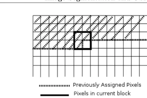
Figure 2.2: Illustration the single pass split and merge operation, showing the four
pixel group and the previously labeled pixels.
Once again, it is apparent that this method, by itself is unsatisfactory for the same reasons as above.
2.2.4
Split and Merge Techniques
The most promising method of image segmentation arose from the split and merge branch of techniques. As mentioned above they are not direct inversions, however when used in conjunction they may produce an efficient and effective algorithm (Sonka et al. 1994).
It is possible to combine the split and merge algorithms to produce a more sat-isfactory result. The simplest way to do this is to subdivide the image into a grid of four large regions (Yang & Lee 1997), then recombine two or more of the four if they meet some homogeneity criterion (usually the mean grey-scale value). The resulting regions are then split into four again (if this is possible without violating the criterion) and the process of combination repeated with the new sub-regions. This process is repeated until it is no longer possible to split the sub-regions without violating the criterion used (Sonka et al. 1994).
2.3 Single Pass Split Merge Segmentation 21
prospective region is measured and compared to a set tolerance (Davies 1997). Al-ternative approached include approximating the region to a planar surface (Yang & Lee 1997). If the mean squared error is below a certain tolerance the region is homogeneous.
Needless to say, this approach is almost as slow and computationally intensive as the previously mentioned split or merge methods. It is significant, however in illustrating the combination of the split and merge concepts. The idea of initial splitting and later re-merging can be adapted to give a much more rapid and successful method.
2.3
Single Pass Split Merge Segmentation
The basic split and merge technique, while easy to explain, somewhat compu-tationally expensive and slow (Sonka et al. 1994). This can be remedied by a conceptual modification referred to as Single Pass Split and Merge. This algo-rithm is capable of segmenting the image in one pass, rather than the complex tree structure described above. Due to the real-time focus of the project, this was eventually the method selected.
The method works in two distinct stages. First a small section of the image is subjected to a splitting algorithm and labels assigned to the pixels accordingly. These split pixels are then compared to the regions in the main image to which they were previously assigned and the split groups merged to their larger coun-terparts as appropriate. The similarity or dissimilarity of pixels and regions is determined by a tolerance established by the image properties (Sonka et al. 1994).
image where possible and new regions begun where not. This way the entire segmentation process is performed as the square advances. Other merging or splitting methods imply multiple levels of processing and multiple passes through the image (Dep 1998). See figure 2.2 for the practical application of this process.
2.3.1
Merging Algorithm
Although merging is actually the second step in the process, it is the simplest and will of necessity be described first. From the above description of the single pass split merge algorithm, it is clear that the n pixel splitting block is far to small to be of any use in representing entire regions. To fully segment the image it was necessary to merge the split block with larger regions in the image.
To accomplish this, one uses the labels that the splitting algorithm assigned to the n pixels. This algorithm divided these n pixels into a maximum of n groups and a minimum of 1. Each group was compared to the region it was part of beforethe splitting algorithm was run. Notice in figure 2.2 that by because of the sequential nature of the process at least two of the pixels in the four pixel block have been assigned before. For the four pixel block pictured, up to two pixels are previously unassigned to any region (for most of the image three are previously assigned, but for edges the reduces to two or one). Thus one can compare the groups designated in the n pixel block to the larger regions and merge them as appropriate.
2.3 Single Pass Split Merge Segmentation 23
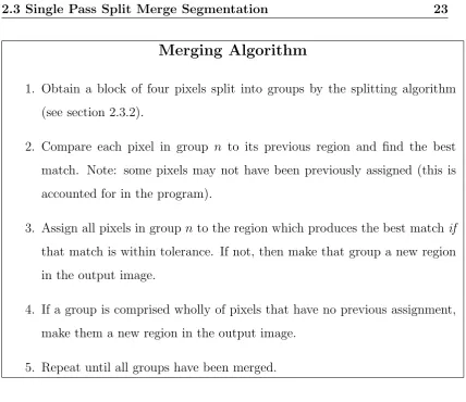
Merging Algorithm
1. Obtain a block of four pixels split into groups by the splitting algorithm (see section 2.3.2).
2. Compare each pixel in group n to its previous region and find the best match. Note: some pixels may not have been previously assigned (this is accounted for in the program).
3. Assign all pixels in groupn to the region which produces the best match if that match is within tolerance. If not, then make that group a new region in the output image.
4. If a group is comprised wholly of pixels that have no previous assignment, make them a new region in the output image.
[image:41.595.113.542.70.440.2]5. Repeat until all groups have been merged.
Figure 2.3: The merging algorithm as implemented
Figure 2.4: The orientation of the pixels in the four pixel block. This orientation
is also used in the final program
2.3.2
Splitting Algorithm
In order to successfully employ merging, it was necessary to select a small section of the image to split, as discussed above. Having done this, the split regions could be merged back into the larger image, thus creating regions.
The section to be split is a square of n = 4 pixels, the top left hand pixel being the current location in the main image 3 (see figure 2.2). This four pixel block
is now split according to the dissimilarity of the pixels. Now this seems fairly straightforward, simply see how dissimilar the pixels are and split accordingly. Unfortunately, a more rigorous definition is needed than “dissimilar”, dissimilar to what or whom? It was exceedingly difficult to find a good criterion to distinguish between varying pixels, especially as the various sources studied were annoyingly vague on the subject. Several approaches were tried, but most sources remained exasperatingly silent on just how one is supposed to assess dissimilarity.
Initially, this was not judged to be of much importance. The main reference for this topic, (Sonka et al. 1994), did not even discuss how the splitting was 3 There is nothing especially magical about four pixels, virtually any conglomeration of
2.3 Single Pass Split Merge Segmentation 25
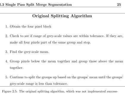
Original Splitting Algorithm
1. Obtain the four pixel block
2. Check to see if range of grey-scale values are within tolerance. If they are, make all four pixels part of the same group and stop.
3. Find the grey-scale mean.
4. Group pixels below the mean together and group those above the mean together.
[image:43.595.118.539.63.378.2]5. Continue to split the groups up based on the groups’ mean until the groups’ grey-scale range is less than tolerance.
Figure 2.5: The original splitting algorithm, which was not implemented
success-fully
to be accomplished. Clearly the working area was too small for the large scale splitting methods described in previous sections. Because of this gap, there grew the erroneous belief that any slack in the splitting would be picked up by the subsequent merging. Out of this grew the first splitting algorithm, discussed below (readers disinterested in a method that did not work and why it failed should skip to section 2.3.2).
Original Algorithm
Once obtained, the grey-scale values of the four pixel block were examined and a mean grey-scale value and grey-scale range found. If the range is less than a tolerance, all four pixels are labeled as one group and the splitting algorithm is ended. If not, then the four pixels are divided based on the mean. All those falling below the mean comprise one group, while all those above the mean comprise the other group. This process was continued in the subgroups until the grey-scale range in the subgroups was less than the tolerance.
This appears a complex and difficult process. Why not just compare each pixel to each other pixel? There are after all, only six comparisons to make. Unfortunately this option, in addition to being difficult to code successfully, creates an additional problem. Suppose that one has determined that pixel A and B are similar, A
andC may also be similar, yetCand B may be dissimilar. Which pixel to assign to a given group may end up being a matter of where the algorithm started first, thus creating different segmentation results for each order. This is clearly unsatisfactory.
Having thus split the four pixels into their component groups (a minimum of one and a maximum of four separate groups), one now had labels for each pixel in the group indicating it’s relationship with the other pixels in the four pixel set. These labels were then utilised in the merge section of the algorithm.
This was a complicated and fairly arbitrary process. However it did function after a fashion, the algorithm ran without computational error and, when combined with the merging algorithm (see section 2.3.1), produced a segmented image that appeared to correspond to the objects in view. It was only after the introduction of centroid calculations and tracking, much later (see section 4.4) that it became obvious that something was very wrong with the original method.
2.3 Single Pass Split Merge Segmentation 27
much warning. The reason why this was not picked up much earlier was that the edges of the regions were fairly stable, although they tended randomly fragment inside. Thus, while being difficult to spot through observation, a unacceptable randomness was being introduced into the segmentation process.
Long hours of painful and tedious investigation later, it became apparent that the problem was with the splitting algorithm. The original splitting algorithm, as described in figure 2.5, functioned on means. Splitting the four pixel block was accomplished by comparing the individual pixels to the mean of their prospective groups. Unfortunately, this method contained a very large logical flaw. If two pixels A and B were close together, close enough that they were obviously part of the same group, it was thought that they would be assured assignment to the same group. However if they lay on opposite sides of the mean, they would be irrevocably split into the upper and lower groups. This meant that an artifi-cial barrier could conceivably be created in the middle of the four pixel block. This barrier may, or may not be re-merged in the merging stages. It was this unfortunate possibility that was introducing a random divide into the finished regions.
Ironically, this problem was considered (although its true importance was not full recognised) early in the project. However it was overshadowed by the need to determine what to do if A and B are a group and A and C are a group, but C
and B are not (as discussed above). Essentially, it was thought that the initial method was the best compromise in dealing with a difficult situation. For some considerable time, no better answer could be formulated.
Final Algorithm
Figure 2.6: The various combinations possible with a four by four pixel block. Note
2.3 Single Pass Split Merge Segmentation 29
With four pixels, simple observation showed that there is a maximum of sixteen different patterns possible. Further investigation shows that there are actually fifteen for the purposes of this project (see figure 2.6). Thus, regardless of the pixel values they must form one of these patterns. Viewed from this perspective pixel similarity is simply a problem of finding which of the sixteen is the best match.
This may seem simple, but it is in fact an exacting and demanding process. One must be careful not to be too demanding in the criteria that decides the pattern match, or it is entirely possible that no match will be found (nothing will exactly fit the search if the criteria are defined too narrowly). Once again the problem of A, B vs A, C appears. The logic needs to be sufficiently rigorous to prohibit random edges from being formed, yet adequately flexible so a pattern is eventually made.
The best way to achieve this was found after much experimentation and revolves around comparison of differences. The crucial decider of homogeneity is the difference between each pixel. Once this is grasped, one can easily find the six difference combinations for the four pixel block. It is these differences, A−B,
A−C, A−D, C−D, B −C and B −D, that are used to form that basis of the decision making process. Once they have been computed (note that it is the absolute difference, negatives are not used), a set of comparisons are used. To prevent the logic from becoming to rigid, only the most desired patterns were explicitly defined.
become a new region, at least temporarily. Thus all combinations that left this pixel in a group of one were undesirable, this included combinations v, xi, xiii, xivand xvi. Therefore these were at the bottom of the list.
Considering the above in reverse, the most desirable combinations were those that maintained pixel D in as large a group as possible. As can be seen in figure 2.6, these sets were: i, iv, vi and vii followed by ii, iii, viii, x and xii through xv. The selection logic was arranged so that these best and the most distinctive candidates were looked for first, with explicit requirements. Following this several layers of less rigorous logic followed with the least desired combinations at the bottom, for groups that failed all other tests.
The initial tests were simple, using the six differences and the image tolerance (see section 2.3.1). If the largest difference was less than the tolerance, then all pixels were of a group, if the smallest difference was greater, they were all separate. Following this ii, iii, xiii and ix were also searched for explicitly, using exacting
if statements that ensured the derided shapes existed. Then an if statement was constructed for each difference. If the considered difference was less than tolerance, then the number of shapes the block could be was restricted. For example if A−B < T then all combinations that splitA and B can be ignored. This list of probables can be reduced still further if once considers the combination that were rejected to reach this point. Often, there was only one possibility. In cases where there were more, they were selected by nested if, else statements that used other differences and guaranteed preference to preferred shapes. Thus an appropriate assignment was ensured, and all four pixel blocks assigned some split pattern.
2.4 Image Pre-Processing 31
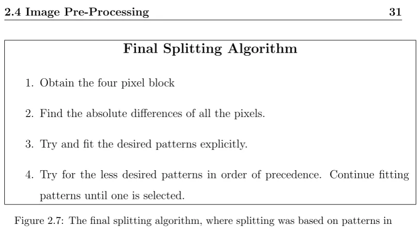
Final Splitting Algorithm
1. Obtain the four pixel block
2. Find the absolute differences of all the pixels.
3. Try and fit the desired patterns explicitly.
[image:49.595.110.541.66.309.2]4. Try for the less desired patterns in order of precedence. Continue fitting patterns until one is selected.
Figure 2.7: The final splitting algorithm, where splitting was based on patterns in
order of precedence
2.4
Image Pre-Processing
The output of the segmentation process described above was sufficient all one wished was to subdivide a still image. However, upon implementation it became aspirant that the process was rather too simple. Regions representing immobile objects tended to grow and shrink in an apparently random fashion. This was attributed to insufficient flexibility in the program relative to variable conditions in the image.
2.4.1
Noise Removal and Image Smoothing
The creation of regions was found to be highly susceptible to the image noise. As the initial camera was not of the highest quality (it was the stock machine attached to the author’s laptop), steps had to be taken to alleviate the noise.
Some simple investigations4 showed that the OpenCV library contained some 4It in necessary to confess that the research in this area was not as in depth as others. This
preexisting functions for image smoothing.
Image smoothing involves subjecting the image to a controlled blur, this smooths out the random high points in the image caused my noise (Bradski & Kaehler 2008). The difficulty with this, as might be imagined, is that important features can become obscured if the blur is severe enough. Initially, a standard Gaussian blur was used however it was found that the more complicated Bilateral filter would be able to perform a Gaussian blur on the interior of objects whilst pre-serving the edges, the effect of which is “typically to turn an image into what appears to be a watercolor painting of the same scene. This can be useful as an aid to segmenting the image” (Bradski & Kaehler 2008). This quote was taken at face value and a moderate Bilateral filter installed before the segmentation algorithm and run once over each frame.
2.4.2
Finding a Tolerance
All the segmentation methods described above required some form of homogeneity criterion or tolerance to work. This is yet another area upon which the literature was annoyingly glib. Because of this, several methods were tried to find a truly flexible and accurate tolerance. Indeed, for some time it was believed that one of the key problems with the regions stability was lack of a good tolerance value.
In original versions, the tolerance value was fixed to an arbitrary number at the start of the program. Clearly this was an unacceptable situation. Changing light patterns, movement, the intrusion of darker or lighter objects into the screen all had the effect of changing the relationship between various objects.
2.4 Image Pre-Processing 33
While it is easy to comprehend the necessity for such a scheme, the literature provides very few explicit references regarding methodology. Most sources simply state the need for such a system, without describing the minutiae of execution. Initially, it was decided to find the maximum and minimum grey values in the given frame and set the tolerance ton% of the difference. This valuenwas found, after patient experimentation to be best set to 10%.
The disadvantage of this system is that it still contained an arbitrary quantity, the constant n. While the method was, in theory flexible, it wasn’t much of an improvement over its predecessor, as a rule it was found that all “real” images contained a 0 and 255 pixel. So in effect the value of tolerance remained static.
The final modification was to base the tolerance on the standard deviation of the image. The standard deviation is the square root of sum of the average of the squares of the distance from the mean (Moore 1995). What that cumbersome descriptor means is that standard deviation is a measure of the spread of the image pixel values. In other words, how widely separate the numerical values of the pixels are. Thus an almost black image will have a very low standard deviation while a image of many sharp, vibrantly coloured objects will have a very high one.
2.5
Potential Problems
Despite all the investigations and considerations mentioned, there remain a num-ber of potential difficulties with the implemented method. The first of these arises when the merging process is considered. In order to accurately judge which groups to merge with what regions, a tally of the total number of pixels and the total grey-scale value of each region. This enables a mean to be computed and compared to the group mean to assess merging potential.
The difficulty that arises in how this information is stored. The program creates two vectors 256 entries long. The number of each entry is the output grey-scale value of the pixels filling it. This means that if pixel A is merged to a region of output value 45, then the 45th element in vector RegionCountis incremented by one and the 45th element in vector RegionSum is increased by the original value of A. In this way an average of all pixels of value n in the output image can be kept. However, this process does not take into account region congruity. By definition (Jain et al. 1995) pixels in a region must be both homogeneous and share a common edge. This approach tallies all the pixels in all the regions that are value n in the output, as though they were in one region.
Chapter 3
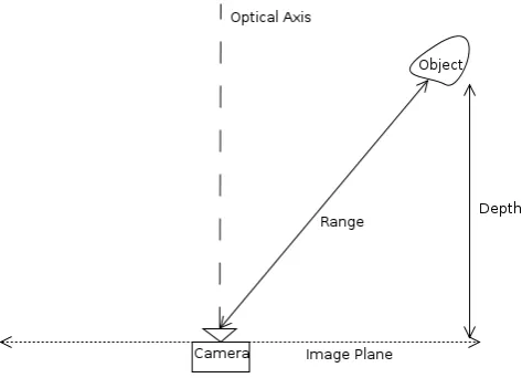
3.1 Methods of Distance Estimation 37
Figure 3.1: illustration of the difference between range and depth.
Once the image has been segmented, one might reasonably ask how can we find the location of these segmented objects, relative to the camera? Recall that the purpose of segmentation was to determine which pixels in the image belong to which object in reality. Thus there is a correspondence between the objects in the projected image and the objects before the viewer.
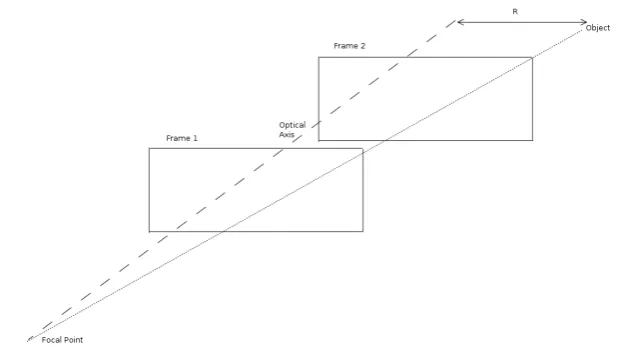
Figure 3.2: Stereo vision, using one camera and the frame difference to find depth.
3.1
Methods of Distance Estimation
The literature describes two broad methods of estimating the position and motion of an object relative to the camera. These two groups are, those based on stereo vision and those based on the evolution of the image over time (Jain et al. 1995), (Davies 1997). Obviously, true stereo vision is not an option (the focus is on monocular vision). This restriction led to the conclusion that the location of objects would have to be calculated based on analysis and information from a number of successive frames.
3.1 Methods of Distance Estimation 39
As mentioned, there are two broad categories of distance estimation. Stereo appears the most frequently and although true stereo vision was not considered, it is possible to approximate it from the difference between two frames of a moving image. Classic stereo vision involves two cameras set some distance apart. Both record the same scene but from a different perspective. The discrepancy between the two provides the basis for calculations that describe depth and range (Jain et al. 1995). Such an arrangement would be familiar to most readers in the form of human eyes and binocular optical range finders.
While this arrangement is perhaps the most intuitive of distance judging tech-niques, the focus on monocular methods render it inappropriate in this case. Nevertheless it is possible to achieve the same effect from one camera and the image sequence. This is because, for a moving scene, each frame is slightly differ-ent than the last. Thus one may approximate the stereo arrangemdiffer-ent by noting that as the scene moves, the camera is seeing the scene from a slightly different perspective (Davies 1997). This shift in perspective can be combined with some simple geometry and used to generate the distance from the camera to the point. Therefore there is now sufficient information to compute the range of any given point, if it has been tracked from frame to frame (see figure 3.2).
While potentially useful, this method suffers from one serious flaw. It cannot assess motion if that motion is directly long the optical axis (the line orthogonal to the image plane and passing through the focal point, the center of the image in effect). Examination of the equations used to compute range revealed that they fail when distance from the optical axis approaches zero (Davies 1997). This is because there ceases to be any discrepancy between the frames, the point of view becomes constant. Hence an object can approach at any speed, but if the line of approach is the optical axis, there will be no movement in the projected image plane. This means that objects approaching from directly ahead remain invisible. This clearly renders it an unsuitable method for this application.
robot was turning. At early stages, it was assumed that the hypothetical robot would be able to execute a zero point turn (also it was assumed that it would be desirable to do this). As other methods considered (especially Looming, the selected method, see section 3.2) require some forward component of motion, stereo from motion was considered an ideal alternative. As the camera turned, all objects in frame would undergo motion from one frame to the next. There would be no blind spot as described above, because all image motion vectors would have been orthogonal to the optical axis.
This effect would enable the range to be calculated while turning, providing a good estimation of range for when the rotation had ceased and other methods could be resumed. Otherwise, it was thought that the machine would have to shuffle backwards and forwards to artificially create motion and so orient itself after each rotation.
In the event, it was found that the hardware envisaged would not necessarily need to perform this maneuver. Every turn could be accompanied by some for-ward motion component. Also, it was observed (Low 15/12/2010 to October 27/10/2011) that the movement from frame to frame as the machine turned may be insufficient to enable accurate computations to be made. Thus, for these rea-sons, Looming was recommended as a preferred alternative (Low 15/12/2010 to October 27/10/2011). Nevertheless, stereo from motion remains a potentially powerful tool, especially for rotational motion.
3.2 Looming 41
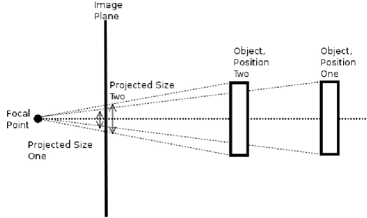
Figure 3.3: Graphical depiction of Looming using projected area.
3.2
Looming
A review of literature and certain advice, indicated that Looming is potentially the most useful method of range estimation. It possessed the potential for the most intuitive, simple results, it matched perfectly with the segmentation ap-proach and was computationally simple. Furthermore it could be easily imple-mented with monocular vision, rendering it particularly suitable for the aims of the project.
to imply the range of an object without further calculation (Raviv 1995). The quantity L is defined by the following equation,
L= dR
dt
R (3.1)
Where:
L is the Looming Value ( [time]−1)
R is the Range (m)
Thus it is evident that there is a relationship between the Looming value L, and the rangeR. Notice thatL is proportional not only to the range, but also to the rate of change of range, the approach of the object. Thus if L can be calculated another way, one could use the value ofL for any given point to imply the range of that point. Therefore, one defines L as:
L= dg dt
g (3.2)
Where g is some property of the image that may be calculated (Raviv 1995).
Recalling that Looming is based on the idea that aspects of an image region change as the real object approaches, it is possible to define L in terms of one of these changing aspects. The most obvious solution is to simply use the change in region area. Although this is possible, other aspects may be more useful. The other region properties include: irradiance, texture and blur (Raviv 1995). These four features occur repeatedly in the literature.
3.2.1
Area
3.2 Looming 43
Notice that the projected size of the object is increasing as the object approaches. Mathematically, the value Lcan be expressed as:
L= dA
dt
A (3.3)
While it is the simplest to explain and illustrate, the area method is flawed in several important ways. Firstly, the area of the regions as derived by the segmentation algorithm (see section 2.3) was found to fluctuate in practice. When the segmentation program was run, the area of the segments was not stable enough to produce consistent values ofA(this is discussed further in section 5.2). Secondly, and more importantly, the area method is limited by the field of view (Sahin & Gaudiano 1998).
In order to accurately compute L from area or apparent size, one must have the region in question fully in the frame in at least one dimension. If an object approaches so that it begins to move out of the field of view, the total number of pixels in that region begins to decline. Even though the object is still Looming larger and approaching, the number of pixels that are used to represent it is decreasing as the region slides off the edge of the image. Thus the Looming value
L would be decreasing even as the object is actually Looming larger.
This can be overcome to some degree by using length instead of area to measureL
3.2.2
Irradiance
The illumination approach to Looming is yet another method of estimating the range through the use of image data. In this case the image data used is the temporal change in image irradiance (Raviv & Joarder 2000). Where “irradiance” is some measure of the reflected light off the object surface. The idea is that this will noticeably alter as the camera approaches the object, thus providing the Looming indicator. The literature indicates that there are three approaches to this method. All however, rely on the assumption that the surfaces in view are Lambertian surfaces.
A Lambertian surface is essentially a surface that appears equally bright from all viewing directions (Jain et al. 1995). This was considered a risky assumption, considering that many surfaces in the field of view may not be strictly Lambertian. This was a key reason in the decision to abandon this line of research.
The differing methods are based around the movement of the light source. In the first case, the light source is stationary, while the camera moves. This is perhaps the most apt approach to the problem for a mobile robot (assuming the machine is not carrying its own light source). However, the method described in (Raviv & Joarder 2000) makes no mention of the appearance of new light sources, as would certainly happen as the machine moves down a corridor. Perhaps more importantly this method requires the calculation of the angleθ. This is the angle between the surface normal and the optical axis. While possible, the computation of this angle was felt initially to be too complex a task in comparison with other methods.
3.2 Looming 45
These complexities ensured that Looming through irradiance was abandoned early as a potential method. Although they could probably be solved, other methods were considered easier to implement and more reliable in operation.
3.2.3
Texture
Looming through texture is yet another method of gauging object approach. Fundamentally similar to all other Looming methods, the texture approach takes as its changing variable the texture density. The idea is that as one approaches, the texture of an object becomes more intricate.
To gauge this, one defines a “textel” (sometimes given other, similar names) as a description of the texture pattern. The assumption is that any texture is comprised of repeating units. These “textels” in summation comprise the entire pattern (Pietik¨ainen 2000). As described in (Raviv 1995), the increase in “textels” indicates an increase in the intricacy of the pattern and thus the approach of the object. The general idea being that the more complexity one can see in an object, the closer it must be.
3.2.4
Blur
The final Looming method mentioned in the literature is Looming through radius of blur. If one considers a camera focused at a point, all points at a different distance from the camera than the focused point will exhibit some degree of de-focus or blur. The edges of each object will be fuzzy in a way which is proportional to its distance from the camera. However, if the camera is focused at infinity, all points not at infinity will exhibit some degree of blur, proportional to their proximity to the camera. This means that objects in the far distance will appear almost clear, while objects in the foreground will be badly out of focus. The evolution of this optical blur magnitude over time can be used to compute the Looming value (Raviv 1995).
L= dr dt
r (3.4)
Equation 3.4 illustrates the relationship between the Looming value L and the radius of blur r (Raviv 1995). However, to employ this equation, it becomes necessary to somehow rigorously define blur. Some value which describes blur at a given point must be obtained from the image data.
It transpires that the value in question can be taken as the radius of the point spread function (PSF). This is the function which describes the blur circle and when convolved with the original image produces the blur (Subbarao 1987). One can say thatr is some quantity that can be obtained from this function (Raviv & Joarder 2000). If this value ofrcan be recovered, it could be possible to compute
L.
3.2 Looming 47
Figure 3.4: The Gaussian curve, showing standard deviation (σ) and the true radius of blur
standard deviation (De Veaux, Velleman & E. 2004) as r. Note that it is not
r, but rather proportional to r, however it is always proportional by the same relationship and is thus an acceptable measure of r (Raviv 1995).
This relationship is demonstrated in figure 3.4. Notice that the true radius of blur is where the curve becomes practically insignificant.
g(n, σ) = √1
2πσexp
− n
2
2σ2
(3.5)
Where,
n is the pixel range around the current position.
σ is the standard deviation of the Gaussian distribution.
Notice in equation 3.5 there is only one variable σ. In this application it is as-sumed that the blur is symmetric. That is, it can be modeled by a rotated one dimensional Gaussian. This means that only one value, σ need be recovered. There exist models for two dimensional Gaussian blur, with two orthogonal val-ues σ1 and σ2 (Luxen & F¨orstner 2002), however this was felt to add needless
suffi-Figure 3.5: Plot of various step functions representing the region edge with varying
degrees of ideal blur. f(x) is the original step, withb(x) being the camera’s blurred edge and ba(x) andbb(x) being the re-blurred edges.
cient. Naturally, this assumes that the blur is symmetric. At this stage it will be considered to be so, this will have to be tested in implementation.
At this point the question became how to recover this value from the image data. Research has indicated that this can be done several ways. Firstly, there exist iterative methods (Hu & de Haan 2006). These were excluded from the investigation on the grounds of computational complexity. It is important to recall that reducing computational complexity is critical, given the real time project specification.
Further reading indicated the existence of other low cost blur estimation algo-rithms, especially one based on blurring the image several times with a known blur (see (Hu & de Haan 2006)).
[image:66.595.158.397.107.295.2]3.2 Looming 49
Figure 3.6: Plot of Rmax values recovered in Note the symmetrical nature of the
plot around the region boundary.
Consider the step function description of an ideal edge. Ideally, between one object and another, there is a sharp demarcation. This demarcation could be used in an edge detection algorithm to describe the object edge (see section 2.2.2). Ideally this is a step, as shown by the f(x) line in figure 3.5, however in a real image, the edges of objects are seldom so crisp. There will be a certain amount of blur present. If the camera is de-focused, as discussed above, this blur will be guaranteed. This causes a “softening” of the edge step function, as illustrated by theb(x) curve in figure 3.5. Notice that there is no longer a sharp drop between regions, but that the edge has been rounded. pixels of a medium value now lie between the two regions. This effect becomes more pronounced as the blur becomes more severe (lines ba(x) and bb(x) in figure 3.5)
It is important to note that the values illustrated in 3.5 represent the ideal blur edges. This is what would be produced if an ideal Gaussian blur was used. Math-ematically these curves exhibit the perfect result. However, when implemented they were not so exact (see figure 5.11).
can be produced by performing a convolution on the original f(x) step with a Gaussian function. The Gaussian (equation 3.5), can be expressed as:
g(n, σ) = √1
2πσexp
− n
2
2σ2
(3.6)
Where n is the position in the image and σ is the standard deviation. From this it is possible to show that 1 the blared step edge will be:
b(x) = X n∈I
f(x−n)g(n, σ)
= A
2 1 +
x
X
n=−x
g(n, σ) !
+B, x≥0
A
2 1−
x
X
n=−x
g(n, σ) !
+B, x≤0
(3.7)
WhereAandB are the constants that define the idealised step function shown in figure 3.5. The original Gaussian blur is now convolved with two new blurs. Using the property illustrated in equation 3.2.4, the new blurred edgebax is illustrated in equation 3.2.4.
g(n, σ1)∗g(n, σ2) = g(n,
q
σ2
1−σ22) (3.8)
ba(x) =
A
2 1 +
x
X
n=−x
g(n,pσ2−σ2
a)
!
+B, x≥0
A
2 1−
x
X
n=−x
g(n,pσ2−σ2
a)
!
+B, x≤0
(3.9)
3.2 Looming 51
The same equation can be used to describe the result of the second re-blur, except
σb is used instead ofσa. Note that the two convolutions are separate operations, the initial blurred image is not convolved sequentially. Thus there are two re-blurred images that both started as the initial image.
The next step is to make the final operation independent of the constantsA and
B. To do this, the ratio of