This is a repository copy of A system’s wave function is uniquely determined by its
underlying physical state.
White Rose Research Online URL for this paper:
http://eprints.whiterose.ac.uk/110595/
Version: Accepted Version
Article:
Colbeck, Roger Andrew orcid.org/0000-0003-3591-0576 and Renner, Renato (2017) A
system’s wave function is uniquely determined by its underlying physical state. New
Journal of Physics. 013016. pp. 1-12. ISSN 1367-2630
https://doi.org/10.1088/1367-2630/aa515c
[email protected] https://eprints.whiterose.ac.uk/
Reuse
This article is distributed under the terms of the Creative Commons Attribution (CC BY) licence. This licence allows you to distribute, remix, tweak, and build upon the work, even commercially, as long as you credit the authors for the original work. More information and the full terms of the licence here:
https://creativecommons.org/licenses/
Takedown
If you consider content in White Rose Research Online to be in breach of UK law, please notify us by
Roger Colbeck1,∗ and Renato Renner2,†
1
Department of Mathematics, University of York, YO10 5DD, UK
2
Institute for Theoretical Physics, ETH Zurich, 8093 Zurich, Switzerland (Dated: January 13, 2017)
We address the question of whether the quantum-mechanical wave function Ψ of a system is uniquely determined by any complete description Λ of the system’s physical state. We show that this is the case if the latter satisfies a notion of “free choice”. This notion requires that certain experimental parameters—those that according to quantum theory can be chosen independently of other variables—retain this property in the presence of Λ. An implication of this result is that, among all possible descriptions Λ of a system’s state compatible with free choice, the wave function Ψ is as objective as Λ.
I. INTRODUCTION
The quantum-mechanical wave function, Ψ, has a clear operational meaning, specified by the Born rule [1]. It asserts that the outcome X of a measurement, defined by a family of projectors {Πx}, follows a distribution
PX given by PX(x) = hΨ|Πx|Ψi, and hence links the wave function Ψ to observations. However, the link is probabilistic: even if Ψ is known to arbitrary precision, we cannot in general predictX with certainty.
In classical physics, such indeterministic predictions are always a sign of incomplete knowledge.1 This raises the question of whether the wave function Ψ associated to a system corresponds to anobjective property of the sys-tem, or whether it should instead be interpreted subjec-tively, i.e., as a representation of our (incomplete) knowl-edge about certain underlying objective attributes. An-other alternative is to deny the existence of the latter, i.e., to give up the idea of an underlying reality completely.
Despite its long history, no consensus about the in-terpretation of the wave function has been reached. A subjective interpretation was, for instance, supported by the famous argument of Einstein, Podolsky and Rosen [2] (see also [3]) and, more recently, by information-theoretic considerations [4–6]. The opposite (objective) point of view was taken, for instance, by Schr¨odinger (at least initially), von Neumann, Dirac, and Popper [7–9].
To turn this debate into a more technical question, one may consider the following gedankenexperiment: As-sume you are provided with a set of variables Λ that are intended to describe the physical state of a system. Sup-pose, furthermore, that the set Λ iscomplete, i.e., there is nothing that can be added to Λ to increase the accuracy of any predictions about the outcomes of measurements
∗[email protected] †[email protected]
1
For example, when we assign a probability distributionP to the outcomes of a die roll,P is not an objective property but rather a representation of our incomplete knowledge. Indeed, if we had complete knowledge, including for instance the precise movement of the thrower’s hand, the outcome would be deterministic.
Ψ-epsistemic Ψ-ontic
λ
ψ2
ψ1 ψ3
ψ2
ψ1 ψ3
ψ2
ψ1 ψ3
λ
ψ2
ψ1 ψ3
Ψ is complete Ψ is not complete
λ
λ
PΛ|ψi(λ) PΛ|ψi(λ)
[image:2.595.319.567.222.386.2]PΛ|ψi(λ) PΛ|ψi(λ)
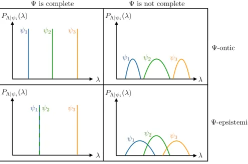
FIG. 1: The different possible roles of the wave function Ψ. A model that uses a variable Λ to describe a system’s physi-cal state can be either Ψ-ontic or Ψ-epistemic, depending on whether or not the wave function Ψ is uniquely determined by Λ (which takes values denoted byλ). Conversely, the rel-evant parts of Λ may be determined by Ψ, in which case Ψ is complete. Using free choice (with respect to an appropriate causal order), [17] rules out the right column, [16] rules out the bottom left case, and the present paper (as well as [14], based on different assumptions) rules out the bottom row.
on the system. If you were now asked to specify the wave function Ψ of the system, would your answer be unique? If so then Ψ is a function of the variables Λ and hence as objective as Λ. The model defined by Λ would then be called Ψ-ontic [10]. Conversely, the existence of a complete set of variables Λ that does not determine the wave function Ψ would mean that Ψ cannot be inter-preted as an objective property. Λ would then be called Ψ-epistemic (see Fig. 1).2
2
2
In a seminal paper [14], Pusey, Barrett and Rudolph showed that any complete model Λ is Ψ-ontic if it satisfies an assumption, termed “preparation independence”. It demands that Λ consists of separate variables for each subsystem, e.g., Λ = (ΛA,ΛB) for two subsystems SA
andSB, and that these are statistically independent, i.e.,
PΛAΛB =PΛAPΛB, whenever the joint wave function Ψ of the total system has product form, i.e., Ψ = ΨA⊗ΨB.
Here we show that the same conclusion can be reached without imposing any internal structure on Λ. In more detail, our argument relies on the concept of free choice, which can only be defined with reference to an ordering, called here acausal order3. More precisely, we prove that Ψ is a function of any complete set of variables that are compatible with free choice with respect to the causal or-der of Figure 3 (see later for more details). This is stated as Corollary 1. The free choice assumption used cap-tures the idea that experimental parameters, e.g., which state to prepare or which measurement to carry out, can be chosen independently of all other information (rele-vant to the experiment), except for information that is created after the choice is made, e.g., measurement out-comes. While this notion is implicit in quantum theory, we demand that it also holds in the presence of Λ.4
The proof of our result is inspired by our earlier work [16] in which we observed that the wave function Ψ is uniquely determined by any complete set of vari-ables Λ, provided that Ψ is itself complete (in the sense described above). Together with the result of [17], in which we showed that Ψ is complete, we can conclude that the wave function Ψ is uniquely determined by Λ.
The difference in the present work is that we can cir-cumvent one of the aspects of quantum theory required by the argument in [17]. In particular, here we prove that Ψ is determined by Λ without requiring that any quan-tum measurement on a system corresponds to a unitary evolution of an extended system. Being based on weaker assumptions, the resulting no-go theorem is stronger. Furthermore, the argument that the wave function Ψ is complete is quite involved and a beneficial feature of the present work is that we circumvent it5.
II. THE UNIQUENESS THEOREM
Our argument refers to an experimental setup where a particle emitted by a source decays into two, each of which is directed towards one of two measurement de-vices (see Fig. 2). The measurements that are performed
doubt on this possibility (see, for example, [11–13]).
3
This should not be confused with acausal structure as used in e.g. [15].
4
Free choice of certain variables is also implied by the preparation independence assumption used in [14], as discussed below.
5
Note, however, that the assumptions used in this work do not allow us to conclude that Ψ is complete.
decay
source
measurement measurement
{Πax} {Πby}
X Y
A B
U
Λ
[image:3.595.352.522.49.314.2]Ψ
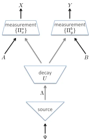
FIG. 2:The experimental setup. The proof of the uniqueness theorem relies on a thought experiment where a source takes as input a description of a wave function Ψ and prepares a particle in a corresponding state (which, in a general model, is described by a variable Λ). The particle then decays into two parts, which are measured at separate locations. A and
B determine the measurements that are applied to the two parts, andX andY are the respective outcomes.
depend on parametersAandB, and their respective out-comes are denotedX andY.
Quantum theory allows us to make predictions about these outcomes based on a description of the initial state of the system, the evolution it undergoes and the mea-surement settings. For our purposes, we assume that the quantum state of each particle emitted by the source is pure, and hence specified by a wave function6. As we will consider different choices for this wave function, we model it as a random variable Ψ that takes as values unit vectors ψ in a complex Hilbert space H. Furthermore, we take the decay to act like an isometry, denoted U, from H to a product space HA⊗ HB. Finally, for any
choices a and b of the parameters A and B, the mea-surements are given by families of projectors {Πa
x}x∈X and {Πb
y}y∈Y on HA and HB, respectively. The Born
rule, applied to this setting, now asserts that the joint probability distribution ofX andY, conditioned on the
6
B A
X
Ψ Y
[image:4.595.138.218.50.178.2]Λ
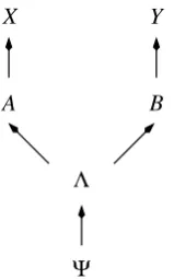
FIG. 3: The causal order. Free choice is only well defined if one specifies a causal order, i.e., a preorder relation on the set of variables relevant to the experiment. The causal order we use is motivated by the arrangement of variables in the experiment depicted by Fig. 2 in relativistic space time.
relevant parameters, is given by
PXY|ABΨ(x, y|a, b, ψ) =hψ|U†(Πax⊗Πby)U|ψi. (1)
To model the system’s “physical state”, we introduce an additional random variable Λ. We do not impose any structure on Λ (in particular, Λ could be a list of values). We will consider predictionsPXY|ABΛ(x, y|a, b, λ)
condi-tioned on any particular valueλof Λ, analogously to the
predictions based on Ψ according to the Born rule (1).
To define the notions offree choice andcompleteness,
as introduced informally in the introduction, we take as motivation that any experiment takes place in spacetime
and therefore has acausal order7. For example, the
mea-surement settingAis chosen before the measurement
out-comeX is obtained. This may be modelled
mathemati-cally by a preorder relation8, denoted , on the relevant
set of random variables. While our technical claim does not depend on how the causal order is interpreted phys-ically, it is intuitive to imagine it being compatible with
relativistic spacetime. In this case,A X would mean
that the spacetime point whereX is accessible lies in the
future light cone of the spacetime point where the choice
Ais made.
For our argument we consider the causal order defined by the transitive completion of the relations
Ψ Λ, Λ A, Λ B, A X, B Y (2)
(cf. Fig. 3). This reflects, for instance, that Ψ is chosen at
the very beginning of the experiment, and thatAandB
are chosen later, right before the two measurements are
carried out. Note, furthermore, thatA6 Y andB6 X.
With the aforementioned interpretation of the relation
7
In previous work we sometimes called this achronological struc-ture[18].
8
Apreorder relationis a binary relation that is reflexive and tran-sitive.
in relativistic spacetime, this would mean that the two measurements are carried out at spacelike separation.
Using the notion of a causal order, we can now specify
mathematically what we mean by free choices and by
completeness. We note that the two definitions below should be understood as necessary (but not necessarily sufficient) conditions characterising these concepts. Since they appear in the assumptions of our main theorem, our result also applies to any more restrictive definitions. We remark furthermore that the definitions are generic, i.e., they can be applied to any set of variables equipped with a preorder relation.9
Definition 1. When we say that a variableA is a free choice from a set A (w.r.t. a causal order) this means that the support ofPAcontainsAand thatPA|A6 ↑=PA whereA6↑ is the set of all random variablesZ (within the
causal order) such thatA6 Z.
In other words, a choice A is free if it is uncorrelated
with any other variables, except those that lie in the
fu-ture of A in the causal order. For a further discussion
and motivation of this notion we refer to Bell’s work [19] as well as to [20].
Crucially, we note that Definition 1 is compatible with the usual understanding of free choices within quantum theory. For example, if we consider our experimental setup (cf. Fig. 2) in ordinary quantum theory (i.e., where there is no Λ), the initial state Ψ as well as the
measure-ment settingsA and B can be taken to be free choices
w.r.t. Ψ A, Ψ B, A X, B Y (which is the
causal order defined by Eq. 2 with Λ removed).
Definition 2. When we say that a variable Λ iscomplete (w.r.t. a causal order)this means that10
PΛ↑|Λ=PΛ↑|ΛΛ↓
where Λ↑ and Λ↓ denote the sets of random variables Z
(within the causal order) such that Λ Z and Z Λ,
respectively.
Completeness of Λ thus implies that predictions based
on Λ about future values Λ↑cannot be improved by
tak-ing into account additional information Λ↓ available in
the past.11 Recall that this is meant as a necessary
cri-terion for completeness and that our conclusions hold for any more restrictive definition. For example, one may replace the set Λ↑ by the set of all values that are not in the past of Λ.
9
They are therefore different from notions used commonly in the context of Bell-type experiments, such as parameter indepen-denceandoutcome independence. These refer explicitly to mea-surement choices and outcomes, whereas no such distinction is necessary for the definitions used here.
10
In other words, Λ↓→Λ→Λ↑is a Markov chain.
11
4
We are now ready to formulate our main result as a theorem. Note that, the assumptions of the theorem as well as its claim correspond to properties of the joint probability distribution ofX, Y,A,B, Ψ and Λ.
Theorem 1. Let Λ andΨbe random variables and as-sume that the support ofΨcontains two wave functions,
ψ and ψ′, with |hψ|ψ′i|<1. If for any isometryU and
measurements{Πa
x}xand{Πby}y, parameterised bya∈ A andb∈ B, there exist random variablesA,B,X and Y
such that
1. PXY|ABΨ satisfies the Born rule (1);
2. A andB are free choices fromAandB, w.r.t.(2);
3. Λ is complete w.r.t. (2)
then there exists a subset L of the range of Λ such that
PΛ|Ψ(L|ψ) = 1andPΛ|Ψ(L|ψ′) = 0.
The theorem asserts that, assuming validity of the Born rule and freedom of choice, the values taken by any complete variable Λ are different for different choices of the wave function Ψ. This implies that Ψ is indeed a function of Λ.
To formulate this implication as a technical statement,
we consider an arbitrary countable12 setS of wave
func-tions such that |hψ|ψ′i| < 1 for any distinct elements
ψ, ψ′ ∈ S.
Corollary 1. Let Λ andΨbe random variables with Ψ
taking values from the set S of wave functions. If the conditions of Theorem 1 are satisfied then there exists a function f such that Ψ =f(Λ)holds almost surely.
The proof of this corollary is given in Appendix A.
III. PROOF OF THE UNIQUENESS THEOREM
The argument relies on specific wave functions, which
depend on parameters d, k ∈ N and ξ ∈ [0,1], with
k < d. They are defined as unit vectors on a
prod-uct space HA⊗ HB, where HA and HB are (d+
1)-dimensional Hilbert spaces equipped with an orthonor-mal basis{|ji}d
j=0,13
φ= √1
d
d−1
X
j=0
|ji|ji (3)
φ′= √1
k
ξ|0i|0i+
k−1
X
j=1
|ji|ji+p1−ξ2|di|di. (4)
12
The restriction to a countable set is due to our proof technique. We leave it as an open problem to determine whether this re-striction is necessary.
13
We use here the abbreviation|ji|jifor|ji ⊗ |ji.
Lemma 1. For any 0≤α <1 there existk, d∈Nwith
k < dandξ∈[0,1]such that the vectorsφandφ′defined
by (3) and (4) have overlaphφ|φ′i=α.
Proof. Ifα= 0, setk= 1,d= 2 andξ= 0. Otherwise, setd≥1/(1−α2),k=⌈α2d⌉andξ=α√kd−k+ 1, so
that ξ∈ [0,1] and hφ|φ′i =α. Furthermore, the choice
ofdensures thatα2d+ 1≤d, which impliesk < d.
Furthermore, for any n ∈ N, we consider projective
measurements{Πa
x}x∈Xd and{Πby}y∈Xd onHA andHB,
parameterised bya∈ An ≡ {0,2,4, . . . ,2n−2} andb∈
Bn ≡ {1,3,5, . . . ,2n−1}, and with outcomes in Xd ≡
{0, . . . , d}. For x, y ∈ {0, . . . , d−1}, the projectors are
defined in terms of the generalised Pauli operator, ˆXd ≡
Pd−1
l=0 |lihl⊕1|(where⊕denotes addition modulod) by
Πax≡( ˆXd)
a
2n|xihx|( ˆX†
d)
a
2n (5)
Πby ≡( ˆXd)
b
2n|yihy|( ˆX†
d)
b
2n . (6)
We also set Πa
d= Πbd=|dihd|.
The outcomes X and Y will generally be correlated.
To quantify these correlations, we define14
In,d(PXY|AB)≡2n− d−1
X
x=0
PXY|AB(x, x⊕1|0,2n−1)
−X
a,b
|a−b|=1 d−1
X
x=0
PXY|AB(x, x|a, b).
For the correlations predicted by the Born rule for
the measurements {Πa
x}x∈Xd and {Πby}y∈Xd applied to
the state φ defined by (3), i.e., PXY|AB(x, y|a, b) =
hφ|Πa
x⊗Πby|φi, we find (see Appendix B)
In,d(PXY|AB)≤
π2
6n . (7)
The next lemma shows thatIn,dgives an upper bound
on the distance of the distributionPX|AΛfrom a uniform
distribution over {0, . . . , d−1}. The bound holds for any random variable Λ, provided the joint distribution PXYΛ|AB satisfies certain conditions.
Lemma 2. Let PXY ABΛ be a distribution that
satis-fies PXΛ|AB = PXΛ|A, PYΛ|AB = PYΛ|B and PABΛ =
PAPBPΛ with supp(PA) ⊇ An and supp(PB) ⊇ Bn.
Then
Z
dPΛ(λ) d−1
X
x=0
PX|AΛ(x|0, λ)−
1 d
≤
d
2In,d(PXY|AB).
14
Note that the first sum corresponds to the probability that
(Although our proof deals with the general case, the main ideas can be seen by working through the analogous argument in the slightly simpler (but less general) case in which Λ is discrete, so that “R
dPΛ(λ)” is replaced by
“P
λPΛ(λ)”.)
The proof of Lemma 2 is given in Appendix C. It generalises an argument described in [17], which is in turn based on work related to chained Bell inequalities [21, 22] (see also [23, 24]).
We have now everything ready to prove the uniqueness theorem.
Proof of Theorem 1. Let α, γ ∈ R such that eiγα = hψ|ψ′i. Furthermore, letk, d, ξbe as defined by Lemma 1,
so that hφ|φ′i = α. Then there exists an isometry U
such that U ψ = φ and U ψ′ = eiγφ′ (see Lemma 3
of Appendix D).15 Now let n ∈ N and let A, B, X
and Y be random variables that satisfy the three
con-ditions of the theorem for the isometry U and for the
projective measurements defined by (5) and (6), which
are parameterised by a ∈ An and b ∈ Bn, respectively.
According to the Born rule (Condition 1), the distribu-tionPXY|ABψ ≡PXY|ABΨ(·,·|·,·, ψ) conditioned on the
choice of initial state Ψ =ψcorresponds to the one
con-sidered in (7), i.e.,
In,d(PXY|ABψ)≤
π2
6n . (8)
Note that PA|BΨPYΛ|ABΨ = PAYΛ|BΨ =
PA|BYΛΨPYΛ|BΨ. Freedom of choice (Condition 2)
implies that PA|BΨ = PA|BYΛΨ. It follows that
PYΛ|ABΨ = PYΛ|BΨ. By a similar reasoning, we also
have PXΛ|ABΨ = PXΛ|AΨ. The freedom of choice
condition also ensures that PABΛ|Ψ = PAPBPΛ|Ψ with
supp(PA)⊇ Anand supp(PB)⊇ Bn. We can thus apply
Lemma 2 to give, with (8),
Z
dPΛ|ψ(λ) d−1
X
x=0
PX|AΛΨ(x|0, λ, ψ)−
1 d
≤
dπ2
12n .
Considering only the termx=k (recall thatk < d) and
noting that the left hand side does not depend onn, we
have
Z
dPΛ|ψ(λ)
PX|AΛΨ(k|0, λ, ψ)−
1 d = 0
(otherwise, by taking n sufficiently large, we will get a
contradiction with the above). LetLbe the set of all
el-ementsλfrom the range of Λ for whichPX|AΛΨ(k|0, λ, ψ)
is defined and equal to 1
d. The above implies that
PΛ|Ψ(L|ψ) = 1. Furthermore, completeness of Λ
15
IfHhas a larger dimension thanHA⊗HB(e.g., becauseHis in-finite dimensional) then we can consider an (inin-finite dimensional) extension ofHB, keeping the same notation for convenience.
(Condition 3) implies that for any λ ∈ L for which
PX|AΛΨ(k|0, λ, ψ′) is defined
PX|AΛΨ(k|0, λ, ψ′) =PX|AΛΨ(k|0, λ, ψ) =
1 d.
Thus, usingPΛ|AΨ=PΛ|Ψ(which is implied by the
free-dom of choice assumption, Condition 2) and writingδL
for the indicator function, we have
PX|AΨ(k|0, ψ′) =
Z
dPΛ|Ψ(λ|ψ′)PX|AΛΨ(k|0, λ, ψ′) (9)
≥
Z
δL(λ)dPΛ|Ψ(λ|ψ′)PX|AΛΨ(k|0, λ, ψ′)
= 1
d Z
δL(λ)dPΛ|Ψ(λ|ψ′) =
1
dPΛ|Ψ(L|ψ
′).
However, because the vector eiγφ′ =U ψ′ has no
over-lap with|ki(because k < d) and because the
measure-ment{Πa
x}x∈Xdfora= 0 corresponds to projectors along
the {|xi}d
x=0 basis, we have PX|AΨ(k|0, ψ′) = 0 by the
Born rule (Condition 1). Inserting this in (9) we con-clude thatPΛ|Ψ(L|ψ′) = 0.
IV. DISCUSSION
It is interesting to compare Theorem 1 to the result of [14], which we briefly described in the introduction. The latter is based on a different experimental setup, where nparticles with wave functions Ψ1, . . . ,Ψn, each
chosen from a set{ψ, ψ′}, are prepared independently at
nremote locations. Thenparticles are then directed to
a device where they undergo a joint measurement with
outcomeZ.
The main result of [14] is that, for any variable Λ that satisfies certain assumptions, the wave functions Ψ1, . . . ,Ψn are determined by Λ. One of these
assump-tions is that Λ consists of n parts, Λ1, . . . ,Λn, one for
each particle. To state the other assumptions and com-pare them to ours, it is useful to consider the causal order
defined by the transitive completion of the relations16
Ψi Λi (∀i), (Λ1, . . . ,Λn) Λ, Λ Z . (10)
It is then easily verified that the assumptions of [14] imply the following:
1. PZ|Ψ1···Ψn satisfies the Born rule;
2. Ψ1, . . . ,Ψnare free choices from{ψ, ψ′}w.r.t. (10);
3. Λ is complete w.r.t. (10).
16
6
These conditions are essentially in one-to-one
correspon-dence with the assumptions of Theorem 1.17 The main
difference thus concerns the modelling of the physical state Λ, which in the approach of [14] is assumed to have an internal structure. A main goal of the present work was to avoid using this assumption (see also [25, 26] for alternative arguments).
We conclude by noting that the assumptions of The-orem 1 and Corollary 1 may be weakened. For exam-ple, the independence condition that is implied by free choice may be replaced by a partial independence con-dition along the lines considered in [27]. An analogous weakening was given in [28, 29] regarding the argument of [14]. More generally, recall that all our assumptions
are properties of the probability distributionPXY ABΨΛ.
One may therefore replace them by relaxed properties
that need only be satisfied for distributions that are ε
-close (in total variation distance) toPXY ABΨΛ. (For
ex-ample, the Born rule may only hold approximately.) It is relatively straightforward to verify that the proof still
goes through, leading to the claim that Ψ =f(Λ) holds
with probability at least 1−δ, with δ→ 0 in the limit
whereε→0.
Nevertheless, none of the three assumptions of The-orem 1 can be dropped without replacement. Indeed, without the Born rule, the wave function Ψ has no
mean-ing and could be taken to be independent of the
measure-ment outcomesX. Furthermore, a recent impossibility
result [30] implies that the analogous theorem with the second assumption omitted does not hold. It also im-plies that the statement of Theorem 1 cannot hold for a setting with only one single measurement. This means that there exist Ψ-epistemic theories compatible with the remaining assumptions. However, in this case, it is still possible to exclude a certain subclass of such theories, calledmaximallyΨ-epistemictheories [31] (see also [32]). Finally, completeness of Λ is necessary because, without it, Λ could be set to a constant, in which case it clearly cannot determine Ψ.
Acknowledgments
We thank Omar Fawzi, Michael Hush, Matt Leifer, Matthew Pusey and Rob Spekkens for useful discussions. Research leading to these results was supported by the Swiss National Science Foundation (through the National
Centre of Competence in ResearchQuantum Science and
Technology and grant No. 200020-135048), the CHIST-ERA project DIQIP, and the European Research Council (grant No. 258932).
[1] M. Born, Zur Quantenmechanik der Stoßvorg¨ange, Zeitschrift f¨ur Physik 37, 863–867 (1926).
[2] A. Einstein, B. Podolsky and N. Rosen, Can quantum-mechanical description of physical reality be considered complete?,Phys. Rev.47, 777–780 (1935).
[3] A. Einstein, Letter to Schr¨odinger (1935). Translation from D. Howard,Stud. Hist. Phil. Sci.16, 171 (1985). [4] E. T. Jaynes, Probability in quantum theory, in
Com-plexity, Entropy and the Physics of Information, ed. by W.H. Zurek, Addison Wesley Publishing (1990). [5] C.M. Caves, C.A. Fuchs and R. Schack, Quantum
prob-abilities as Bayesian probprob-abilities, Phys. Rev. A 65, 022305 (2002).
[6] R.W. Spekkens, Evidence for the epistemic view of quan-tum states: a toy theory,Phys. Rev. A75, 032110 (2007). [7] J. von Neumann, Mathematical Foundations of Quantum Mechanics, Princeton University Press, Princeton, New Jersey (1955).
[8] P. A. M. Dirac, Principles of Quantum Mechanics, 4th edn., Oxford University Press (1958).
[9] K. R. Popper, Quantum mechanics without “the ob-server”, in Quantum Theory and Reality, ed. by M. Bunge, Springer, Chap. 1 (1967).
[10] N. Harrigan and R.W. Spekkens, Einstein, incomplete-ness, and the epistemic view of quantum states, Found. Phys.40, 125–157 (2010).
[11] L. Hardy, Quantum ontological excess baggage, Stud. Hist. Philos. Mod. Phys.35, 267–276 (2006).
[12] A. Montina, Exponential complexity and ontological the-ories of quantum mechanics, Phys. Rev. A 77, 022104 (2008).
[13] A. Montina, Epistemic view of quantum states and com-munication complexity of quantum channels,Phys. Rev. Lett.109, 110501 (2012).
[14] M.F. Pusey, J. Barrett and T. Rudolph, On the reality of the quantum state,Nat. Phys.8, 475–478 (2012). [15] J. Pearl, Causality (Cambridge University Press,
Cam-bridge, UK, 2009).
[16] R. Colbeck and R. Renner, Is a system’s wave function in one-to-one correspondence with its elements of reality?, Phys. Rev. Lett.108, 150402 (2012).
[17] R. Colbeck and R. Renner, No extension of quantum the-ory can have improved predictive power,Nat. Commun.
2, 411 (2011).
[18] R. Colbeck and R. Renner, On the sufficiency of the wave-function, inThe message of Quantum Science: Attempts Towards a Synthesis, ed. by P. Blanchard and J. Fr¨ohlich, Springer, Chap. 4 (2015)
[19] J.S. Bell, Free variables and local causality, in Speakable and Unspeakable in Quantum Mechanics, Cambridge University Press, Chap. 12 (2004).
[20] R. Colbeck and R. Renner, A short note on the concept of free choice, arXiv:1302.4446 (2013).
[21] P.M. Pearle, Hidden-variable example based upon data rejection,Phys. Rev. D 2, 1418–1425 (1970).
[22] S.L. Braunstein and C.M. Caves, Wringing out better Bell inequalities,Ann. Phys.202, 22–56 (1990). [23] J. Barrett, L. Hardy and A. Kent. No signaling and
quan-tum key distribution,Phys. Rev. Lett.95, 010503 (2005). [24] J. Barrett, A. Kent and S. Pironio. Maximally non-local and monogamous quantum correlations,Phys. Rev. Lett.
[25] L. Hardy, Are quantum states real?, Int. J. Mod. Phys. B 27, 1345012 (2013).
[26] S. Aaronson, A. Bouland, L. Chua and G. Lowther, ψ -epistemic theories: the role of symmetry, Phys. Rev. A
88, 032111 (2013).
[27] R. Colbeck and R. Renner, Free randomness can be am-plified,Nat. Phys.8, 450–454 (2012).
[28] M.J.W. Hall, Generalisations of the recent Pusey-Barrett-Rudolph theorem for statistical models of quan-tum phenomena, arXiv:1111.6304 (2011).
[29] M. Schlosshauer and A. Fine, Implications of the Pusey-Barrett-Rudolph quantum no-go theorem, Phys. Rev. Lett.108, 260404 (2012).
[30] P.G. Lewis, D. Jennings, J. Barrett and T. Rudolph, Dis-tinct quantum states can be compatible with a single state of reality,Phys. Rev. Lett.109, 150404 (2012). [31] O.J.E. Maroney, How statistical are quantum states?,
arXiv:1207.6907 (2012).
[32] M.S. Leifer and O.J.E. Maroney, Maximally epistemic interpretations of the quantum state and contextuality, Phys. Rev. Lett.110, 120401 (2013).
Appendix A: Proof of Corollary 1
For any distinctψ, ψ′ ∈ S, letL
ψ,ψ′ be the set defined
by Theorem 1, i.e.,
PΛ|Ψ(Lψ,ψ′|ψ) = 1
PΛ|Ψ(Lψ,ψ′|ψ′) = 0,
and for any ψ ∈ S define the (countable) intersection
Lψ≡Tψ′∈S\{ψ}Lψ,ψ′. This satisfies
PΛ|Ψ(Lψ|ψ′) =
(
1 ifψ=ψ′
0 otherwise.
(Here we have used that for any probability distribution P and for any events L, L′, P(L) = P(L′) = 1 implies
thatP(L∩L′) = 1.)
To define the functionf, we specify the inverse sets
f−1(ψ) =Lψ\
[
ψ′∈S\{ψ}
Lψ′.
The functionf is well defined onS
ψ∈Sf−1(ψ) because,
by construction, the setsf−1(ψ) are disjoint for different
ψ ∈ S. Furthermore, it follows from the above that for
anyψ∈ S
PΛ|Ψ(f−1(ψ)|ψ) = 1.
This implies thatf(Λ) = Ψ holds with probability 1
con-ditioned on Ψ =ψ. The assertion of the corollary then
follows because this is true for anyψ∈ S.
Appendix B: Quantum correlations
The aim of this appendix is to derive the bound (7) used in the proof of the uniqueness theorem.
Note that the state φ, defined by (3), has support on
¯
H ⊗H¯, where ¯H= span{|0i,|1i, . . . ,|d−1i}. Since the projectors Πa
xand Πby, defined by (5) and (6), fora∈ An
andb ∈ Bn and forx, y ∈ {0, . . . , d−1} also act on ¯H,
we can restrict to this subspace.
For j ∈ {0, . . . , d−1} and k ∈ {0, . . . ,2n−1} the projectors Πk
j are along the vectors
|ζjki= ( ˆXd)
k 2n|ji,
where ˆXd denotes the generalised Pauli operator
(de-fined in the main text). To write these vectors
out more explicitly, we consider the diagonal opera-tor ˆZd ≡ Pdj=0−1e2πij/d|jihj| and the unitary Ud ≡
1 √
d
P
jke2πijk/d|jihk|. These have the property that
ˆ
Xd = UdZˆdUd†, and hence it follows that ( ˆXd)
k 2n =
Ud( ˆZd)
k 2nU†
d. Thus, we can write
|ζk ji=
1 d
d−1
X
m=0
1−exp[ikπ n ]
1−exp[2πi
d (m+k/2n−j)]
|mi,
fork 6= 0. Note thathζk
j|ζjk′i=δj,j′, implying that, for eachk, {Πk
j}j is a projective measurement on ¯H.
Recall that the probability distribution in (7) is
ob-tained from a measurement of φ with respect to these
projectors, i.e.,PXY|AB(x, y|a, b) =|(hζxa|hζyb|)|φi|2. We
are now going to show that
X
x
PXY|AB(x, x|a, b) =
sin22πn d2sin2 π
2dn
, (B1)
for|a−b|= 1, and
X
x
PXY|AB(x, x⊕1|0,2n−1) =
sin2 π 2n
d2sin2 π 2dn
. (B2)
For this it is useful to use the relation that for any operatorC, (11⊗C)|φi= (CT⊗11)|φi, whereCTdenotes
the transpose of C in the |ii basis. Thus, noting that
UT
d =Ud, we have
(hζxa|hζxb|)|φi=
1
√
dhx|Ud ˆ Z2an
d (Ud†)2Zˆ
b 2n
d Ud|xi.
Then, using
(Ud†)2= 1 d
X
jkm
e−2πij(k+m)/d|kihm|=
d−1
X
k=0
|kih−k⊕d|,
we find
|(hζxa|hζxb|)|φi|=
1 d3/2
X
j
eπijdn(a−b)= 1
d3/2
1−eπin(a−b)
1−ednπi(a−b)
.
We can hence use|1−eiy|2= 4 sin2y
2 to obtain
X
x
PXYn,d|AB(x, x|a, b) = sin
2π(a−b) 2n
d2sin2π(a−b) 2dn
8
from which (B1) follows. (B2) can be obtained by a sim-ilar argument. These two expressions immediately imply
In,d(PXY|AB) = 2n(1−
sin22πn d2sin2 π
2dn
).
Usingx2−x4/3≤sin2x
≤x2 for 0≤x≤1 leads to the
bound (7).
Appendix C: Proof of Lemma 2
In the following we use the abbreviationsPXY|ABλ≡
PXY|ABΛ(·,·|·,·, λ) andPXY|abλ =PXY|ABλ(·,·|a, b) for
the distributions conditioned on Λ = λ and (A, B) =
(a, b).
The inequality in Lemma 2 can be expressed in terms of the total variation distance, defined byD(PX, QX)≡
1 2
P
x|PX(x)−QX(x)|, as
Z
dPΛ(λ)D(PX|a0λ,1/d)≤
d
4In,d(PXY|AB).
where 1/d denotes the uniform distribution over
{0, . . . , d−1}, and where a0 = 0. Furthermore,
us-ing PXY|AB =R dPΛ(λ)PXY|ABλ (which holds because
PΛ|AB =PΛ) and thatIn,d is a linear function, we have
In,d(PXY|AB) =
Z
dPΛ(λ)In,d(PXY|ABλ).
It therefore suffices to show that, for anyλ,
D(PX|a0λ,1/d)≤
d
4In,d(PXY|ABλ).
For this, we consider the distribution PX⊕1|aλ, which
corresponds to the distribution of X if its values are
shifted by one (modulo d). According to Lemma 5 and
using 1
d⌊ d2
4⌋ ≤ d
4 we have
D(PX|a0λ,1/d)≤
d
4D(PX⊕1|a0λ, PX|a0λ).
The assertion then follows with
In,d(PXY|ABλ)
= 2n−X
x
PXY|a0b0λ(x, x⊕1)−
X
x,a,b
|a−b|=1
PXY|abλ(x, x)
≥D(PX⊕1|a0b0λ, PY|a0b0λ) +
X
a,b
|a−b|=1
D(PX|abλ, PY|abλ)
≥D(PX⊕1|a0λ, PX|a0λ),
where we have setb0≡2n−1; the first inequality follows
from Lemma 4; the second is obtained with PX|abλ =
PX|aλ and PY|abλ = PY|bλ (which are implied by the
conditions stated in the lemma) as well as the triangle inequality forD(·,·).
Appendix D: Additional Lemmas
Lemma 3. For any unit vectorsψ, ψ′ ∈ H
1 andφ, φ′∈ H2, where dim(H1) ≤ dim(H2) and hψ|ψ′i = hφ|φ′i,
there exists an isometryU :H1→ H2 such thatU ψ=φ
andU ψ′=φ′.
Proof. Withα=hψ|ψ′i=hφ|φ′i andβ =p
1− |α|2 we
can writeψ′=αψ+βψ⊥ and φ′ =αφ+βφ⊥ with unit
vectorsψ⊥ and φ⊥ orthogonal to ψ andφ, respectively.
The isometryU can be taken as any that acts as|φihψ|+
|φ⊥ihψ⊥|on the subspace spanned byψandψ′.
Lemma 4.For two random variablesXandY with joint distributionPXY, the total variation distance between the marginal distributionsPX andPY satisfies
D(PX, PY)≤1−
X
x
PXY(x, x).
Proof. ConsiderPXY6= ≡PXY|X6=Y, the distribution ofX
andY conditioned on the event that X 6=Y, as well as
P=
XY ≡PXY|X=Y so that
PXY =p6=PXY=6 + (1−p6=)PXY=
wherep6=≡1−PxPXY(x, x). The marginals also obey
this relation, i.e.,
PX = p6=PX=6 + (1−p6=)PX=
PY = p6=PY6=+ (1−p6=)PY=.
Hence, since the total variation distance is convex,
D(PX, PY) ≤ p6=D(PX6=, P6 =
Y) + (1−p6=)D(PX=, PY=)
≤ p6=,
where we have used the fact that the total variation dis-tance is at most 1, as well asD(P=
X, PY=) = 0 in the last
line.
Lemma 5. The total variation distance between any probability distribution with range {0,1, . . . , d−1} and the uniform distribution over this set,1/d, is bounded by
D(PX,1/d)≤
1 d⌊
d2
4⌋D(PX⊕1, PX).
Proof. Using 1dPd−1
i=0PX⊕i = 1/d and the convexity of
D, we find
D(PX,1/d) =D(
1 d
d−1
X
i=0
PX,
1 d
d−1
X
i=0
PX⊕i)
≤1d
d−1
X
i=0
BecauseD(PX⊕(i−1), PX⊕i) =D(PX⊕1, PX) for alli we
have fori≤d/2
D(PX, PX⊕i)≤D(PX, PX⊕(i−1)) +D(PX⊕(i−1), PX⊕i)
=D(PX, PX⊕(i−1)) +D(PX⊕1, PX).
Using this multiple times yields D(PX, PX⊕i) ≤
iD(PX⊕1, PX). Similarly, fori≥d/2, we use
D(PX, PX⊕i)≤D(PX, PX⊕(i+1)) +D(PX⊕(i+1), PX⊕i)
=D(PX, PX⊕(i+1)) +D(PX⊕1, PX)
multiple times to yield D(PX, PX⊕i) ≤
(d−i)D(PX⊕1, PX). Thus,
d−1
X
i=0
D(PX, PX⊕i)
≤
⌊d/2⌋
X
i=0
i+
d−1
X
i=⌊d/2⌋+1
(d−i)
D(PX⊕1, PX)
=
d2
4
D(PX⊕1, PX).
Combining this with the above concludes the proof.
Note that there are distributions that achieve the
bound of Lemma 5, as can be seen ford even and the
distribution PX = (2/d,2/d, . . . ,2/d,0,0, . . .), for which