Comparison of local density functionals based on electron gas and finite systems

This is a repository copy of

Comparison of local density functionals based on electron gas

and finite systems

.

White Rose Research Online URL for this paper:

http://eprints.whiterose.ac.uk/133079/

Version: Published Version

Article:

Entwistle, M. T., Casula, Michele and Godby, R. W. orcid.org/0000-0002-1012-4176 (2018)

Comparison of local density functionals based on electron gas and finite systems. Physical

Review B. 235143. pp. 1-8. ISSN 2469-9969

https://doi.org/10.1103/PhysRevB.97.235143

[email protected] https://eprints.whiterose.ac.uk/ Reuse

Items deposited in White Rose Research Online are protected by copyright, with all rights reserved unless indicated otherwise. They may be downloaded and/or printed for private study, or other acts as permitted by national copyright laws. The publisher or other rights holders may allow further reproduction and re-use of the full text version. This is indicated by the licence information on the White Rose Research Online record for the item.

Takedown

If you consider content in White Rose Research Online to be in breach of UK law, please notify us by

Comparison of local density functionals based on electron gas and finite systems

M. T. Entwistle,1_{M. Casula,}2_{and R. W. Godby}1

1_{Department of Physics, University of York, and European Theoretical Spectroscopy Facility, Heslington, York YO10 5DD, United Kingdom} 2_{Institut de Minéralogie, de Physique des Matériaux et de Cosmochimie (IMPMC), Sorbonne Université, CNRS UMR 7590, IRD UMR 206,}

MNHN, 4 Place Jussieu, 75252 Paris, France

(Received 26 March 2018; published 25 June 2018)

A widely used approximation to the exchange-correlation functional in density functional theory is the local density approximation (LDA), typically derived from the properties of the homogeneous electron gas (HEG). We previously introduced a set of alternative LDAs constructed from one-dimensional systems of one, two, and three electrons that resemble the HEG within a finite region. We now construct a HEG-based LDA appropriate for spinless electrons in one dimension and find that it is remarkably similar to the finite LDAs. As expected, all LDAs are inadequate in low-density systems where correlation is strong. However, exploring the small but significant differences between the functionals, we find that the finite LDAs give better densities and energies in high-density exchange-dominated systems, arising partly from a better description of the self-interaction correction.

DOI:10.1103/PhysRevB.97.235143

I. INTRODUCTION

Density functional theory [1] (DFT) is the most popular method to calculate the ground-state properties of many-electron systems [2–7]. In the widely employed Kohn-Sham [8] (KS) formalism of DFT, the real system of interacting electrons is mapped onto a fictitious system of noninteracting electrons moving in an effective local potential, with both systems having the same electron density. While in principle an exact theory, in practice the accuracy of DFT calculations is constrained by our ability to approximate the exchange-correlation (xc) part of the KS functional, whose exact form is unknown. Identifying properties of the exact xc functional that are missing in commonly used approximations is vital for further developments.

A widely used approximation is the local density approx-imation [8] (LDA) which assumes that the true xc functional is solely dependent on the electron density at each point in the system. LDAs are traditionally derived from knowledge of the xc energy of the homogeneous electron gas [9] (HEG), a model system where the exchange energy1_{is known analytically and} the correlation energy2 _{is usually calculated using quantum} Monte Carlo simulations. LDAs have been hugely successful in many cases [2,3], however, their validity breaks down in a number of important situations [10–18], particularly when there is strong correlation. They are known to miss out some critical features that are present in the exact xc potential, such as the cancellation of the spurious electron self-interaction [19–21], or the Coulomb-type−1/rdecay of the xc potential far from a finite system [22,23], instead following an incorrect

1_{Throughout this paper, we take the exchange energy to be the}

exchange energy of a self-consistent Hartree-Fock calculation. 2_{Throughout this paper, we take the correlation energy to be the}

difference between the exact energy of the many-electron system and the energy of a self-consistent Hartree-Fock calculation.

exponential decay [19,23]. They also fail to capture the derivative discontinuity [24–26], the discontinuous nature of the derivative of the xc energy with respect to electron number

N, at integerN.

In a previous paper [27], we introduced a set of LDAs which, in contrast to the traditional HEG LDA, were constructed from systems of one, two, and three electrons which resembled the HEG within afiniteregion. Illustrating our approach in one dimension (1D), we found that the three LDAs were remark-ably similar to one another. In this paper, we construct a 1D HEG LDA through suitable diffusion Monte Carlo [28] (DMC) techniques, along with a revised set of LDAs constructed from finite systems. We compare the finite and HEG LDAs with one another to demonstrate that local approximations constructed from finite systems are a viable alternative, and explore the nature of any differences between them.

In order to test the LDAs, we employ our iDEA code [29] which solves the many-electron Schrödinger equation exactly for model finite systems to determine the exact, fully corre-lated, many-electron wave function. Using this to obtain the exact electron density, we then utilize our reverse engineering algorithm to find the exact KS system. In our calculations we usespinlesselectrons to more closely approach the nature of exchange and correlation in many-electron systems,3 which interact via the appropriately softened Coulomb repulsion [30]4_(|x−x′_{| +1)}−1_.

3_{Spinless electrons obey the Pauli principle but are restricted to a}

single spin type. Systems of two or three spinless electrons exhibit features that would need a larger number of spin-half electrons to become apparent. For example, two spinless electrons experience the exchange effect, which is not the case for two spin-half electrons in anS=0 state. Furthermore, spinless KS electrons occupy a greater number of KS orbitals.

4_{We use Hartree atomic units:m}

M. T. ENTWISTLE, M. CASULA, AND R. W. GODBY PHYSICAL REVIEW B97, 235143 (2018)

−30 −20 −10 0 10 20 30

x

(a.u.)

0.0 0_.1 0_.2 0_.3 0_.4 0_.5 0_.6

n

(a

.u

.)

x(a.u.)

−1

0 1

Ve

x

t

(a

.u

.)

−4−2 0 2 4

x(a.u.)

−1 0 1

Ve

x

t

(a

.u

.)

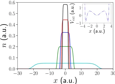
FIG. 1. The exact many-body electron density (solid lines) for a selection of the two-electron slab systems. The density is locally homogeneous across a plateau region and decays exponentially at the edges. Inset: the external potential for a typical two-electron slab system (middle density in main figure).

II. SET OF LDAS

A. LDAs from finite systems

In Ref. [27] we chose a set of finite locally homogeneous systems in order to mimic the HEG, which we referred to as “slabs” (Fig.1). We generated sets of one-electron (1e), two-electron (2e), and three-electron (3e) slab systems over a typical density range (up to 0.6 a.u.) and in each case calculated the exact xc energy Exc. From this we parametrized the xc energy densityεxc=Exc/N in terms of the electron density of the plateau region of the slabs, repeating for the 1e, 2e, and 3eset.

To approximate the xc energy of an inhomogeneous system, the LDA focuses on the local electron density at each point in the system:

E_xcLDA[n]=

n(x)εxc(n)dx, (1)

where in a conventional LDAεxc(n) is the xc energy density of a HEG of densityn. This approximation becomes exact in the limit of the HEG, and so it is a reasonable requirement for the finite LDAs to become exact in the limit of the slab systems. Due to the initial parametrization ofεxc(n) focusing on the plateau regions of the slabs (i.e., ignoring the inhomogeneous regions at the edges), we used arefinement process [27] in order to fulfill this requirement.

The refined form for the xc energy density in the three finite LDAs has now been increased from the four-parameter fit in Ref. [27] to a seven-parameter fit5in this paper:

εxc(n)=(A+Bn+Cn2+Dn3+En4+F n5)nG, (2)

5_{We have significantly increased the precision of the calculations}

for the slab systems in order to do this. The numerical difference between the new seven-parameter fits and original four-parameter fits is less than 1% inεxcacross the density range used in constructing the LDAs (except in the very low-density regionn <0.06 a.u.). This has allowed us to resolve the differences between the four LDAs in fine detail.

TABLE I. Optimal fit parameters forεxc(n) in the finite LDAs. The last two rows contain the mean absolute error (MAE) and root-mean-square error (RMSE) of the fits.εxc(n) is graphed in Sec.II D below.

Parameter 1evalue 2evalue 3evalue

A −1.2202 −1.0831 −1.1002

B 3.6838 2.7609 2.9750

C −11.254 −7.1577 −8.1618

D 23.169 12.713 15.169

E −26.299 −12.755 −15.776

F 12.282 5.3817 6.8494

G 7.4876×10−1 _7.0955×10−1 _7.0907×10−1

MAE 1.3×10−4 _1.2×10−4 _9.9×10−5

RMSE 1.9×10−3 _5.1×10−4 _3.8×10−4

where the optimal parameters for each LDA are given in Table I. The xc potential Vxc is defined as the functional derivative of the xc energy which in the LDA reduces to a simple form (see Supplemental Material [31])

V_xcLDA(n)=εxc(n(x))+n(x)

dεxc

dn

n(x)

. (3)

B. HEG exchange functional

In Ref. [27] we solved the Hartree-Fock equations to find the exact exchange energy densityεxfor a fully spin-polarized [ζ =1 where ζ ≡(N↑_−N↓_{)/N] 1D HEG of density n}

consisting of an infinite number of electrons interacting via the softened Coulomb repulsionu(x−x′)=(|x−x′| +1)−1:

εx(n)= − 1 8π2_n

π n

−π n

dk

π n

−π n

dk′u(k′−k), (4)

where the Fourier transform ofu(x−x′) is integrated over the plane defined by the Fermi wave vectorkF=π n.

Solving Eq. (4) for the range of densities we used in the finite LDAs, we parametrized εx(n). Once again, we have increased our fit from four parameters to seven parameters, as in Eq. (2) above (see Supplemental Material [31]). The optimal parameters are given in TableII. Theεx(n) curve is shown in the inset of Fig.2.

TABLE II. Optimal fit parameters forεx(n) in the HEG LDA. The last two rows contain the mean absolute error (MAE) and root-mean-square error (RMSE) of the fit.

Parameter Value

A −1.1511

B 3.3440

C −9.7079

D 19.088

E −20.896

F 9.4861

G 7.3586×10−1

MAE 6.5×10−5

RMSE 7.2×10−4

0.0 0.2 0.4 0.6

n

(a.u.)

−0.008 −0.006 −0.004 −0.002 0.000

ε

(a

.u

.)

fit LRDMC

0_.0 0_.2 0_.4 0_.6

n(a.u.)

−0.3 −0.2 −0.1 0.0

εx

(a

.u

.)

FIG. 2. Theεc(with associated error bars) for a set of HEGs over the density range used in the finite LDAs. The fit applied (solid blue) becomes exact in the known high- and low-density limits. Inset: the

εxcurve in the HEG LDA.

C. HEG correlation functional

We use the lattice regularized diffusion Monte Carlo (LRDMC) algorithm [28] to compute the ground-state energy of the fully spin-polarized HEG over a wide range of densities, much higher than the 0.6 a.u. limit used in the finite LDAs. This is in order to ensure the resultant parametrization of the correlation energy densityεcreduces to the known high- and low-density limits. We determineεcby subtracting the kinetic energy andεxcontributions from the total energy.

To parametrize the correlation energy density we use a fit of the form (see Supplemental Material [31])

εc(rs)= −

ARPArs+Ers2 1+Brs+Crs2+Drs3

ln(1+αrs+βrs2)

α , (5)

wherersis the Wigner-Seitz radius and is related to the density (in 1D) by 2rs=1/n. The optimal parameters (with estimated errors) are given in TableIII. The fit applied to the data is shown in Fig.2.

The high-density limit (infinitely weak correlation) of the parametrization is

εc(rs→0)= −ARPArs2, (6)

and its low-density limit (infinitely strong correlation) is

εc(rs→ ∞)= − 2E αD

ln(rs)

rs

. (7)

Therefore, the parametric form in Eq. (5) correctly reproduces the expected behavior of the correlation energy density in the high-density limit [32,33] [εc∝rs2] and low-density limit [εc∝ln(rs)/rs].

D. Comparison of 1e, 2e, 3e, and HEG LDAs

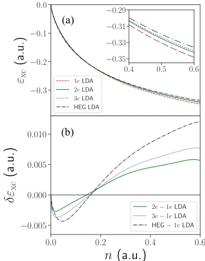
Summing together the HEG exchange and correlation parametric fits, we can now compare the HEG LDA that we have developed against the three finite LDAs. The striking similarity between the fourεxccurves can be seen in Fig.3(a). While very similar in the low-density range, there are some differences between them. These are highlighted in Fig.3(b) which, using the 1eLDA as a reference, plots its difference with

TABLE III. Optimal fit parameters with estimated errors in parentheses forεc(rs) in the HEG LDA. The last two rows contain the mean absolute error (MAE) and root-mean-square error (RMSE) of the fit. Note:ARPAhas been determined from the high-density limit for

εc(in which the random phase approximation (RPA) is exact [32,33]), which is exactly fulfilled by our fit, and hence has no associated error.

Parameter Value

ARPA 9.415195×10−4

B 2.601(5)×10−1

C 6.404(7)×10−2

D 2.48(3)×10−4

E 2.61(3)×10−6

α 1.254(2)

β 28.8(1)

MAE 2.4×10−5

RMSE 1.3×10−4

the remaining LDAs. There is a competing balance between exchange and correlation. At low densities, these differences can be mainly attributed toεc, which is entirely absent in the 1eLDA, and increases in magnitude as we progress to 2eto 3e

to HEG (Fig.4). As we move to higher densities in which the magnitude ofεcdecreases, and the magnitude ofεxincreases, the order of the four εxc curves reverses. They increasingly separate as we move to higher densities with the 1e LDA, which consists entirely of self-interaction correction, giving the

−0.3 −0.2 −0.1 0.0

ε

c

(a

.u

.)

1eLDA

2eLDA

3eLDA

HEG LDA

0.0 0.2 0.4 0.6

n

(a.u.)

−0.005

0_.000 0.005 0_.010

δ

ε

c

(a

.u

.)

2e−1eLDA

3e−1eLDA

HEG₋1eLDA

0_.4 0_.5 0_.6 −0.35

−0.33 −0.31 −0.29

0.4 0.5 0.6

−0.35

−0.33

−0.31

−0.29

0.4 0.5 0.6 −0.35

−0.33 −0.31 −0.29

FIG. 3. (a) Theεxc curves in the 1e(dashed red line), 2e(solid green line), 3e (dotted blue line), and HEG (dotted-dashed black line) LDAs. Inset: closeup of the four curves at higher densities. The similarity between them is striking, with a clear progression from 1e

M. T. ENTWISTLE, M. CASULA, AND R. W. GODBY PHYSICAL REVIEW B97, 235143 (2018)

0_.0 0_.2 0_.4 0_.6

n

(a.u.)

−0.006 −0.004 −0.002 0_.000

ε

(a

.u

.)

2eLDA

3eLDA HEG LDA

FIG. 4. We calculate the exactεcfor the 2e(solid green line) and 3e(dotted blue line) slab systems through Hartree-Fock calculations. We plot these against theεccurve in the HEG LDA (dotted-dashed black line). Theεcin the HEG LDA is much larger (∼2–3 that of the 3e LDA and∼3–4 that of the 2eLDA). While not a perfect comparison due to the refinement process used in the construction of the finite LDAs, it gives a useful indication of the size ofεcin theirεxccurves.

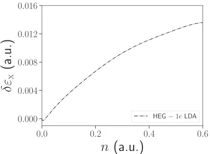
largest magnitude forεxc. By plotting the difference between the 1e LDA (where correlation is absent) and the exchange part of the HEG LDA (i.e., removing the correlation term), it can be seen that the 1eLDA yields a larger exchange energy density than the HEG LDA at all densities (Fig.5).

The refinement process used in the construction of the finite LDAs focused on giving the correct Exc in the limit of the slab systems, but did not ensure that the correctVxc, and by extension electron density, were reproduced (a property of HEG LDAs). We find that the finite LDAs are completely inadequate at reproducing the densities of the slab systems. We compare theexactVxcagainst nand find that there is a high nonlocal dependence onn, implying thatnolocal density functional can accurately reproduceVxcand hence nfor the slab systems. In light of this, the success of the finite LDAs reported below is all the more surprising.

0.0 0.2 0.4 0.6

n

(a.u.)

0_.000 0.004 0_.008 0.012 0_.016

δ

ε

(a

.u

.)

HEG −1eLDA

FIG. 5. The εx curve in the 1e LDA (εx=εxc) is used as a reference here. Plotted is its difference (δεx=εx−εx1e) with theεx curve in the HEG LDA (εx=εxc−εc). It can be seen that the 1e LDA yields a larger exchange energy density than the HEG LDA at all densities. Note: This is not true in the very low-density region (n <0.012), which we attribute to errors in the fits.

III. TESTING THE LDAs

In the previous section we observed the close similarity between the four LDAs. In this section we apply them to a range of model systems (see Supplemental Material [31]) in order to identify the differences between them.

A. Weakly correlated systems

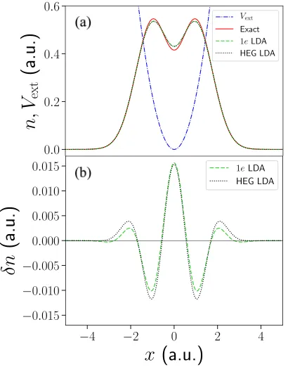
System 1 (2e harmonic well). We first consider a pair of interacting electrons in a strongly confining harmonic potential well (ω= 2₃a.u.) where correlation is very weak.6_We calculate the exact many-body electron density using iDEA, and compare it against the densities obtained from applying the LDAs self-consistently. There is a progression from the 1e–2e–3e–HEG LDA and so we choose to plot the 1eand HEG LDA densities (i.e., the 2e and 3e LDA densities lie between these) against the exact [Fig.6(a)]. Both LDAs match the exact density well, and so we plot their absolute errors (δn=nLDA−nexact) to more clearly identify their differences [Fig.6(b)]. The 1eLDA has a slightly smaller net absolute error (

|δn|dx). While the HEG LDA gives a slightly better electron density in the central region (dip in the density), the 1e

LDA better matches the decay of the density towards the edges of the system, and perhaps more interestingly, the two peaks in the density where the self-interaction correction is largest.

Due to the importance of energies in DFT calculations, we also compare the exact Exc and total energy Etotal, with those obtained from applying the LDAs self-consistently (TableIV). While all the LDAs give good approximations to both quantities, there are some significant differences due to this system being dominated by regions of high density, and theεxccurves separating in this limit (see Fig.3). As with the approximations to the electron density, there is a progression from the 1e–2e–3e–HEG LDA, with the 1eLDA reducing the absolute errors (δExc

Exc,

δE

E) in the HEG LDA by a factor of 5–6.

System 2 (3e harmonic well). Next, we consider a harmonic potential well with three electrons, but slightly less confining (ω=1₂), in order to avoid an unphysically high electron density (n >0.6 a.u.). As in the 2eharmonic well system, we find a progression from the 1e–2e–3e–HEG LDA, with all LDAs giving good electron densities [see Fig.7(a)for the 1eand HEG LDA densities plotted against the exact]. Again, the 1eLDA has the smallest net absolute error, and outperforms the rest of the LDAs in the regions where the density peaks [Fig.7(b)].

We also compare the exactExcandEtotalagainst the LDAs (TableIV). All LDAs give good energies, with some noticeable differences between them due to this system being dominated by regions of high density, like in the 2eharmonic well system. However, themagnitudeofExcin the 1eLDA is greater than the exact (i.e., it overestimates the amount of exchange +

correlation), and subsequently it gives a total energy lower than the exact. While the absolute error inExcfor each LDA is similar to that inEtotal, this overestimation of exchange+

6_{We calculate the absolute error between the exact electron}

den-sity and the denden-sity obtained from a self-consistent Hartree-Fock calculation (δn=nHF_−nexact_{), and find the net absolute error to} be

|δn|dx≈1.4×10−3_{. The correlation energy is 0.13% of the} exchange-correlation energy−0.62 a.u.

0.0

0_.2

0_.4

0_.6

n

,V

e

x

t

(a

.u

.)

Vext

Exact

1eLDA HEG LDA

−4 −2 0 2 4

x

(a.u.)

−0.015 −0.010 −0.005 0_.000 0.005 0_.010 0.015

δ

n

(a

.u

.)

1eLDA HEG LDA

FIG. 6. System 1 (two electrons in a harmonic potential well). (a) The external potential (dotted-dashed blue line), together with the exact electron density (solid red line), and the densities obtained from applying the 1e(dashed green line) and HEG (dotted black line) LDAs. Both LDAs are in very good agreement with the exact result. (b) The absolute error in the density (δn=nLDA_−nexact_{) in the 1e} (dashed green line) and HEG (dotted black line) LDAs, allowing their differences to be more clearly identified.

correlation in the 1eLDA results in the 2eLDA giving the best total energy.

B. A system dominated by the self-interaction correction

The self-interaction correction (SIC) isabsentin xc func-tionals constructed from the HEG. However, the xc energy of the 1eslab systems (which were used to construct the 1e

LDA) consists entirely of SIC. In the first two model systems, we found that the 1eLDA (and indeed the other finite LDAs) better describes the electron density in regions where the SIC is strongest, than the HEG LDA. We now investigate this further.

System 3 (2e double well). We choose a system with two electrons confined to a double-well potential. The wells are separated, such that the electrons arehighly localizedand can be considered as two separate subsystems [Fig. 8(a)]. This

0_.0 0_.2 0.4 0.6

n

,V

e

x

t

(a

.u

.)

Vext

Exact

1eLDA HEG LDA

−8 −4 0 4 8

x

(a.u.)

−0.015 −0.010 −0.005 0.000 0_.005 0.010 0.015

δ

n

(a

.u

.)

1eLDA HEG LDA

FIG. 7. System 2 (three electrons in a harmonic potential well). (a) The external potential (dotted-dashed blue line), together with the exact electron density (solid red line), and the densities obtained from applying the 1e(dashed green line) and HEG (dotted black line) LDAs. Much like the 2eharmonic well system, both LDAs match the exact density well. (b) The absolute error in the density in the 1e

(dashed green line) and HEG (dotted black line) LDAs. Again, the 1eLDA outperforms the HEG LDA in the density peaks, which is dominated by the self-interaction correction.

results in the Hartree potential being small outside of the wells, and being dominated by the electron self-interaction within the wells. Consequently, a large proportion of the xc potential is self-interaction correction. Applying the LDAs, we find the usual progression 1e–2e–3e–HEG. Focusing on the peaks in the electron density, the 1e LDA substantially reduces the error present in the HEG LDA [Fig.8(b)]. To understand this, we analyze the xc potential [Fig.8(c)]. The 1e LDA better reproduces the large dips inVxc, corresponding to the peaks in the electron density. Hence, the SIC is more effectively captured.

While the LDA errors in Exc are larger than in the first two systems, they are still small (4.8%–6.8%) (TableIV). The absolute errors inEtotalare similar.

TABLE IV. Total energies and xc energies for the set of weakly correlated systems (1–3), from exact calculations and from applying the four LDAs self-consistently (δELDA_=ELDA_−Eexact_{). Estimated errors are±1 in the last decimal place, unless otherwise stated in parentheses.}

System Etotal(a.u.) Exc(a.u.)

Exact δE1e

total δEtotal2e δEtotal3e δEHEGtotal Exact δExc1e δE2xce δE3xce δExcHEG

2eharmonic well 1.6932 0.0037 0.0126 0.0153 0.0211 −0.6192 0.0045 0.0137 0.0165 0.0225

3eharmonic well 3.1875 −0.0073 0.0065 0.0108 0.0199 −0.9305(5) −0.0058(5) 0.0085(5) 0.0129(5) 0.0223(5)

M. T. ENTWISTLE, M. CASULA, AND R. W. GODBY PHYSICAL REVIEW B97, 235143 (2018)

−0.8 −0.4 0.0 0.4

n

,V

e

x

t

(a

.u

.)

Vext

Exact

1eLDA HEG LDA

−0.012 −0.008 −0.004

0.000

0.004

0.008

δ

n

(a

.u

.)

1eLDA HEG LDA

−15 −10 −5 0 5 10 15

x

(a.u.)

−0.5 −0.4 −0.3 −0.2 −0.1

0.0

V

c

(a

.u

.)

Exact

1eLDA HEG LDA

FIG. 8. System 3 (two electrons in a double-well potential). (a) The external potential (dotted-dashed blue line), together with the exact electron density (solid red line), and the densities obtained from applying the 1e(dashed green line) and HEG (dotted black) LDAs. The wells are separated, such that the electrons are highly localized. (b) The absolute error in the density in the 1e(dashed green line) and HEG (dotted black line) LDAs. The 1eLDA is far superior in the regions where the density peaks, and hence where the Hartree potential is large and dominated by the electron self-interaction. (c) The exact xc potential (solid red line), and the xc potentials given by the 1e(dashed green line) and HEG (dotted line) LDAs. The dips in

Vxcare more closely matched by the 1eLDA due to it better capturing the self-interaction correction, present in the exactVxc.

C. Systems where correlation is stronger

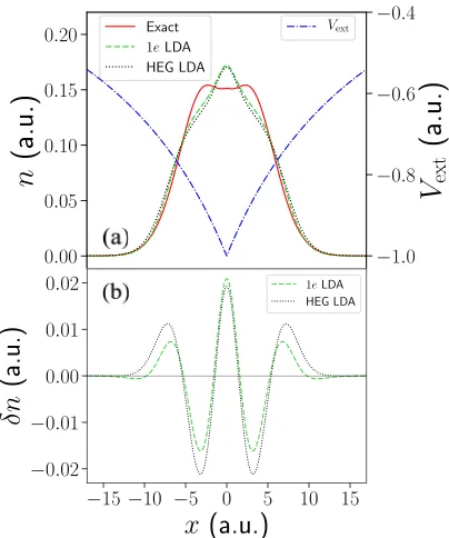
System 4 (2e atom). We now consider a system where the relative size of electron correlation increases significantly:7 two electrons confined to asoftenedatomiclike potentialVext=

−(|ax| +1)−1_{, where a =} 1

20. Although we find the same

7_{We calculate the absolute error between the exact electron}

den-sity and the denden-sity obtained from a self-consistent Hartree-Fock calculation (δn=nHF_−nexact_{), and find the net absolute error to} be

|δn|dx≈7.4×10−2_{. The correlation energy is 1.1% of the} exchange-correlation energy−0.37 a.u.

0.00 0_.05 0.10 0_.15 0_.20

n

(a

.u

.)

Exact

1eLDA HEG LDA

−1.0 −0.8 −0.6 −0.4

V

x

t

(a

.u

.)

Vext

−15−10 −5 0 5 10 15

x

(a.u.)

−0.02 −0.01 0_.00 0.01 0.02

δ

n

(a

.u

.)

1eLDA

HEG LDA

FIG. 9. System 4 (two electrons in a softened atomiclike poten-tial). (a) The external potential (dotted-dashed blue line), together with the exact electron density (solid red line), and the densities obtained from applying the 1e (dashed green line) and HEG (dotted black line) LDAs. Unlike in the weakly correlated systems, the LDAs give poor electron densities. (b) The absolute error in the density in the 1e

(dashed green line) and HEG (dotted black line) LDAs. While the net absolute errors are much larger than in the weakly correlated systems, the 1eLDA still performs the best.

progression (1e–2e–3e–HEG) as seen in the first three model systems, in which correlation was weak, all LDAs give in-adequate electron densities. This can be seen by plotting the 1eand HEG LDA densities against the exact [Fig.9(a)]. The LDAs give densities that are not even qualitatively correct, e.g., predicting a single peak in the center of the system, which is absent in the exact density. The net absolute errors are much larger than in the weakly correlated systems, however, the 1e

LDA once again gives the smallest [Fig.9(b)].

We find that although the LDA densities are poor, the xc energies are surprisingly good (TableV). This can be attributed somewhat(see Sec.III Dfor investigation of further causes) to errors in the density being partially canceled by errors inherent in the approximate xc energy functional [34]. We infer this by noting the progression (HEG–3e–2e–1e) when we apply the LDAs to the exactdensity, in contrast to the self-consistent solutions in TableV. As in the weakly correlated systems, the absolute errors inEtotalare smaller than inExc, due to a partial cancellation of errors from the Hartree energy component. It is much more apparent in this system due to the LDAs incorrectly predicting a central peak in the electron density [Fig.9(a)].

System 5 (3e atom). Finally, we consider three electrons in an external potential of the same form as the 2eatom, but less confining, witha =₅₀1. Along with the usual progression (1e–2e–3e–HEG), we find a similar result to the 2e atom, with the LDAs giving poor electron densities [Fig. 10(a)]. Although the densities are qualitatively correct, unlike in the

TABLE V. Total energies and xc energies for the set of strongly correlated systems (4 and 5), from exact calculations and from applying the four LDAs self-consistently (δELDA_=ELDA_−Eexact_{). Estimated errors are±1 in the last decimal place, unless otherwise stated in parentheses.}

System Etotal(a.u.) Exc(a.u.)

Exact δE1e

total δE2totale δE3totale δEtotalHEG Exact δExc1e δE2xce δExc3e δExcHEG

2eatom −1.5099 0.0053 0.0044 0.0032 0.0022 −0.3728 0.0084 0.0101 0.0099 0.0111

3eatom −2.3282(5) 0.0121(5) 0.0085(5) 0.0057(5) 0.0029(5) −0.493(4) 0.029(4) 0.029(4) 0.027(4) 0.028(4)

2e atom, the LDAs significantly underestimate the peaks in the electron density. Subsequently, the absolute errors are very large [Fig.10(b)]. The 1eLDA, along with giving the lowest net absolute error, most accurately reproduces the peaks in the density, where the SIC is largest.

While the absolute errors inExc are larger than in the 2e atom, they are still small (TableV). Again, this partially arises from applying approximate xc energy functionals to incorrect densities. As in the 2eatom, the absolute errors inEtotalare much lower than those inExc, due to a partial cancellation of errors from the Hartree energy component.

D. Cancellation of errors between exchange and correlation

HEG-based LDAs have been known to typically under-estimate the magnitude of the exchange energy Ex, while overestimating the magnitude of the correlation energyEc. Consequently, while the totalExcis underestimated in magni-tude, the approximation proves to be better than was originally expected due to a partial cancellation of errors.

0_.00 0.05 0_.10 0.15 0.20

n

(a

.u

.)

Exact

1eLDA HEG LDA

−1.0 −0.8 −0.6

V

x

t

(a

.u

.)

Vext

−30 −20 −10 0 10 20 30

x

(a.u.)

−0.03 −0.02 −0.01 0.00 0.01 0.02 0.03

δ

n

(a

.u

.)

1eLDA

HEG LDA

FIG. 10. System 5 (three electrons in a softened atomiclike poten-tial). (a) The external potential (dotted-dashed blue line), together with the exact electron density (solid red line), and the densities obtained from applying the 1e(dashed green line) and HEG (dotted black line) LDAs. Like in the 2eatom, the LDAs give poor electron densities. The 1eLDA more accurately reproduces the peaks in the density, where the SIC is largest. (b) The absolute error in the density in the 1e(dashed green line) and HEG (dotted black line) LDAs. Again, the net absolute errors are large, with the 1eLDA giving the smallest.

We investigate how well our HEG LDA approximatesEx and Ec in the model systems, and how this contributes to accurate values forExc. To do this we perform Hartree-Fock calculations for each of the model systems, and together with the exact solutions obtained through iDEA, are able to divide the exactExcinto its exchange and correlation components. We then apply the HEG LDA, which is split into separateEx andEcfunctionals, for comparison (TableVI). In all systems, the HEG LDA underestimates the magnitude of Ex, while it overestimates the magnitude of Ec. However, due to the exchange energy being the dominant component ofExc, even in strongly correlated systems, this only leads to a partial cancellation of errors.

The 1eLDA yields a larger magnitude forεxthan the HEG LDA across the entire density range studied (up to 0.6 a.u.) (Fig. 5), which arises from a better description of the SIC (Sec.III B). In the 1eLDA correlation is absent. Consequently, the 1exc energies that follow from TablesIVandVcan be considered as approximations toEx. We note that the 1eLDA substantially reduces the error inEx that arises in the HEG LDA.8_{We infer that this error reduction will also extend to the} 2eand 3eLDAs.

8_{This is also true in the 2edouble-well system where correlation is}

negligible, and the exchange energy is dominated by the SIC.

TABLE VI. Exchange energies and correlation energies for all systems (1–5), from exact calculations and from applying the HEG LDA self-consistently (δELDA_=ELDA_−Eexact_{). Estimated} errors are±1 in the last decimal place, unless otherwise stated in parentheses.

System Ex(a.u.)

Exact δEHEG

x

2eharmonic well −0.6184 0.0268

3eharmonic well −0.9286(5) 0.0276(5)

2edouble well −0.5349 0.0441

2eatom −0.3686 0.0185

3eatom −0.488(3) 0.041(3)

System Ec(a.u.)

Exact δEHEG

c

2eharmonic well −0.0008 −0.0043

3eharmonic well −0.0019 −0.0053

2edouble well −0.0000 −0.0077

2eatom −0.0042 −0.0074

M. T. ENTWISTLE, M. CASULA, AND R. W. GODBY PHYSICAL REVIEW B97, 235143 (2018)

IV. CONCLUSIONS

We have constructed an LDA based on the homogeneous electron gas (HEG) through suitable quantum Monte Carlo techniques and find that it is remarkably similar in many regards to a set of three LDAs constructed from finite systems. Applying them to test systems to explore the differences between them, we find that the finite LDAs give better densities and energies in highly confined systems in which correlation is weak. Most interestingly, the LDA constructed from systems of just one electron most accurately describes the self-interaction correction. All LDAs give poor densities in systems where correlation is stronger, but give reasonably good energies, with the HEG LDA giving the best total energies. Across all test systems, the HEG LDA underestimates the magnitude of the exchange energy and overestimates the magnitude of the correlation energy, leading to a partial cancellation of errors.

As a consequence of the finite LDAs giving a better description of the self-interaction correction, we infer that they would reduce the error in the exchange energy. Furthermore, we expect that finite LDA functionals will also provide a better treatment of the SIC for spinful electrons. Their derivation and usage could lead to an improved description of the electronic structure in a variety of situations, such as at the onset of Wigner oscillations.

Data created during this research is available by request from the York Research Database [35].

ACKNOWLEDGMENTS

M.C. acknowledges the GENCI allocation for computer resources under Project No. 0906493. We thank L. Talirz for recent developments in the iDEA code, and M. Hodgson and J. Wetherell for helpful discussions.

[1] P. Hohenberg and W. Kohn,Phys. Rev.136,B864(1964). [2] R. Dreizler and E. Gross,Density Functional Theory: An

Ap-proach to the Quantum Many-Body Problem(Springer, Berlin, 2012).

[3] R. Parr and W. Yang,Density-Functional Theory of Atoms and Molecules, International Series of Monographs on Chemistry (Oxford University Press, New York, 1994).

[4] C. Fiolhais, F. Nogueira, and M. Marques,A Primer in Density Functional Theory, Lecture Notes in Physics (Springer, Berlin, 2003).

[5] K. Burke,J. Chem. Phys.136,150901(2012).

[6] R. M. Martin,Electronic Structure: Basic Theory and Practical Methods(Cambridge University Press, Cambridge, 2004). [7] E. Engel and R. Dreizler, Density Functional Theory: An

Advanced Course, Theoretical and Mathematical Physics (Springer, Berlin, 2011).

[8] W. Kohn and L. J. Sham,Phys. Rev.140,A1133(1965). [9] D. M. Ceperley and B. J. Alder, Phys. Rev. Lett. 45, 566

(1980).

[10] G. Onida, L. Reining, and A. Rubio,Rev. Mod. Phys.74,601

(2002).

[11] M. Lein, E. K. U. Gross, and J. P. Perdew,Phys. Rev. B61,

13431(2000).

[12] O. Gritsenko, S. Van Gisbergen, A. Görling, E. Baerends,et al.,

J. Chem. Phys.113,8478(2000).

[13] N. T. Maitra, K. Burke, and C. Woodward,Phys. Rev. Lett.89,

023002(2002).

[14] K. Burke, J. Werschnik, and E. Gross, J. Chem. Phys. 123,

062206(2005).

[15] D. Varsano, A. Marini, and A. Rubio, Phys. Rev. Lett.101,

133002(2008).

[16] R. O. Jones and O. Gunnarsson,Rev. Mod. Phys.61,689(1989). [17] W. E. Pickett,Comput. Phys. Rep.9,115(1989).

[18] X. Gonze, P. Ghosez, and R. W. Godby,Phys. Rev. Lett.78,294

(1997).

[19] J. P. Perdew and A. Zunger,Phys. Rev. B23,5048(1981). [20] D. J. Tozer and N. C. Handy,J. Chem. Phys.109,10180(1998). [21] A. Dreuw, J. L. Weisman, and M. Head-Gordon,J. Chem. Phys.

119,2943(2003).

[22] M. Levy, J. P. Perdew, and V. Sahni, Phys. Rev. A30,2745

(1984).

[23] C.-O. Almbladh and U. von Barth,Phys. Rev. B31,3231(1985). [24] P. Mori-Sanchez and A. J. Cohen,Phys. Chem. Chem. Phys.16,

14378(2014).

[25] M. A. Mosquera and A. Wasserman,Phys. Rev. A89,052506

(2014).

[26] M. A. Mosquera and A. Wasserman, Mol. Phys. 112, 2997

(2014).

[27] M. T. Entwistle, M. J. P. Hodgson, J. Wetherell, B. Longstaff, J. D. Ramsden, and R. W. Godby,Phys. Rev. B94,205134(2016). [28] M. Casula, C. Filippi, and S. Sorella,Phys. Rev. Lett.95,100201

(2005).

[29] M. J. P. Hodgson, J. D. Ramsden, J. B. J. Chapman, P. Lillystone, and R. W. Godby,Phys. Rev. B88,241102(2013).

[30] A. Gordon, R. Santra, and F. X. Kärtner,Phys. Rev. A72,063411

(2005).

[31] See Supplemental Material athttp://link.aps.org/supplemental/ 10.1103/PhysRevB.97.235143 for the parametric form of the xc potential in the finite LDAs, for the parametric form of the exchange potential in the HEG LDA, for the parameters of the model systems, and details on our calculations to obtain converged results.

[32] M. Casula, S. Sorella, and G. Senatore,Phys. Rev. B74,245427

(2006).

[33] L. Shulenburger, M. Casula, G. Senatore, and R. M. Martin,J. Phys. A: Math. Theor.42,214021(2009).

[34] M.-C. Kim, E. Sim, and K. Burke,Phys. Rev. Lett.111,073003

(2013).

[35] M. T. Entwistle, M. Casula, and R. W. Godby, (2018), doi:

10.15124/65cd1dd8-c240-45a5-9a47-0ac6ff870f51.